Shot Noise of coupled Semiconductor Quantum Dots

Abstract

The low-frequency shot noise properties of two electrostatically coupled semiconductor quantum dot states which are connected to emitter/collector contacts are studied. A master equation approach is used to analyze the bias voltage dependence of the Fano factor as a measure of temporal correlations in tunneling current caused by Pauli’s exclusion principle and the Coulomb interaction. In particular, the influence of the Coulomb interaction on the shot noise behavior is discussed in detail and predictions for future experiments will be given. Furthermore, we propose a mechanism for negative differential conductance and investigate the related super-Poissonian shot noise.

I Introduction

Shot noise investigations in mesoscopic systems can reveal information of transport properties which are not accessible by conductance measurements alone Blanter and Büttiker (2000). In particular, the dynamic correlations in the tunneling current through double-barrier structures caused by Pauli’s exclusion principle can provide information regarding the barrier geometry Chen and Ting (1991). If the charging energy of bound states becomes larger than the thermal energy as in the case of small quantum dots (QDs), strong Coulomb correlations occur and have an additional influence on the shot noise. For metallic QDs the zero-frequency Fano factor which quantifies correlations with respect to the uncorrelated Poissonian noise Schottky (1918) was analyzed by a master equation approach including the Coulomb blockade effect in Ref. Hershfield et al. (1993). At the steps of the resulting Coulomb staircase the Fano factor shows dips caused by Coulomb correlations which is quantitatively confirmed in the experiment Birk et al. (1995). In Ref. Hanke et al. (1993) a similar theoretical approach was applied to determine the finite-frequency shot noise of metallic QDs.

Despite that, for semiconductor QDs a comprehensive picture of the bias dependent shot noise behavior and a subsequent comparison with experimental data is not available at the moment. Some theoretical work has been done: the investigation of the Fano factor of an ensemble of states with statistically varying positions in a barrier by a classical approach Nazarov and Struben (1996); analytical bias dependence of the Fano factor for zero-temperature with non-equilibrium Green’s functions Wei et al. (1999); bias dependence of spin-dependent coherent tunneling Souza et al. (2002); shot noise in the co-tunneling regime Sukhorukov et al. (2001); in the Kondo-regime Meir and Golub (2002). In Ref. Wang et al. (1998) a numerical investigation of a spatially extended QD by means of a coherent technique was presented. In the current plateau regime the authors find a suppressed Fano factor which is smaller than one half for symmetric barriers in contradiction to the result of Chen and Ting (1991). In contrast, an enhanced Fano factor at the current steps was found. All of the above references mainly consider the noise due to negative correlations (sub-Poissonian noise). In the case of negative differential conductance in the current-voltage characteristic, e.g. in resonant tunneling diodes, positive correlations lead to super-Poissonian noise Iannaccone et al. (1998). Furthermore, in capacitively coupled metallic QDs super-Poissonian noise can occur Gattobigio et al. (2002).

Recently, the measurement of the low-frequency shot noise of tunneling through an ensemble of self-organized QDs was presented in Ref. Nauen et al. (2002) which primarily motivates this work. The current-voltage characteristic for low bias is dominated by steps which are presumably due to tunneling through few QD ground states which are well separated in energy (see also Itskevich et al. (1996); Narihiro et al. (1997); Hapke-Wurst et al. (1999)). The corresponding Fano factor shows an average noise suppression on the current plateau which enables the determination of the effective collector barrier thickness, given the known thickness of the emitter barrier Nauen et al. (2002). At the current steps, Fano factor peaks appear which we have considered theoretically by a master equation approach Kießlich et al. (2002a). It was shown that for tunneling through QD states which are not subject to Coulomb interaction, Fano factor peaks at the bias position of current steps occur, caused by Pauli’s exclusion principle. Good qualitative agreement with experiment was found.

The goal of this paper is the exemplary demonstration of the influence of the Coulomb interaction upon the Fano factor in a system of two QD states, its interplay with Pauli’s exclusion principle, and the consequences for future noise experiments where Coulomb interaction is present. The outline of the paper is as follows: in Sec. II a brief description of the master equation formalism Beenakker (1991) and the calculation of spectral power density (where we mainly follow the lines of Ref. Hershfield et al. (1993)) is given. Sec. III contains the results of the bias dependent Fano factor for varying Coulomb interaction energy and in Sec. IV the super-Poissonian shot noise related to negative differential conductance will be discussed. All results will be summarized in Sec. V.

II Model

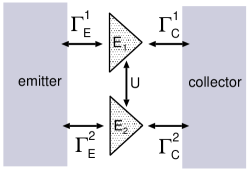
Figure 1: Scheme of the tunneling structure with rates $\Gamma_{E/C}^{i}$ ($i=1,2$) between two QDs and the emitter/collector, respectively; single-particle levels $E_{1/2}$, and Coulomb interaction energy $U$

The spectral power density of the current fluctuations is related to the autocorrelation function of the current by the Wiener-Khintchine theorem:

$$S_{ab}(\omega)=2\int_{-\infty}^{\infty}dte^{i\omega t}\left(\langle I_{a}(t)I_{b}(0)\rangle-\langle I\rangle^{2}\right)$$ (1)

where $a,b=E,C$ (emitter/collector) and $\langle\cdot\rangle$ denotes the ensemble average. A certain state $\nu=(n_{1},\dots,n_{N})$ (occupation numbers $n_{i}\in\{0,1\}$) at a time $t$ of the considered QD system with $N$ single-particle states is described by the respective occupation probability $P_{\nu}(t)$. The single-particle states may correspond to different energy levels in the same QD, or in different QDs. The time evolution of these occupation probabilities is determined by sequential tunneling of an electron into or out of the emitter/collector contact with the tunneling rates $\Gamma_{E/C}^{i}$ ($i$ labels the single-particle QD state) and can be written as a master equation in the general form

$$\dot{\mathbf{\underline{P}}}=\mathbf{\underline{\underline{M}}}\,\mathbf{\underline{P}}$$ (2)

Note that this approach holds only for weakly coupled QDs, $\Gamma_{E/C}^{i}\ll k_{B}T$, and cannot account for co-tunneling processes, i.e. coherent tunneling of two electrons simultanously Sukhorukov et al. (2001); Grabert and Devoret (1992). In this paper we consider two QD states $E_{1/2}$ in two different QDs which are connected to the emitter/collector contact and are coupled electrostatically by Coulomb interaction of strength $U$ (see Fig. 1). Then the vector of the occupation probabilities is $\mathbf{\underline{P}}=(P_{(0,0)},P_{(1,0)},P_{(0,1)},P_{(1,1)})^{T}$ and the transition matrix in (2) reads Beenakker (1991)

$$\mathbf{\underline{\underline{M}}}=\left(\begin{array}[]{cccc}-\Gamma_{E}^{1}f_{E}^{1}-\Gamma_{E}^{2}f_{E}^{2}&\Gamma_{E}^{1}(1-f_{E}^{1})+\Gamma_{C}^{1}&\Gamma_{E}^{2}(1-f_{E}^{2})+\Gamma_{C}^{2}&0\\ \Gamma_{E}^{1}f_{E}^{1}&-\Gamma_{E}^{1}(1-f_{E}^{1})-\Gamma_{C}^{1}-\Gamma_{E}^{2}f_{E}^{2,U}&0&\Gamma_{E}^{2}(1-f_{E}^{2,U})+\Gamma_{C}^{2}\\ \Gamma_{E}^{2}f_{E}^{2}&0&-\Gamma_{E}^{1}f_{E}^{1,U}-\Gamma_{E}^{2}(1-f_{E}^{2})-\Gamma_{C}^{2}&\Gamma_{E}^{1}(1-f_{E}^{1,U})+\Gamma_{C}^{1}\\ 0&\Gamma_{E}^{2}f_{E}^{2,U}&\Gamma_{E}^{1}f_{E}^{1,U}&\Gamma_{E}^{1}f_{E}^{1,U}+\Gamma_{E}^{2}f_{E}^{2,U}-\Gamma\end{array}\right)$$ (7)

with $\Gamma:=\Gamma_{C}^{1}+\Gamma_{C}^{2}+\Gamma_{E}^{1}+\Gamma_{E}^{2}$ and the Fermi functions in the emitter $f_{E}^{i}=(1+\exp{((E_{i}-e\eta V)/(k_{B}T))})^{-1}$ and $f_{E}^{i,U}=(1+\exp{((E_{i}+U-e\eta V)/(k_{B}T))})^{-1}$. $V$ is the bias voltage, $\eta V$ is the voltage drop across the emitter barrier, and $f_{E}^{i,U}$ includes the Coulomb interaction energy $U$ of the occupied QDs. For $eV\gg k_{B}T$ we neglect tunneling from the collector into the QDs, setting the collector occupation probability $f_{C}^{i}=f_{C}^{i,U}=0$.

The steady state solution of (2) can be obtained by

$$\mathbf{\underline{\underline{M}}}\,\mathbf{\underline{P}}^{0}=0$$ (8)

In order to calculate the current flowing through the system current operators are introduced. The current operators at the collector barrier with $f_{C}^{i}=f_{C}^{i,U}=0$ and at the emitter barrier, respectively, are defined by

$$\mathbf{\underline{\underline{j}}}_{C}=e\left(\begin{array}[]{cccc}0&\Gamma_{C}^{1}&\Gamma_{C}^{2}&0\\ 0&0&0&\Gamma_{C}^{2}\\ 0&0&0&\Gamma_{C}^{1}\\ 0&0&0&0\end{array}\right)$$ (13)

$$\mathbf{\underline{\underline{j}}}_{E}=e\left(\begin{array}[]{cccc}0&-\Gamma_{E}^{1}(1-f_{E}^{1})&-\Gamma_{E}^{2}(1-f_{E}^{2})&0\\ \Gamma_{E}^{2}f_{E}^{2}&0&0&-\Gamma_{E}^{1}(1-f_{E}^{1,U})\\ \Gamma_{E}^{1}f_{E}^{1}&0&0&-\Gamma_{E}^{2}(1-f_{E}^{2,U})\\ 0&\Gamma_{E}^{1}f_{E}^{1,U}&\Gamma_{E}^{2}f_{E}^{2,U}&0\end{array}\right)$$ (18)

so that the stationary mean current reads

$$\langle I\rangle=\sum_{\nu}[\mathbf{\underline{\underline{j}}}_{C}\mathbf{\underline{P}}^{0}]_{\nu}=\sum_{\nu}[\mathbf{\underline{\underline{j}}}_{E}\mathbf{\underline{P}}^{0}]_{\nu}$$ (19)

In the stationary limit the current at the collector barrier equals the mean current at the emitter barrier. For the calculation of the stationary current in (19) the current operators (13) could also be defined in diagonal form without changing the result (19). But for the determination of the current-current correlator (see below) the definition (13) becomes crucial as it projects the occupation probability to the state after an electron traversed the barrier.

To define the autocorrelation function of the current the time propagator $\mathbf{\underline{\underline{T}}}(t)$ is introduced as follows:

$$\mathbf{\underline{\underline{T}}}(t)\equiv\exp{(\mathbf{\underline{\underline{M}}}t)}\quad\textrm{with}\quad\mathbf{\underline{P}}(t)=\mathbf{\underline{\underline{T}}}(t)\,\mathbf{\underline{P}}(0)$$ (20)

With (8),(13), and (20) the current-current correlator in (1) is Hershfield et al. (1993)

$$\langle I_{a}(t)I_{b}(0)\rangle = \theta(t)\sum_{\nu}[\mathbf{\underline{\underline{j}}}_{a}\,\mathbf{\underline{\underline{T}}}(t)\,\mathbf{\underline{\underline{j}}}_{b}\mathbf{\underline{P}}^{0}]_{\nu}+$$ (21)

$$+\theta(-t)\sum_{\nu}[\mathbf{\underline{\underline{j}}}_{b}\,\mathbf{\underline{\underline{T}}}(-t)\,\mathbf{\underline{\underline{j}}}_{a}\mathbf{\underline{P}}^{0}]_{\nu}+$$

$$+e\delta_{ab}\delta(t)\sum_{\nu}\left|[\mathbf{\underline{\underline{j}}}_{a/b}\mathbf{\underline{P}}^{0}]_{\nu}\right|$$

($\theta(t)$ is the Heaviside function). The first two terms of the right-hand side in (21) contain the correlation between tunneling events at different times. The last term describes the self-correlation of a tunneling event at the same barrier (for further discussions of (21) see Davis et al. (1992); Hershfield et al. (1993); Korotkov (1994)).

For $\omega\ll\Gamma_{E/C}^{i}$ ($i=1,2$) which is the regime where experimental data are available at the moment (e.g. Nauen et al. (2002)), the spectral power densities become constant and $S_{EE}(0)=S_{CC}(0)=S_{EC}(0)=S_{CE}(0)\equiv S(0)$ holds.

As a measure of deviation from the uncorrelated Poissonian noise the dimensionless Fano factor $\alpha$ is used Blanter and Büttiker (2000):

$$\alpha(0) \equiv \frac{S(0)}{S_{P}}$$ (22)

$$\textrm{with}\quad S_{P} = 2e\langle I\rangle\quad\textrm{(Poissonian noise \cite[cite]{\@@bibref{Authors Phrase1YearPhrase2}{SCH18}{\@@citephrase{(}}{\@@citephrase{)}}})}$$

III Coulomb interacting quantum dots

We consider the tunneling through two non-degenerate QD ground states $E_{1}$ and $E_{2}$ with an energy separation $\Delta E=E_{2}-E_{1}$ which could correspond to slightly different QD sizes. The coupling to the emitter and collector contact will be assumed to be the same for both states: $\Gamma_{E}\equiv\Gamma_{E}^{1}=\Gamma_{E}^{2}$ and $\Gamma_{C}\equiv\Gamma_{C}^{1}=\Gamma_{C}^{2}$.

In the following we discuss three cases for the Coulomb interaction energy $U$: A. $U=0$, B. $U<\Delta E$, and C. $U>\Delta E$.

III.1 Noninteracting states: $U=0$

In Figs. 2 and 3 the results of a calculation for variation of $U$ in the range of a few $k_{B}T$ are shown (for fixed $k_{B}T=\Delta E$/23 and $\gamma=$5). The mean current $\langle I\rangle$ vs. bias voltage $V$ is plotted in Fig. 2a. For $U=0$ there are two steps due to tunneling through the respective states. The width of the current steps is determined by the Fermi distribution of the emitter electrons. Note that typical energy scales are as follows: the bias voltage $V$ is of the order of tens of mV, $\Delta E$ can be of the order of a few meV, $k_{B}T$ is of the order of tens of $\mu$eV for temperatures in the range of a few Kelvins.

The respective Fano factor $\alpha$ (22) is shown in Fig. 2b. On the first plateau in the current-voltage curve of Fig. 2a where only tunneling through one single-particle state occurs the Fano factor becomes

$$\alpha_{i}\equiv\alpha_{i}(0)=1-\frac{2}{\gamma_{i}+2+\frac{1}{\gamma_{i}}}f_{E}^{i}$$ (23)

$$\textrm{with}\quad\gamma_{i}\equiv\frac{\Gamma_{C}^{i}}{\Gamma_{E}^{i}}$$

where $i=1$ denotes the energetically lowest state. For $f_{E}^{1}=1$ eq. (23) is the well-known relation derived by L. Y. Chen et al. Chen and Ting (1991). It reflects the sensitivity of the Fano factor to Pauli’s exclusion principle. This is shown by the full curve $\alpha(\gamma)$ in Fig. 4: For symmetric tunneling barriers $\alpha$ is equal to one half and approaches unity for strong asymmetry. For bias voltages below the current onset where $f_{E}^{1}\approx 0$ the tunneling current becomes uncorrelated so that $\alpha_{1}=1$. At the second step where the second single-particle state is filled the Fano factor (Fig. 2b) has a peak which is also an effect of Pauli’s exclusion principle and we obtain a simple analytical expression for an arbitrary number of noninteracting QD states (for a derivation for two states see Appendix A):

$$\alpha=\frac{\sum_{i}\langle I_{i}\rangle\alpha_{i}}{\langle I\rangle}$$ (24)

by (23), where the current through state $i$ is: $\langle I_{i}\rangle=e\frac{\Gamma_{C}^{i}}{1+\gamma_{i}}f_{E}^{i}$, and the net current is $\langle I\rangle=\sum_{i}\langle I_{i}\rangle$. Eq. (24) was applied to the measured Fano factor modulation of tunneling through self-organized QDs Nauen et al. (2002) in a bias regime where only a few QD ground states are active in transport. It can qualitatively reproduce the measured Fano factor dependence upon the bias voltage Kießlich et al. (2002a).

III.2 $U<\Delta E$

With increasing Coulomb interaction $U\neq 0$ the Fano factor peak vanishes (see Fig. 2b) while the current changes only slightly. This underlines again the strong sensitivity of shot noise to correlations.

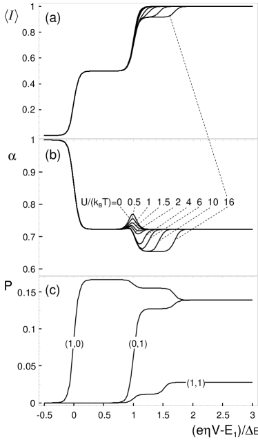
Figure 2: a) Normalized mean current $\langle I\rangle$ vs. bias voltage $V$. b) Fano factor $\alpha$ vs. bias voltage $V$ for different values of the Coulomb interaction energy $U$. c) Occupation probabilities $P_{(1,0)}$, $P_{(0,1)}$, and $P_{(1,1)}$ vs. bias voltage $V$ for $U/k_{B}T=$16. Parameters: $k_{B}T=\Delta E$/23, $\gamma=\Gamma_{C}/\Gamma_{E}=$5.

Further increase of $U$ leads to an additional step whose bias voltage is proportional to $U$. The respective occupation probabilities $P_{(1,0)}$, $P_{(0,1)}$, and $P_{(1,1)}$ for $U=16k_{B}T$ are shown in Fig. 2c: at the first plateau the electrons tunnel through the energetically lowest state $(1,0)$; the second plateau is generated by tunneling through both single-particle states with different probabilities and with lower probability through the two-particle state which is determined by the coupling to the collector. This correlated state originates from aligning the emitter Fermi energy with the energy $E_{1}+\Delta E$ of the second single-particle state which can be filled then. If the system is in the state $(0,1)$, a second electron may enter the $i=1$ level, as $U<\Delta E$. In contrast, the level $i=2$ is not accessible from the state $(1,0)$ as long as $\eta V<E_{1}+\Delta E+U$. This explains the asymmetry between the occupation probabilities $P_{(1,0)}$ and $P_{(0,1)}$. The height of this second plateau depends on the ratio of the tunneling rates: $\propto(1+\gamma)^{-1}$ with $\gamma:=\Gamma_{C}/\Gamma_{E}$.

At the second plateau in the current-voltage characteristic the Fano factor differs from the case of $U=0$, where only Pauli’s exclusion principle plays a role. The dependence on the ratio of tunneling rates $\gamma$ is shown by the dotted curve in Fig. 4. In contrast to the noninteracting regime the minimum is now at $\gamma=2$ with $\alpha=5/9$. These are numerical values, as we did not obtain an analytical expression for this Coulomb correlated state.

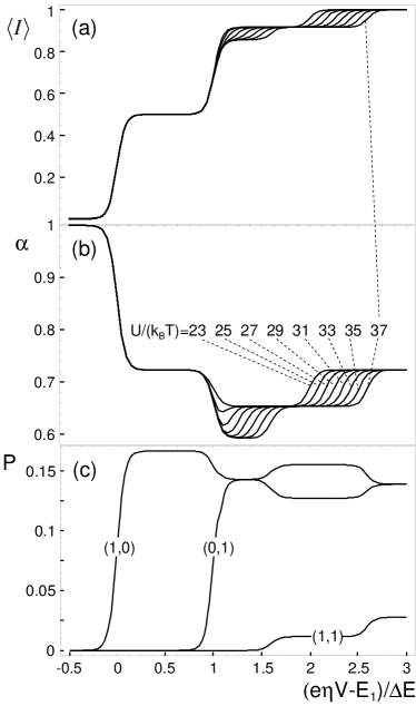
Figure 3: Same as Fig. 2, but for different values of $U$. c) $U/k_{B}T=$37.

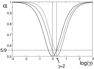
Figure 4: Fano factor $\alpha$ vs. ratio of tunneling rates $\gamma=\Gamma_{C}/\Gamma_{E}$. Full curve: first current plateau in Fig. 3; Dashed curve: second current plateau; Dotted curve: third current plateau. $U=37k_{B}T$.

In the experiment of Ref. Nauen et al. (2002) the question arises whether the QD states which are contributing to transport are Coulomb interacting. One way of determining this question would be the analysis of the Fano factor dependence upon the tunneling rate ratio $\gamma$ as shown in Fig. 4. However, in the experimental setup of Ref. Nauen et al. (2002) these rates are determined by the growth procedure. Therefore, they cannot be varied in the same sample. Here, we propose how to obtain the information about Coulomb correlations via the temperature dependence of the Fano factor. In Fig. 5 the Fano factor $\alpha$ vs. bias voltage $V$ for different temperatures $T$ in the bias range of the second current step of Fig. 2 is plotted. For noninteracting QD states (Fig. 5a) the Fano factor peak gets broader and experiences a slight shift to lower bias voltages for increasing temperatures. A qualitatively different picture results for interacting QD states in Fig. 5b ($U=\Delta E/46$): with increasing temperature the peak increases and also shifts to lower voltages. Hence, a unique fingerprint of Coulomb interaction of QD states even for very small $U$ shows up in the temperature dependence of the Fano factor peaks. Experimental investigations of this are in progress Nauen and Haug (2003).

Figure 5: Temperature dependence of the Fano factor vs. bias voltage $V$ for $\gamma=$5. a) $U=0$. b) $U=\Delta E$/46

III.3 $U>\Delta E$

For $U>\Delta E$ a fourth step arises in the current vs. bias voltage characteristic in Fig. 3a). Now, the second current plateau corresponds to a different state as in section B. Due to $U>\Delta E$ only the two single-particle states can be filled with the same probability (compare Fig. 3c). The respective Fano factor dependence upon $\gamma$ is (as discussed in Ref. Nazarov and Struben (1996))

$$\alpha=1-\frac{2\tilde{\Gamma}_{E}\Gamma_{C}}{(\tilde{\Gamma}_{E}+\Gamma_{C})^{2}}\quad\textrm{with}\quad\tilde{\Gamma}_{E}=2\Gamma_{E}$$ (25)

and is shown by the dashed curve in Fig. 4. The effect of Coulomb correlation upon the Fano factor consists substituting $\Gamma_{E}$ by $2\Gamma_{E}$ in eq. (23) and leads to a shift of the minimum of the full curve in Fig. 4 by $\gamma=2$. For $\gamma=$1 the Fano factor is $\alpha=$5/9.

IV Super-Poissonian noise

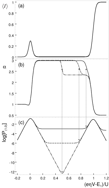
Figure 6: a) Normalized mean current $\langle I\rangle$ vs. bias voltage $V$. b) Fano factor $\alpha$ vs. bias voltage $V$. c) Occupation probability $P_{(1,0)}$ vs. bias voltage (logarithmic scale) for $\gamma_{2}=0$ (dash-dotted curve), $\gamma_{2}=10^{-6}$ (dashed curve), $\gamma_{2}=0.001$ (full curve). Parameters: $\gamma_{1}=1$, $k_{B}T=U$/23, $\Delta E=$0. Note that all three curves coincide in (a).

Figure 7: Fano factor $\alpha$ vs. $\gamma_{2}$ at $(e\eta V-E_{1})/U=$0.2 in Fig. 6b.

In the previous section we used identical rates $\Gamma_{C/E}$ for both states. Now, we allow their couplings to the collector contact to be different: $\Gamma_{C}^{1}\neq\Gamma_{C}^{2}$. For $\gamma_{2}\leq 0.45\gamma_{1}$ this leads to negative differential conductance (NDC) in the current-voltage characteristic as shown in Fig. 6a ($\Delta E=0$) Kießlich et al. (2002b). If the tunneling rate to the collector of state $i=2$ is much smaller than the other one the occupation probability $P_{(0,1)}$ becomes close to unity. The current carried by this state is proportional to $\Gamma_{C}^{2}$ and therefore low. Consequently, the occupation probability $P_{(1,0)}$ is low except close to the current onset where the respective current peak arises and around the bias voltage where the two-particle state $(1,1)$ becomes occupied. (compare Fig. 6c). Let us consider the dependence of the Fano factor on the bias voltage in Fig. 6b: in the bias voltage range where the current is suppressed the Fano factor is larger than unity (super-Poissonian shot noise caused by positive correlations of tunneling events). This is similar to the situation in a resonant tunneling diode Iannaccone et al. (1998). The Fano factor exhibits two different values separated by a step in the middle of the NDC-region (dashed curve in Figs. 6b) and c)) marked by arrows. The Fano factor dependence on $\gamma_{2}$ in the regime where $P_{(1,0)}$ decreases or keeps constant is shown in Fig. 7. This is the actual NDC regime: for $\gamma_{2}\rightarrow 0$ $\alpha$ approaches 3. In the bias regime where $P_{(1,0)}$ starts to increase due to thermally activated electrons (arrows in Fig. 6c) the Fano factor is lowered due to the effect of Pauli’s exclusion principle. Its value depends on the coupling ratio $\gamma_{1}$.

V Conclusions

We have investigated the low-frequency shot noise behavior in tunneling through two non-degenerate QD states which interact electrostatically. For noninteracting states the respective non-equilibrium current-voltage characteristic shows steps due to resonant tunneling through the single-particle states. In this case we have derived an explicit analytical expression for the bias dependence of the Fano factor. For interacting states additional current steps occur which are associated with Coulomb correlated states. The influence of the couplings to the collector upon the Fano factor has been clarified. We have developed sensitive tools to determine whether states are Coulomb correlated in tunneling experiments through self-organized QDs. This can be done by investigating the temperature dependence of the Fano factor vs. bias voltage at steps in the current-voltage characteristic.

Furthermore, we have examined an NDC mechanism in a system where the two states are coupled to the collector with different tunneling rates. Then the weakly coupled state blocks the other state by the Coulomb interaction. For degenerate states a current peak occurs and we have analyzed the Fano factor which becomes larger than unity (super-Poissonian noise due to positive correlations) in the bias range where the current is Coulomb blocked. In the limit of vanishing coupling of one state to the collector, we find $\alpha=$3.

Appendix A Analytical evaluation of the Fano factor for two noninteracting states

The stationary probability that level $i$ is occupied is $p_{i}\equiv\frac{\Gamma_{E}^{i}f_{E}^{i}}{\Gamma^{i}}$ or unoccupied $1-p_{i}$ ($\Gamma^{i}:=\Gamma_{E}^{i}+\Gamma_{C}^{i}$). Then the stationary occupation probability of the noninteracting two-level system given by (8) reads

$$\mathbf{\underline{P}^{0}}=\left(\begin{array}[]{c}(1-p_{1})(1-p_{2})\\ p_{1}(1-p_{2})\\ p_{2}(1-p_{1})\\ p_{1}p_{2}\end{array}\right)$$ (30)

since in the uncorrelated case the occupation probability for each state factorizes into the occupation probabilities of the single levels. By inserting this vector into (19) one immediately sees that terms with $p_{i}p_{j}$ cancel and the current is the sum of the currents through each level $i$: $\langle I_{i}\rangle=e\Gamma_{C}^{i}p_{i}$. This also holds for an arbitrary number of levels: $\langle I\rangle=\sum_{i}\langle I_{i}\rangle$.

Now, let us consider the time propagator (20): its matrix elements $T_{\nu\mu}(t)$ describe the conditional probability to have state $\nu$ at time $t$ under the condition of state $\mu$ at $t=0$. The matrix element $T_{\nu\mu}(t)\equiv T_{\mu\rightarrow\nu}(t)$ can be factorized for each level $i$ with the following conditional probabilities:

$$n_{i} = 0\rightarrow 1:\quad p_{i}(1-e^{-\Gamma^{i}t})$$

$$n_{i} = 1\rightarrow 0:\quad(1-p_{i})(1-e^{-\Gamma^{i}t})$$

$$n_{i} = 0\rightarrow 0:\quad 1-p_{i}(1-e^{-\Gamma^{i}t})$$

$$n_{i} = 1\rightarrow 1:\quad p_{i}+e^{-\Gamma^{i}t}(1-p_{i})$$ (31)

Due to the form of the current operator at the collector barrier in (13) the first row and last column of the matrix $\mathbf{\underline{\underline{T}}}(t)$ does not enter in the calculation of the current-current correlator (21). Carrying out the sum in (21) for two levels leads to

$$\langle I_{C}(t)I_{C}(0)\rangle= \ 2e\Gamma_{C}^{1}\left\{[\langle I_{1}\rangle p_{1}(1-p_{2})+\langle I_{2}\rangle p_{2}(1-p_{1})][T_{(0,0)\rightarrow(1,0)}+T_{(0,0)\rightarrow(1,1)}]\right.$$

$$\left.+\langle I_{2}\rangle p_{1}[T_{(1,0)\rightarrow(1,0)}+T_{(1,0)\rightarrow(1,1)}]+\langle I_{1}\rangle p_{2}[T_{(0,1)\rightarrow(1,0)}+T_{(0,1)\rightarrow(1,1)}]\right\}$$

$$+2e\Gamma_{C}^{2}\left\{[\langle I_{1}\rangle p_{1}(1-p_{2})+\langle I_{2}\rangle p_{2}(1-p_{1})][T_{(0,0)\rightarrow(0,1)}+T_{(0,0)\rightarrow(1,1)}]\right.$$

$$\left.+\langle I_{2}\rangle p_{1}[T_{(1,0)\rightarrow(0,1)}+T_{(1,0)\rightarrow(1,1)}]+\langle I_{1}\rangle p_{2}[T_{(0,1)\rightarrow(0,1)}+T_{(0,1)\rightarrow(1,1)}]\right\}$$

$$+e\langle I\rangle\delta(t)$$ (32)

Replacing the $T_{\mu\rightarrow\nu}$ in (32) by using the rules (31) the correlator becomes

$$\langle I_{C}(t)I_{C}(0)\rangle= \ -2\langle I_{1}\rangle^{2}e^{-\Gamma^{1}t}-2\langle I_{2}\rangle^{2}e^{-\Gamma^{2}t}+\langle I\rangle^{2}$$

$$+e\langle I\rangle\delta(t)$$ (33)

which can be generalized for an arbitrary number of levels

$$\langle I_{C}(t)I_{C}(0)\rangle= \ -2\sum_{i}\langle I_{i}\rangle^{2}e^{-\Gamma^{i}t}+\langle I\rangle^{2}$$

$$+e\langle I\rangle\delta(t)$$ (34)

The time-independent term in (33) and (34) cancels out in the calculation of the spectral power density (1) and we obtain

$$S(0)=2e\langle I\rangle-4\sum_{i}\frac{\langle I_{i}\rangle^{2}}{\Gamma^{i}}$$ (35)

Dividing Eq. (35) by $2e\langle I\rangle$ and using the Fano factor for tunneling through a single level $i$, i.e. $\alpha_{i}=1-\frac{2\langle I_{i}\rangle}{e\Gamma^{i}}$ (23), the Fano factor for an arbitrary number of noninteracting levels eq. (24) is derived.

References

- Blanter and Büttiker (2000) Y. M. Blanter and M. Büttiker, Phys. Rep. 336, 1 (2000).
- Chen and Ting (1991) L. Y. Chen and C. S. Ting, Phys. Rev. B 43, 4534 (1991).
- Schottky (1918) W. Schottky, Ann. Phys. 57, 541 (1918).
- Hershfield et al. (1993) S. Hershfield, J. H. Davies, P. Hyldgaard, C. J. Stanton, and J. W. Wilkins, Phys. Rev. B 47, 1967 (1993).
- Birk et al. (1995) H. Birk, M. J. M. de Jong, and C. Schönenberger, Phys. Rev. Lett. 75, 1610 (1995).
- Hanke et al. (1993) U. Hanke, Y. M. Galperin, K. Chao, and N. Zou, Phys. Rev. B 48, 17209 (1993).
- Nazarov and Struben (1996) Y. Nazarov and J. J. R. Struben, Phys. Rev. B 53, 15466 (1996).
- Wei et al. (1999) Y. Wei, B. Wang, and J. Wang, Phys. Rev. B 60, 16900 (1999).
- Souza et al. (2002) F. M. Souza, J. C. Egues, and A. P. Jauho (2002), cond-mat/0209263.
- Sukhorukov et al. (2001) E. V. Sukhorukov, G. Burkhard, and D. Loss, Phys. Rev. B 63, 125315 (2001).
- Meir and Golub (2002) Y. Meir and A. Golub, Phys. Rev. Lett. 88, 116802 (2002).
- Wang et al. (1998) Z. Wang, M. Iwanaga, and T. Myoshi, Jpn. J. Appl. Phys. 37, 5894 (1998).
- Iannaccone et al. (1998) G. Iannaccone, G. Lombardi, M. Macucci, and B. Pellegrini, Phys. Rev. Lett. 80, 1054 (1998).
- Gattobigio et al. (2002) M. Gattobigio, G. Iannacconne, and M. Macucci, Phys. Rev. B 65, 115337 (2002).
- Nauen et al. (2002) A. Nauen, I. Hapke-Wurst, F. Hohls, U. Zeitler, R. J. Haug, and K. Pierz, Phys. Rev. B 66, 161303 (2002).
- Itskevich et al. (1996) I. E. Itskevich, T. Ihn, A. Thornton, M. Henini, T. J. Foster, P. Moriarty, A. Nogaret, P. H. Beton, L. Eaves, and P. C. Main, Phys. Rev. B 54, 16401 (1996).
- Narihiro et al. (1997) M. Narihiro, G. Yusa, Y. Nakamura, T. Noda, and H. Sakaki, Appl. Phys. Lett. 70, 105 (1997).
- Hapke-Wurst et al. (1999) I. Hapke-Wurst, U. Zeitler, H. W. Schumacher, R. J. Haug, K. Pierz, and F. J. Ahlers, Semicond. Sci. Technol. 14, L41 (1999).
- Kießlich et al. (2002a) G. Kießlich, A. Wacker, E. Schöll, A. Nauen, F. Hohls, and R. J. Haug (2002a), to be published in phys.stat.solidi (b), cond-mat/0209523.
- Beenakker (1991) C. W. J. Beenakker, Phys. Rev. B 44, 1646 (1991).
- Grabert and Devoret (1992) H. Grabert and M. H. Devoret, eds., Single Charge Tunneling, vol. 294 of NATO ASI (Plenum, New York, 1992).
- Davis et al. (1992) J. H. Davis, P. Hyldgaard, S. Hershfield, and J. W. Wilkins, Phys. Rev. B 46, 9620 (1992).
- Korotkov (1994) A. N. Korotkov, Phys. Rev. B 49, 10381 (1994).
- Nauen and Haug (2003) A. Nauen and R. J. Haug (2003), private communication.
- Kießlich et al. (2002b) G. Kießlich, A. Wacker, and E. Schöll, Physica B 314, 459 (2002b).