Andreev conductance of a domain wall

Abstract

At low temperatures, the transport through a superconductor-ferromagnet tunnel interface is due to tunneling of electrons in pairs. Exchange field of a monodomain ferromagnet aligns electron spins and suppresses the two electron tunneling. The presence of the domain walls at the SF interface strongly enhances the subgap current. The Andreev conductance is proven to be proportional to the total length of domain walls at the SF interface.

Interplay of superconductivity and ferromagnetism in mesoscopic hybrid structures is now in focus of both experimental and theoretical research. Superconductivity and ferromagnetism are two competing orders: while the former prefers antiparallel spin orientation of electrons in Cooper pairs, the latter forces the spins to align in parallel. Their coexistence in one and the same material or when the two interactions are spatially separated leads to a number of new interesting effects such as $\pi$-state of SFS Josephson junctions Bulaevskii ; Ryazanov ; Chtch_pi , highly nonmonotonic dependence of the critical temperature of the SF system on the thickness of ferromagnet Fominov_Ch_Golubov , etc. Investigations of the SF structures are often based on a bare assumption that ferromagnet consists of the only domain or that a domain structure is not important. However, this approximation is not always valid Sonin ; Pokrovsky ; Kinsey ; Ryazanov_vortices . Recently it was demonstrated that due to a domain structure of the ferromagnet in SF bilayer vortices may appear in the superconducting film and significantly modify lateral conductance of this system Ryazanov_vortices .

This paper is largely concerned with the influence of the ferromagnetic domain structure on the Andreev conductance of SF junctions. First consider the superconductor-ferromagnet junction with a monodomain ferromagnet. When the voltage $V$ between the superconductor and the ferromagnet is smaller than the superconducting gap $\Delta$ an electron exchange between superconductor and ferromagnet is provided by the Andreev processes Andreev . They involve transfer of two electrons with opposite spin from the ferromagnet into the superconductor or vice-versa. The Andreev conductance is proportional therefore to the product $\nu_{\nparallel}\nu_{\parallel}$ of the minority $\nu_{\nparallel}$ and majority $\nu_{\parallel}$ band densities of states in the ferromagnet. Thus when in the ferromagnet the majority of electron spins are polarized along the direction of the magnetization subgap electron transport through the SF junction is suppressed.

If the ferromagnet consists of several domains, domain walls separate regions with different direction of magnetization. When a domain wall is situated near the SF interface electrons with opposite spins involved in the Andreev processes origin from the adjacent domains. This effect makes the Andreev conductance finite at any polarization of the ferromagnet. In the case of the fully polarized ferromagnet ($\nu_{\nparallel}\ll\nu_{\parallel}$) we derived that the Andreev conductance of the SF junction is proportional to the total length $L_{D}^{(\rm tot)}$ of the domain walls situated at the SF boundary and is given by

$$G_{A}=\frac{\hbar}{\pi e^{2}}\frac{g_{{}_{N}}^{2}}{\nu_{S}\Delta}L_{D}^{(\rm tot)}f\left(\frac{\pi^{2}\xi_{0}}{16\delta}\right)\,,$$ (1)

where $\nu_{S}$ is the density of states in the superconductor, $g_{{}_{N}}$ stands for the normal conductance of the SF junction per unit area, and $\delta$ is the width of the domain wall [see Fig. 1]. The coherence length of the superconductor $\xi_{0}$ is equaled to $v_{F}/\pi\Delta$ in the clean case (elastic mean free path $l_{el}\gg v_{F}/\pi\Delta$) and equals $\sqrt{8D/\pi^{2}\Delta}$ in the dirty case ($l_{el}\ll v_{F}/\pi\Delta$). Here $v_{F}$ denotes the Fermi velocity and $D$ stands for the diffusion coefficient. The function $f(x)$ is different for dirty and clean superconductors but in the both cases it has the following asymptotic

$$f(x)=\begin{cases}1,&\text{$x\gg 1$},\\ x,&\text{$x\ll 1$}.\end{cases}$$ (2)

The result (1) holds as long as the superconductor and ferromagnet are weakly coupled. The condition allows us to neglect spin rotation by the exchange field induced in the superconductor due to the proximity effect. The magnetization of a domain induces the vector potential $A_{\rm eff}=H_{\rm ex}d$ where $d$ is the characteristic size of a domain and $H_{\rm ex}$ is the exchange field and, hence, the supercurrent at the superconductor near the SF interface. The influence of the supercurrent on subgap electron transport through the SF junction can be neglected if the condition $eA_{\rm eff}d/hc\ll 1$ is hold that it is typically so. Also we imply that the typical size of a domain is much larger than the width of a domain wall, $d\gg\delta$. We leave more complicated general case for future investigation.

The model.

The hamiltonian describing a system of a superconductor weakly coupled to a ferromagnet is as follows

$$H=H_{S}+H_{F}+H_{\rm int},$$ (3)

where $H_{S}=\sum_{p,\sigma}E_{p\sigma}c_{p,\sigma}^{\dagger}c_{p,\sigma}+\sum_{p}\{\Delta c_{p,\uparrow}^{\dagger}c_{-p,\downarrow}^{\dagger}+h.c.\}$ is the BCS hamiltonian of the superconductor, $H_{F}=\sum_{k,\sigma}\varepsilon_{k,\sigma}a_{k,\sigma}^{{\dagger}}a_{k,\sigma}$ is the hamiltonian of the ferromagnet and $H_{\rm int}=\sum_{k,p,\sigma}\{a_{k,\sigma}^{{\dagger}}t_{k,\sigma;p,\sigma}c_{p,\sigma}+h.c.\}$. Here annihilation operator $a_{k,\sigma}$ corresponds to the ferromagnet whereas $c_{p,\sigma}$ to the superconductor. Labels $k$ and $p$ stand for the momentums and symbol $\sigma=\pm 1$ denotes spin degree of freedom.

The current flow through the SF junction can be described in terms of the tunneling rates $\Gamma_{A}^{S\leftarrow F}(V)$ and $\Gamma_{A}^{S\rightarrow F}(V)$. The first one has the meaning of the probability per second for the Cooper pair creation in the superconductor from two electrons with opposite spins in the ferromagnet and vice-versa for $\Gamma_{A}^{S\rightarrow F}(V)$. If the voltage between the superconductor and the ferromagnet is less than the superconducting gap, $|eV|<\Delta$, the current equals

$$I(V)=e\left\{\Gamma_{A}^{S\leftarrow F}(V)-\Gamma_{A}^{S\rightarrow F}(V)\right\}.$$ (4)

By using the Fermi Golden rule the rates can be found in the second order over the tunneling amplitude $t_{k,\sigma;p,\sigma}$. Following the approach developed in Ref. HekkingNazarov (and references therein) we finally obtain

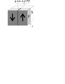
Figure 1: The superconductor ferromagnet junction. The domain wall.

$$\Gamma_{A}^{S\leftarrow F}(V)=4\pi^{3}\int d\xi n_{F}(\xi-eV)n_{F}(-\xi-eV)\times\\ \frac{\Delta^{2}}{[\Delta^{2}-\xi^{2}]}\sum_{\sigma}\tilde{\Xi}_{\sigma}(2\sqrt{\Delta^{2}-\xi^{2}}),$$ (5)

where $n_{F}(\xi)$ is the Fermi distribution function. Here and below describing the calculations we believe that $\hbar=1$. The $\Gamma_{A}^{S\rightarrow F}(V)$ can be obtained from the expression for $\Gamma_{A}^{S\leftarrow F}(V)$ by substitution $1-n_{F}$ for $n_{F}$. In derivation of Eq.(5) we assumed that the applied voltage is much smaller than the exchange energy, $|eV|\ll E_{\rm ex}$, and the ferromagnet is strongly polarized, $\nu_{\parallel}\gg\nu_{\nparallel}$. The conditions allow us to neglect contributions to the conductance due to the interference HekkingNazarov in the ferromagnet.

The kernel $\tilde{\Xi}_{\sigma}(s)\equiv\int_{0}^{\infty}dt\Xi_{\sigma}(t)e^{-st}$ is the Laplace transform of $\Xi_{\sigma}(t)$. It can be expressed through the classical probability $P(X_{1},\hat{p}_{1};X_{2},\hat{p}_{2},t)$ that an electron with the momentum directed along $\hat{p}_{1}$ initially situated at the point $X_{1}$ near the SF boundary arrives at time $t$ at some point $X_{2}$ near the SF boundary with the momentum directed along $\hat{p}_{2}$ spreading in the superconducting region as follows

$$\Xi_{\sigma}(t)=\frac{1}{8\pi^{3}e^{4}\nu_{S}}\int d\hat{p}_{1,2}\int dX_{1,2}P(X_{1},\hat{p}_{1};X_{2},\hat{p}_{2},t)\times\\ \left\{G(X_{1},\hat{p}_{1},\sigma)G(X_{2},\hat{p}_{2},\sigma)\sin^{2}\left(\frac{\theta(X_{1},X_{2})}{2}\right)+\right.\\ +\left.G(X_{1},\hat{p}_{1},\sigma)G(X_{2},\hat{p}_{2},-\sigma)\cos^{2}\left(\frac{\theta(X_{1},X_{2})}{2}\right)\right\}.$$ (6)

Here the spatial integration is performed over the surface of the SF junction. We choose the spin quantization axis in the direction of the local magnetization. The quasiclassical probabilities $G(X,\hat{p},\sigma)$ for the electron with spin polarization $\sigma$ to tunnel from the ferromagnet to the superconductor are normalized in such a way that the junction normal conductance per unit area $g_{\sigma}(X)$ and the total normal conductance $G_{N}$ are determined as HekkingNazarov ; AverinNazarov

$$g_{\sigma}(X)=\int d\hat{p}G(X,\hat{p},\sigma),\quad G_{N}=\int dX\sum\limits_{\sigma}g_{\sigma}(X).$$ (7)

Then the normal conductance per unit area discussed above is defined as $g_{N}=G_{N}/{\cal A}$, where ${\cal A}$ is the surface area of the SF interface. Symbol $\theta(X_{1},X_{2})$ is the angle between the magnetizations of the ferromagnet at points $X_{1}$ and $X_{2}$ near the SF boundary. In the limiting case of the monodomain ferromagnet (so $\theta(X_{1},X_{2})\equiv 0$) and weak spin polarization ($\nu_{\parallel}\approx\nu_{\nparallel}$) Eqs. (4)-(6) coincide with the results of Ref. HekkingNazarov and describe contribution to the subgap conductivity of a superconductor – normal metal junction due to the interference in the superconductor. Eqs.(4)-(6) describe the subgap current through the SF junction with general domain structure of the ferromagnet. For the SF junction with the monodomain fully polarized ferromagnet the subgap current vanishes according to Eqs.(4)-(6). However, inelastic processes provide small but nonlinear contribution to the subgap current which is asymmetric with the respect to the sign of the bias voltage Falko .

When the applied voltage is small, $|eV|\ll\Delta$, then the current is proportional to the voltage, $I(V)=G_{A}V$. At low temperature compared to the critical temperature of the superconductor, $T\ll T_{c}$, Eqs.(4)-(5) reduce to

$$G_{A}=8\pi^{3}e^{2}\sum_{\sigma}\tilde{\Xi}_{\sigma}(2\Delta).$$ (8)

Andreev conductance of a single domain wall.

The most interesting case is the fully polarized ferromagnet because then the Andreev conductance of the SF junction is completely determined by the contribution of domain walls. First we consider the SF junction with the ferromagnet consisting of two domains as shown in Fig. 1. If we choose the frame of reference according to Fig. 1 then the angle of magnetization rotates as follows Landau8

$$\theta(x,-\infty)=\arccos\tanh\frac{x}{\delta},$$ (9)

$$\theta(x_{1},x_{2})=\theta(x_{1},-\infty)-\theta(x_{2},-\infty).$$ (10)

The classical probability $P(X_{1},\hat{p}_{1};X_{2},\hat{p}_{2},t)$ is different in the dirty and clean superconductors. We consider therefore these cases separately.

When the superconductor is dirty we can neglect the momentum dependence of the classical probability $P(X_{1},\hat{p}_{1};X_{2},\hat{p}_{2},t)$, then

$$P(X_{1},X_{2},t)=\frac{2}{(4\pi Dt)^{3/2}}\exp\left[-\frac{(X_{1}-X_{2})^{2}}{4Dt}\right],$$ (11)

where the factor of $2$ appears because the superconductor occupies the half-space. Now we can integrate over the momentum directions $\hat{p}_{i}$ in Eq.(6). Believing that $g_{\sigma}(X)$ is a slow varying function of $X$ on the lengthscale $\max\{\xi_{0},\delta\}$ we can perform the integrations over the SF interface in Eq.(6) and obtain

$${\tilde{\Xi}}_{\sigma}(s)=\frac{L_{D}^{(\rm tot)}}{4\pi^{4}e^{4}\nu_{s}s}g_{\sigma}(g_{\sigma}-g_{-\sigma})F_{d}\left(\delta\sqrt{\frac{s}{D}}\right)+\\ +\frac{{\cal A}}{8\pi^{3}e^{4}\nu_{s}\sqrt{sD}}g_{\sigma}g_{-\sigma}.$$ (12)

Here the function $F_{d}(z)$ is defined as

$$F_{d}(z)=\int\limits_{0}^{\infty}dxK_{0}(x)x\tanh\left(\frac{x}{2z}\right),$$ (13)

where $K_{0}(x)$ is the modified Bessel function of the second kind.

With a help of Eqs. (8) and (12) we find that the Andreev conductance of the SF junction can be written as

$$G_{A}=G_{A}^{(0)}+G_{A}^{(D)},$$ (14)

where the surface and domain wall contributions are given by

$$G_{A}^{(0)}=\frac{4{\cal A}}{\pi e^{2}\nu_{s}\Delta\xi_{0}}g_{\uparrow}g_{\downarrow},$$ (15)

$$G_{A}^{(D)}=\frac{L_{D}^{(\rm tot)}}{\pi e^{2}\nu_{s}\Delta}\left(g_{\uparrow}-g_{\downarrow}\right)^{2}F_{d}\left(\frac{4\delta}{\pi\xi_{0}}\right).$$ (16)

The surface contribution $G_{A}^{(0)}$ is suppressed in the case of the fully polarized ferromagnet, $g_{\uparrow}\gg g_{\downarrow}$, and the domain wall contribution $G_{A}^{(D)}$ is the only that survives.

In the most interesting cases the function $F_{d}(z)$ has the following asymptotic behavior

$$F_{d}(z)=\begin{cases}1+\displaystyle\frac{\pi^{2}z^{2}}{12}\left(\ln z+1+\frac{6}{\pi^{2}}\zeta^{{}^{\prime}}(2)\right),&\text{$z\ll 1$},\\ \displaystyle\frac{\pi}{4z}\left(1+\frac{3}{4z^{2}}\right),&\text{$z\gg 1$}.\end{cases}$$ (17)

where $\zeta^{{}^{\prime}}(z)$ is the derivative of the Riemann zeta function. By using Eqs.(8),(16) and (17) for the case of the fully polarized ferromagnet, $g_{\downarrow}=0$, we obtain the result (1).

In the case of the clean superconductor we can estimate the classical probability as

$$P(X_{1},X_{2},t)=\frac{2}{4\pi(X_{1}-X_{2})^{2}}\delta(|X_{1}-X_{2}|-v_{F}t).$$ (18)

This probability describes tunneling through disordered SF boundary. It allows to reproduce Chtch-Marenko_Nazarov the results of Ref.  Falci_Feinberg_Hekking .

In a similar way as above we obtain

$${\tilde{\Xi}}_{\sigma}(s)=\frac{L_{D}^{(\rm tot)}}{4\pi^{4}e^{4}\nu_{s}s}g_{\sigma}(g_{\sigma}-g_{-\sigma})F_{c}\left(\frac{2\delta s}{v_{F}}\right)+\\ +\frac{\cal A}{8\pi^{3}e^{4}\nu_{s}v_{F}}g_{\sigma}g_{-\sigma}\left(\ln\frac{v_{F}}{\lambda_{F}s}-\gamma\right),$$ (19)

where $\gamma\approx 0.577$ is the Euler constant and the function $F_{c}(z)$ is defined as

$$F_{c}(z)=\int\limits_{0}^{\infty}dxK_{0}(x)\ln\cosh\frac{x}{z}.$$ (20)

Then, the surface and domain wall contributions to the Andreev conductance are as follows

$$G_{A}^{(0)}=\frac{2{\cal A}}{\pi e^{2}\nu_{s}\Delta\xi_{0}}g_{\uparrow}g_{\downarrow}\left(\ln\frac{\xi_{0}}{\lambda_{F}}-\gamma\right),$$ (21)

$$G_{A}^{(D)}=\frac{L_{D}^{(\rm tot)}}{e^{2}\nu_{s}\Delta}\left(g_{\uparrow}-g_{\downarrow}\right)^{2}F_{c}\left(\frac{4\delta}{\pi\xi_{0}}\right),$$ (22)

where $\lambda_{F}$ denotes the Fermi length. The function $F_{c}(z)$ has the following asymptotic behavior

$$F_{c}(z)=\begin{cases}1-\displaystyle\frac{\pi z}{2}\ln 2,&\text{$z\ll 1$},\\ \displaystyle\frac{\pi}{4z}\left(1+\frac{3}{z^{2}}\right),&\text{$z\gg 1$},\end{cases}$$ (23)

For the case of the fully polarized ferromagnet, $g_{\downarrow}=0$, Eqs.(8),(22) and (23) lead to the result (1).

Andreev conductance of several domain walls.

Now we consider the domain structure with several domain walls touching the SF interface. If domain walls separate domains with the opposite directions of magnetization then the Andreev conductance is a sum of contributions from each domain wall. By assuming that the characteristic domain size is much larger than the domain wall width and the magnetization rotation is given by Eq.(9), we find the result (1) with $L_{D}^{(\rm tot)}$ being the total length of the domain walls at the SF interface. Usually, the domain structure at the SF interface is more complicated. Nevertheless, the Andreev conductance remains proportional to the total domain wall length whereas the function $f(x)$ (see Eq.(1)) may depend on the particular domain structure.

Possible experimental setup can be prepared in a similar way as in recent experiment Ryazanov_vortices . The normal conductance between the superconductor and the ferromagnet should be smaller than the normal conductances of the leads and the ferromagnet (superconductor). The condition allows to neglect voltage gradients in the ferromagnet and believe that the ferromagnet is in equilibrium and that we measure The Andreev conductance of the SF junction rather than lead-related effects. By changing the applied magnetic field we would change the number of domains in the ferromagnet. As Eq.(1) shown, the Andreev conductance is proportional to the number of domain walls in the ferromagnet and, consequently, to the number of domains. It can be checked experimentally by measuring the Andreev conductance as a function of the applied magnetic field.

In conclusion, we evaluated the low-voltage Andreev conductance of the SF junction when the ferromagnet is strongly polarized and consists of several domains. The main transport mechanism under subgap conditions is two electron tunneling (with zero total spin of an electron pair) whereas the transfer of single electrons is strongly suppressed. Exchange field of the ferromagnet aligns electron spins and suppresses the two electron tunneling. However the tunneling is not suppressed near the domain walls where electrons involved come from (or come to) the adjacent domains. It is found that at strong polarization of the ferromagnet the domain wall contribution to the Andreev conductance is the largest. We presented an approach which gives an opportunity to find the subgap current in wide range of layouts. Dynamics of domains with magnetic field can be probed experimentally through the SF conductance measurement.

We are especially grateful to V.V. Ryazanov for suggesting the problem treated in this letter and stimulating discussions. Furthermore we thank M.V. Feigelman, A.S. Iosselevich, S. Koshuba and Ya. Fominov for useful discussions. We wish to thank RFBR (projects No. 03-02-06259, 03-02-16677, and 03-02-17494), the Netherlands Organization for Scientific Research (NWO), the Swiss NSF, Forschungszentrum Jülich (Landau Scholarship), the programs of the Russian Ministry of Science: Mesoscopic systems and Quantum computations and the program of the leading scientific schools support.

References

- (1) L. N. Bulaevskii, V. V. Kuzii, and A. A. Sobyanin, Pis’ma Zh. Eksp. Teor. Fiz. 25, 314 (1977) [JETP Lett. 25, 290 (1977)];
- (2) A. V. Veretennikov, V. V. Ryazanov, V. A. Oboznov, Physica B 284-288, 495 (2000); V. V. Ryazanov, V. A. Oboznov, A. Yu. Rusanov, Phys. Rev. Lett. 86, 2427 (2001).
- (3) N.M. Chtchelkatchev, W. Belzig, Yu.V. Nazarov, and C. Bruder, JETP Letters, 74, 323 (2001)
- (4) Ya. Fominov, N.M. Chtchelkatchev, and S. Golubov, JETP Lett. 74, 96 (2001) [Pis ma v Zh. Eksp. Teor. Fiz., 74, 101 (2001)].
- (5) E.B. Sonin, Phys. Rev. B 66, 100504(R), (2002); E. B. Sonin, cond-mat/0102102; E.B. Sonin, cond-mat/0202193
- (6) S. Erdin, A.F. Kayali, I. F. Lyuksyutov, and V. L.Pokrovsky, Phys. Rev. B 66, 014414 (2002); I. F. Lyuksyutov and V. L.Pokrovsky, cond-mat/9903312.
- (7) R.J. Kinsey, G. Burnell, and M.J. Blamir, IEEE Trans. Appl. Superc. 11, 904 (2001)
- (8) V. V. Ryazanov, V. A. Oboznov, A. S. Prokofiev, and S. V. Dubonos, JETP Lett. 77, 39 (2003) [Pis ma v ZhETF, 77, 43 (2003)]
- (9) A.F. Andreev, Sov. Phys. JETP 19, 1228 (1964)
- (10) G. Tkachov, E. McCann and V. I. Fal’ko, Phys. Rev. B 65, 024519 (2002).
- (11) F.W.J. Hekking and Yu.V. Nazarov, Phys. Rev. B 49, 6847 (1994)
- (12) D.V. Averin and Yu.V. Nazarov, Phys. Rev. Lett. 65, 2446 (1990)
- (13) L.D. Landau and E.M. Lifshitz, in Electrodynamics of Continious Media, Course in Theoretical Physics Vol. 8 (Pergamon Press, Oxford, 1984).
- (14) N.M. Chtchelkatchev, M. Mar’enko, and Yu. Nazarov, in preparation
- (15) G. Falci, D. Feinberg, F. W. J. Hekking, Europhys. Lett. 54, 225 (2001);