Effect of ion hydration on the first-order transition in the sequential wetting of hexane on brine

Abstract

In recent experiments, a sequence of changes in the wetting state (‘wetting transitions’) has been observed upon increasing the temperature in systems consisting of pentane on pure water and of hexane on brine. In this sequential-wetting scenario, there occurs a first-order transition from a partial-wetting state, in which only a microscopically thin film of adsorbate is present on the substrate, to a ‘frustrated complete wetting state’ characterized by a mesoscopically, but not yet macroscopically thick wetting film. At higher temperatures, one observes a continuous divergence of the film thickness and finally, at the critical-wetting temperature, the complete-wetting state, featuring a macroscopic film thickness, is reached. This sequence of two transitions is brought about by an interplay of short-range and long-range interactions between substrate and adsorbate. The critical wetting transition is controlled by the long-range forces and is, thus, found by determining where the Hamaker constant, as calculated from a Dzyaloshinskii–Lifshitz–Pitaevskii-type theory, changes sign. The first-order transition involves both short-range and long-range forces and is, therefore, more difficult to locate. While the pentane/water system is well understood in this respect by now, a detailed theoretical description of the hexane/brine system is hampered by the a priori unknown modification of the interactions between substrate and adsorbate upon the addition of salt. In this work, we argue that the short-range interaction (contact energy) between hexane and pure water remains unchanged due to the formation of a depletion layer (a thin ‘layer’ of pure water which is completely devoid of ions) at the surface of the electrolyte and that the presence of the salt manifests itself only in a modification of the long-range interaction between substrate and adsorbate. In a five-layer calculation considering brine, water, the first layer of adsorbed hexane molecules, liquid hexane, and vapor, we determine the new long-range interaction of brine with the adsorbate across the water ‘layer’. According to the recent theory of the excess surface tension of an electrolyte by Levin and Flores-Mena, this water ‘layer’ is of constant, i.e. salt-concentration independent, thickness $\delta$, with $\delta$ being the hydrodynamic radius of the ions in water. Once this radius has been determined, the first-order transition temperatures can be calculated from the dielectric properties of the five media. Our results for these temperatures are in good agreement with the experimental ones.

PACS: 05.70.Fh; 68.10.-m; 68.10.Cr; 68.45.Gd
Keywords: Wetting, Surface tension, Electrolytes

I. INTRODUCTION

Imagine a volatile substance, the adsorbate, to be at liquid–vapor coexistence and in contact with a third phase, the substrate, which might be solid or liquid. There are two qualitatively different ways in which the three phases can meet: one possibility, known as partial wetting, is that the liquid phase of the adsorbate forms discrete droplets on the surface of the substrate, which have non-zero contact angle with this surface. In this case, the droplets are connected only by a microscopically thin film of adsorbate that covers the substrate. According to Young’s equation [1], the contact angle $\theta$ is related to the three interfacial tensions between substrate and liquid ($\gamma_{sl}$), substrate and vapor ($\gamma_{sv}$), and liquid and vapor ($\gamma_{lv}$) and can be calculated from $\gamma_{sv}-\gamma_{sl}=\gamma_{lv}\cos{\theta}$. The second possible arrangement of the three phases is that the liquid phase forms a macroscopically thick layer on the substrate surface in such a way that there is no direct contact of substrate and vapor anymore. This situation is known as complete wetting and the three interfacial tensions obey Antonow’s rule: $\gamma_{sv}-\gamma_{sl}=\gamma_{lv}$. From this relation, it follows immediately that the contact angle $\theta$ is zero for complete wetting. In his seminal article on this subject, Cahn [2] demonstrated the possibility of a transition between the two states, partial and complete wetting, as, for example, the temperature is varied. He predicted that, close enough to the liquid–vapor critical point of the adsorbate, there will be a wetting transition from partial to complete wetting (or drying). His theory also predicts this transition to be of first-order nature – by now, it has been shown experimentally that this is usually the case for wetting transitions [3, 4, 5, 6, 7]. The discontinuous nature of the transition manifests itself in the abrupt jump of the layer thickness at the transition temperature $T_{w,1}$, in the existence of a prewetting line [5, 6, 7], and in the occurrence of hysteresis, one of the hallmarks of first-order transitions [4, 5].

Nevertheless, since the early days of the theory of wetting, there had been speculations about the possibility of a critical (or higher-order) wetting transition, in which the wetting-layer thickness diverges continuously to a macroscopic value [8, 9, 10, 11, 12, 13, 14]. In this context, it is important to distinguish between long-range and short-range critical wetting. For the latter, the film thickness is predicted to diverge logarithmically [8, 11, 14] (within mean-field theory), whereas, for the former, a power-law behavior according to the relation $l\sim\Delta T^{-1}$, where $l$ is the film thickness and $\Delta T=T_{w,c}-T$ measures the distance from the critical-wetting temperature, is expected [9, 10, 13, 15]. While the upper critical dimensionality for long-range critical wetting is less than three, which implies that the predictions of a mean-field theory are valid, it is equal to three for short-range critical wetting [11, 12, 13]. In contrast to long-range critical wetting, the occurrence of short-range critical wetting requires the proximity of a bulk critical point [8, 11].

While short-range critical wetting has been seen very recently in methanol/$n$-nonane mixtures [16], the first experimental observation of critical wetting was for an example of the long-range type: Ragil et al. reported a continuous divergence of the film thickness for pentane on water [17]. From the effective exponent of $-1$ that describes this divergence (see above) and the fact that the location of the transition (53^∘C) coincides with the temperature at which the Hamaker constant changes sign, it was concluded that long-range forces bring about the critical transition [17]. In accord with this assumption is the considerable distance of the critical wetting temperature from any bulk critical point.

For the system of hexane on pure water, i.e. for a three-layer configuration of the form water/liquid hexane/vapor, the critical-wetting temperature was estimated – based on calculations of the Hamaker constant – to be $T_{w,c}=96^{\circ}$C and is, therefore, too high to be observed using the existing experimental set-up [18]. In order to depress the (critical-)wetting temperature, salt (NaCl) was added to the system. [18, 19, 20] Interestingly, for salt concentrations of 1.5 mol/L and 2.5 mol/L, two marked changes of the film thickness were observed ellipsometrically [18]: at low temperatures, the adsorbed film is only a few Å thick; on passing the temperature $T_{w,1}$, there is an abrupt increase of the film thickness to about 100 Å. The hysteresis which is observed for this transition corroborates that this change of the wetting state is of first-order nature. Upon increasing the temperature further, the film thickness grows continuously and diverges at $T_{w,c}$, just as it had been observed for pentane on water. Returning to the pentane/water system, it was found that, when heating the system from low temperatures instead of cooling it down from $T_{w,c}$, as had been done before, a first-order thin–thick transition occurs at 25^∘C in this system as well [21].

On the basis of the conventional Cahn theory, the first-order transition in this system was predicted to occur at $-30^{\circ}$C [22]; a modification of the original theory by Dobbs [23], however, which treats the first layer of adsorbate molecules in a lattice-gas approximation and, thereby, fulfills Henry’s law, brought the estimate of $T_{w,1}$ closer to 25^∘C (or, to be more precise, to within the range 13–70^∘C, depending on the effective diameter of a pentane molecule that one assumes. Adopting a value of 4.4 Å, which follows from the excluded volume used in the Peng–Robinson equation of state, yields $T_{w,1}=38^{\circ}$C.) [21, 23].

Within this theoretical setting, the observed sequence of wetting transitions (‘sequential wetting’) is brought about by the interplay of short-range and long-range forces. At low temperatures, both long-range and short-range interactions inhibit the formation of a wetting layer. At $T_{w,1}$ (the wetting temperature predicted by Cahn theory based on short-range forces alone), the short-range forces start to favor a wetting layer (in a sense that the gain in free energy from having such a layer outweighs the cost of creating an additional liquid–vapor interface), the long-range forces, however, still act against the formation of a macroscopically thick film; the result of this interplay is a compromise: the mesoscopically thick film, which is present in an intermediate wetting state that has been termed ‘frustrated-complete wetting’ [21]. At $T_{w,c}$, the effect of long-range forces changes its nature from inhibiting to supporting a thick wetting layer and, consequently, the layer thickness diverges.

This interplay also illustrates why sequential wetting has been observed only for such a small number of systems: the window of opportunity for it to occur is relatively narrow, and, in most cases, the long-range forces will support wetting before the short-range forces do, so that only a first-order wetting transition is observed at the temperature at which the short-range forces start to favor wetting (as in standard Cahn theory).

As already mentioned, the location of the critical-wetting transition is relatively easily calculated from the variation of the Hamaker constant as a function of temperature. Within Israelachvili’s approximation [24], only the static dielectric constants, the refractive indices, and a typical absorption frequency of the substances involved are required.

The location of the first-order thin–thick transition, however, is more difficult to predict: within a Cahn-type theory, knowledge of the so-called contact energy, which describes the short-range interaction between substrate and adsorbate (as deduced from measurements of the surface pressure, for example [22]) is needed. Furthermore, the conventional Cahn theory underestimates the (first-order) wetting temperature of alkanes on water considerably [22] – only a modification introduced by Dobbs [23] allows one to predict $T_{w,1}$ (semi-)quantitatively, but it requires an effective diameter of the adsorbate molecule on the assumption that the latter is spherical [21, 23].

For pentane on water, it has been shown that this kind of theory, when combined with appropriate expressions for the amplitudes of the long-distance tails of the long-range forces [25], is able to reproduce both wetting-transition temperatures accurately, $T_{w,1}=298$ K and $T_{w,c}=326$ K. [26] Note, however, that, using the same parameters, the short-range forces alone (Dobbs’ theory) would predict $T_{w,1}=311$ K, so the long-range forces are not qualitatively, but, to some degree, quantitatively important also for the first-order transition.

Another unexpected finding in the experiments on the hexane/brine system, in addition to the occurrence of sequential wetting, was that the two transition temperatures, $T_{w,1}$ and $T_{w,c}$, were shifted in parallel as a function of the salt concentration [18]. On theoretical grounds, it had been expected that the (critical) wetting temperature decreases with increasing salinity of the substrate [19]. This behavior is indeed observed in the experiments [18]. The first-order transition temperature, however, was expected [18, 27] to remain largely unchanged because the brine/air(vapor) and brine/alkane interfacial tensions vary in a similar fashion as a function of the salt concentration [28]. It was even hoped that the two lines of transition temperatures would meet to form a critical endpoint [27] (like in a simple model system of sequential wetting [29]) – this expectation, however, was not met: as already mentioned, the two lines run in parallel and, at first glance, the two transition temperatures might appear coupled [18, 30]. (In contrast to the situation at $T_{w,c}$, which is necessarily the temperature at which the Hamaker constant $W$ changes sign, there is nothing peculiar or exceptional about the behavior of $W$ at $T_{w,1}$, a temperature which is not determined by the long-range forces alone. [21, 31]) In an attempt to illustrate that $T_{w,1}$ (or at least $\Delta T_{w,1}$, the shift of $T_{w,1}$ as compared to the case of hexane on pure water) is determined by the same dielectric properties as $T_{w,c}$, Bertrand et al. proposed a Dzyaloshinskii–Lifshitz–Pitaevskii(DLP)-type theory [32] to calculate the change in contact energy between substrate and adsorbate on addition of salt for the system of hexane on brine[30]. With the aid of a Cahn phase portrait (for hexane on pure water, neglecting long-range forces), the contact-energy difference is then converted into a shift of the first-order transition temperature. The DLP-type calculation takes into account the existence of a depletion layer at the brine/alkane interface, which is almost completely devoid of ions [28, 33, 34]. The calculation of the free energy per unit area therefore involves four layers: brine/water/liquid alkane/vapor [30]. If the thickness of the water layer is assumed to be 2 Å, which is consistent with estimates based on the Onsager–Samaras theory of the interfacial tension of electrolytes [33], which attributes the ions being repelled from the interface to electrostatic effects due to image charges, one obtains first-order wetting temperatures that are in very good agreement with the experimental results [30]. Since the thickness $\delta$ does not depend on the Hamaker constant, this actually just demonstrates that DLP theory works even on very short length scales, for which it was not designed originally, but in no way does it support the supposition that the Hamaker constant might determine $T_{w,1}$ as well.

Within Onsager–Samaras theory, however, $\delta$ is a function of the salt concentration $c_{\rm NaCl}$, as Bertrand et al. pointed out [33, 30]. If this dependence is taken into account, the agreement of the calculated $T_{w,1}$ with the experimental values deteriorates quickly as $c_{\rm NaCl}$ increases. Bertrand et al. speculatively attribute this behavior to the breakdown of the underlying Debye–Hückel theory for higher concentrations [30].

In this paper, we take a somewhat different view and develop a theory that – also based on DLP theory – accounts for the modifications of the long-range forces due to the presence of salt. The system we consider is similar in spirit to the four-layer structure (brine/water/liquid alkane/vapor); in order to have a complete description of our system within the theoretical framework, we also take into account the first layer of adsorbed hexane molecules, which is denser than the bulk liquid hexane, as a separate, fifth medium and, thus, deal with a five-layer structure (brine/water/dense liquid hexane/liquid hexane/vapor). To estimate the thickness of the layer of pure water, $\delta$, however, we do not rely on Onsager–Samaras theory, which is not valid in the concentration range of interest here (0.5 mol/L $\leq c_{\rm NaCl}\leq$ 2.5 mol/L), but only up to $c_{\rm NaCl}\approx 0.15$ mol/L [35]. Instead, we adopt an idea that has recently been advanced by Levin and Flores-Mena in order to improve upon Onsager–Samaras theory for higher salt concentration [36]. They had realized that – in addition to the effect of an electrostatic repulsion of the ions from the interface – there is a concentration-independent depletion layer, the thickness of which corresponds to the radius of the hydrated ion, which is also about $\delta=2$ Å for NaCl [36, 37]. Therefore, the apparent puzzle of having a constant thickness of the depletion layer is not due to the breakdown of Debye–Hückel theory (which seems to work fine even for relatively high concentrations of 1 mol/L in the theory of Levin and Flores-Mena [36]), but is due to the omission of the effect of the hydration-sphere contribution in Onsager–Samaras theory. This theory had been designed for the low-concentration regime, in which the depletion-layer thickness is dominated by electrostatic effects, whereas it is the hydrodynamic ionic radius that sets $\delta$ for the concentration range in which we are interested here.

Now we argue that the contact energy in the hexane/brine system is still the same as in the hexane/pure-water case because, as before, only pure water is in direct contact with the adsorbed hexane. What changes upon the addition of salt is the long-range interaction between the substrate, now brine, and the adsorbate, hexane, across the water ‘layer’ of constant thickness $\delta$. Based on these insights, we will develop a new theory to compute the first-order wetting temperatures.

The remainder of the paper is organized as follows: in the next section, we will explain our approach in detail. The results of our calculations will be presented in Sec. III. A discussion of the results and of future tasks in Sec. IV will conclude the article.

II. METHODOLOGY AND OUTLINE OF THE THEORY

This section contains the theoretical framework by means of which we describe the wetting properties of an alkane (hexane in this case) on pure water and on brine, respectively. First, we will briefly summarize the equation of state that is used to represent and compute the bulk properties of hexane. The fact that hexane and (salt) water are hardly miscible allows us to use an equation of state for the pure adsorbate and enables us to manage without an equation of state for the substrate. In the second subsection, we present the modified Cahn–Landau model for the interfacial tensions, which, in turn, determine the wetting properties. In that subsection, we will also give a detailed account of how the long-range field is modified by the presence of salt and of a depletion layer. For completeness and reproducibility, we also list the representative equations for the dielectric properties of all five media involved. A third subsection will contain some of the technical details of our calculations.

A. Equation of state for hexane

As in several previous works on the wetting properties of alkanes (on aqueous substrates) [17, 23, 22, 26], we employ the Peng–Robinson equation of state to describe the thermophysical bulk properties of hexane [38]. According to this equation of state, the pressure is given by:

$$P=\frac{\rho RT}{1-b\rho}+\frac{a(T)\rho^{2}}{1+b\rho(2-b\rho)},$$ (1)

where $T$ is the absolute temperature, $R$ the molar gas constant, and $\rho$ the molar density. The excluded volume $b$ is determined from critical parameters (see below), while the function $a(T)$ also involves the vapor pressure at the reduced temperature $t=T/T_{c}=0.7$. Adopting Peng and Robinson’s recommendations, we use the following prescriptions for the above-mentioned parameters:

$$b = 0.07780\,RT_{c}/P_{c},$$ (2)

$$a(T) = a(T_{c})\alpha(t,\omega),$$ (3)

$$a(T_{c}) = 0.045724\,(RT_{c})^{2}/P_{c}.$$ (4)

In the second equation, $\omega$ is the acentric factor given by

$$\omega=-1-\log_{10}{\left[P(t=0.7)/P_{c}\right]};$$ (5)

the function $\alpha(t,\omega)$ is defined as

$$\alpha(t,\omega) = \left[1+K(\omega)\left(1-t^{1/2}\right)\right]^{2}$$ (6)

$$K(\omega) = 0.37464+1.54226\,\omega-0.26992\,\omega^{2}.$$ (7)

The critical and other required parameters for hexane are [39, 40]:

$$T_{c} = 507.7\,{\rm K}$$ (8)

$$P_{c} = 3.010\,{\rm MPa}$$ (9)

$$\omega = 0.296.$$ (10)

B. Model for the interfacial tension

Here, we distinguish between two cases and present the theories to describe the wetting behavior of hexane on pure water and on brine separately.

1. Hexane on pure water

For hexane on pure water, we use a model of the interfacial tension that is completely analogous to the one employed by Weiss and Widom for pentane on water [26]. This model, in turn, is a combination of Dobbs’ modified Cahn theory [23] and a treatment of the algebraic tails of the long-range forces as proposed by Indekeu et al. [25] Within this model, the interfacial tension is obtained by minimizing the free-energy functional with respect to the density profile of the adsorbate, $\rho(z)$, in conjunction with the appropriate boundary conditions (see Sec. II.C for details). The free-energy functional reads:

$$\gamma[\rho] = \gamma_{0}+\phi(\rho_{0})+\int\limits_{\Delta z}^{\infty}\left\{\Delta f(\rho,\rho_{bulk})+\frac{c}{2}\left(\frac{d\rho}{dz}\right)^{2}\right\}dz$$ (11)

$$+\left\{\Delta f(\rho_{0},\rho_{bulk})+\frac{c}{2}\left[(\rho_{0}-\rho_{1})/\Delta z\right]^{2}\right\}\Delta z$$

$$-\int\limits_{z_{c}}^{\infty}\left(\frac{a_{3}}{z^{3}}+\frac{a_{4}}{z^{4}}\right)\rho(z)dz.$$

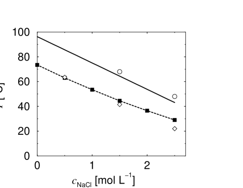
FIG. 2: First-order and critical-wetting transition temperatures for hexane on brine as a function of the salt concentration. The open circles denote the experimental critical-wetting temperatures [18], while the continuous line marks the theoretical prediction for this transition, as obtained from the temperature at which the Hamaker constant changes sign. The open diamonds represent the experimental first-order transition temperatures [18], and the filled squares, connected by the dashed line to guide the eye, are our theoretical predictions using a depletion-layer thickness of $\delta=1.9$ Å.

In this model, the $z$-axis is perpendicular to the substrate surface and the substrate (water) is assumed to occupy the lower half-space, for which $z<0$, so that the planar water/hexane interface is located at $z=0$. For $z>0$, $\rho(z)$ denotes the spatially varying density of hexane, while $\rho_{bulk}$ is the density of either bulk phase, liquid or vapor. The density of the adsorbate at the substrate surface, $\rho(z=0)$, is denoted by $\rho_{0}$. The first term, $\gamma_{0}$, represents that part of the interfacial tension that is due to the self-interaction of the substrate (water/vacuum), but since it is only a function of temperature and an additive term contributing equally to each interfacial tension (except for $\gamma_{lv}$, which does not involve the interaction with a substrate), it is irrelevant to the wetting properties of the adsorbate, and no value of $\gamma_{0}$ needs to be specified. In the second term, $\phi(\rho_{0})$ denotes the contact energy, which depends only on the surface density of the adsorbate. Within the framework of his modified Cahn theory, Dobbs [23] determined the contact energy for several $n$-alkanes on water from experimental data for the surface pressure, applying a procedure that had been proposed by Ragil et al. [22] using standard Cahn theory. For hexane on pure water, we find from Fig. 2 in Dobbs’ paper:

$$\phi(\rho_{0})=\left[-4.16\rho_{0}b+2.15(\rho_{0}b)^{2}\right]P_{c}\lambda.$$ (12)

Here, $\lambda$ is a characteristic length scale of the system (approximately 34 Å) defined by $\lambda=(c/(b^{2}P_{c}))^{1/2}$, where $c$ is the influence parameter (or simply the coefficient of the square-gradient term). By matching to the experimental surface tension data of $n$-alkanes, Carey et al. [41] found that $c$ can be estimated from the parameters $a$ and $b$ in the Peng–Robinson equation of state for $n$-alkanes of short and medium chain length (on the basis of a corresponding-states idea). Their relation reads [41]:

$$c=0.27N_{A}^{-2/3}ab^{2/3}+7.25\times 10^{-20}{\rm J\,m^{5}\,mol^{-2}}$$ (13)

with $N_{A}$ being Avogadro’s constant.

The third term in Eq. (11) is the continuum part from standard Cahn–Landau theory, where $\Delta f$ measures the excess free energy corresponding to the local density over that of either bulk phase. It is given by $\Delta f(\rho,\rho_{bulk})=f(\rho)-\rho\mu_{bulk}+P_{bulk}$; here, $f=F/V$ is the Helmholtz free-energy density, $\mu_{bulk}$ the bulk chemical potential, and $\rho$ the local density of hexane, $\rho(z)$. The coefficient $c$ is the influence parameter as given by Eq. (13). The integration is to be performed from $\Delta z$ to infinity in this case, where $\Delta z$ is the ‘thickness’ of the first layer of adsorbed hexane molecules [23]. Treating the hexane molecule as spherical and estimating its diameter $\sigma$ from the excluded-volume term in the Peng–Robinson equation of state, one obtains $\Delta z=\sigma=4.4$ Å[21]. The first layer of hexane molecules ($0<z<\Delta z$) is considered explicitly in a lattice-gas approach and contributes the fourth term to Eq. (11), which is a discretized version of the third. The density at a distance $\Delta z$ from the substrate is denoted by $\rho_{1}$.

The last term contains the long-range field, which – in a first approximation – couples linearly to the density. Following Indekeu et al., we adopt a lower cutoff of $z_{c}=0.2\lambda$, which worked well for pentane [25, 26]; for hexane as the adsorbate, we, therefore, have $z_{c}\approx 6.8$ Å. This value is also very close to $1.5\,\sigma\approx 6.6$ Å, the distance of closest approach of adsorbate particles that are not in the first layer, but part of the continuum in the modified Cahn theory. The amplitudes of the first couple of leading terms in a $1/z$-expansion of the long-range forces, $a_{3}$ and $a_{4}$, are calculated from DLP theory as follows: invoking Israelachvili’s approximation [24], which amounts to the assumption that all media involved have the same characteristic absorption frequency $\omega_{e}$ and that the dielectric spectrum of substance $j$ can be represented by $\varepsilon_{j}(i\zeta)=1+(n_{j}^{2}-1)/(1+(\zeta/\omega_{e})^{2})$, with $n_{j}$ being the refractive index and $\zeta$ denoting the frequency, the Hamaker constant of a water(1)/liquid hexane(3)/vapor(2) system is given by [24]:

$$W = \frac{3}{4}k_{B}T\,\left(\frac{\varepsilon_{3}(0)-\varepsilon_{1}(0)}{\varepsilon_{3}(0)+\varepsilon_{1}(0)}\right)\,\left(\frac{\varepsilon_{3}(0)-\varepsilon_{2}(0)}{\varepsilon_{3}(0)+\varepsilon_{2}(0)}\right)$$ (14)

$$+\frac{3\hbar\omega_{e}}{8\sqrt{2}}\frac{\left(n_{3}^{2}-n_{1}^{2}\right)\left(n_{3}^{2}-n_{2}^{2}\right)}{\left(n_{3}^{2}+n_{1}^{2}\right)^{1/2}\left(n_{3}^{2}+n_{2}^{2}\right)^{1/2}\left[\left(n_{3}^{2}+n_{1}^{2}\right)^{1/2}+\left(n_{3}^{2}+n_{2}^{2}\right)^{1/2}\right]}.$$

In this equation, $k_{B}$ is Boltzmann’s constant, while $\hbar$ denotes Planck’s constant. The coefficient $a_{3}$ is related to $W$ by $a_{3}=-W/(6\pi\rho_{l})$, where the denominator should actually contain the difference $\rho_{l}-\rho_{v}$, but in view of the large distance from the bulk critical point of hexane, $\rho_{v}$ can safely be neglected [25].

To calculate $a_{4}$, we follow the approach of Bertrand et al. [42, 43] and consider a four-layer structure water(1)/dense liquid hexane(4)/liquid hexane(3)/vapor(2) because, right at the water/hexane interface, there is a thin layer (of approximately one molecular diameter thickness) of hexane whose density is higher than the bulk liquid density at the respective temperature; cf. Fig. 1 (a). Since the layer of liquid hexane, the thickness of which we denote by $l$, is assumed to be much thicker than just one molecular diameter $\sigma$ in the frustrated-complete wetting state (and certainly so in the complete-wetting state), we expand the full free energy per unit area of the four-layer structure, as given by Mahanty and Ninham [44] and by Parsegian and Ninham [45], in powers of $\sigma/l$ and truncate the resulting series after the linear term, since $\sigma\ll l$. The Hamaker constant and, therefore, the expression for $a_{3}$ remain unchanged by this consideration: the $l^{-2}$-term gives the Hamaker constant just as in Eq. (14), while the $\sigma/l^{3}$-term results in a coefficient $B$ as appearing in the following expansion of the long-range part of the free energy per unit area:

$$\gamma_{\rm LR}(l,\sigma)=-\frac{W}{12\pi l^{2}}+\frac{B\,\sigma}{12\pi l^{3}},$$ (15)

where our result for $B$ is given by:

$$B = -\frac{3}{2}k_{B}T\,\left(\frac{\varepsilon_{3}(0)\left[\varepsilon_{1}(0)-\varepsilon_{4}(0)\right]\left[\varepsilon_{1}(0)+\varepsilon_{4}(0)\right]}{\varepsilon_{4}(0)\left[\varepsilon_{1}(0)+\varepsilon_{3}(0)\right]^{2}}\right)\,\left(\frac{\varepsilon_{3}(0)-\varepsilon_{2}(0)}{\varepsilon_{3}(0)+\varepsilon_{2}(0)}\right)$$ (16)

$$-\frac{3\hbar\omega_{e}}{4\sqrt{2}}\left(n_{3}^{2}-n_{2}^{2}\right)\left(n_{1}^{2}-n_{4}^{2}\right)A,$$

with $A$ being:

$$A = \frac{\left(n_{1}^{2}-n_{3}^{2}\right)\left(n_{3}^{2}-n_{4}^{2}\right)}{2\left(n_{1}^{2}-n_{2}^{2}\right)\left(n_{1}^{2}+n_{3}^{2}\right)^{3/2}\left(n_{1}^{2}+n_{3}^{2}-2n_{4}^{2}\right)}$$ (17)

$$+\frac{\sqrt{2}\left(n_{1}^{2}-n_{4}^{2}\right)\left(n_{3}^{2}-n_{4}^{2}\right)}{n_{4}\left(n_{1}^{2}+n_{3}^{2}-2n_{4}^{2}\right)^{2}\left(n_{2}^{2}+n_{3}^{2}-2n_{4}^{2}\right)}$$

$$+\frac{\left(n_{2}^{2}-n_{3}^{2}\right)\left(n_{1}^{2}-n_{2}^{2}-n_{3}^{2}+n_{4}^{2}\right)}{\left(n_{1}^{2}-n_{2}^{2}\right)^{2}\left(n_{2}^{2}+n_{3}^{2}\right)^{1/2}\left(n_{2}^{2}+n_{3}^{2}-2n_{4}^{2}\right)}$$

$$+\frac{-n_{1}^{6}+n_{1}^{4}\left(n_{2}^{2}+n_{3}^{2}+n_{4}^{2}\right)-n_{1}^{2}\left(n_{3}^{4}+2n_{2}^{2}n_{4}^{2}\right)}{\left(n_{1}^{2}-n_{2}^{2}\right)^{2}\left(n_{1}^{2}+n_{3}^{2}\right)^{1/2}\left(n_{1}^{2}+n_{3}^{2}-2n_{4}^{2}\right)^{2}}$$

$$+\frac{-n_{3}^{2}\left(n_{3}^{4}-3n_{3}^{2}n_{4}^{2}+2n_{4}^{4}\right)+n_{2}^{2}\left(n_{3}^{4}-2n_{3}^{2}n_{4}^{2}+2n_{4}^{4}\right)}{\left(n_{1}^{2}-n_{2}^{2}\right)^{2}\left(n_{1}^{2}+n_{3}^{2}\right)^{1/2}\left(n_{1}^{2}+n_{3}^{2}-2n_{4}^{2}\right)^{2}}.$$

We remark that, since $B$ is approximately of the same order of magnitude as $W$ ($10^{-20}$ J) far from $T_{w,c}$ (it is actually four times larger than $W$ at $T=0^{\circ}$C and ten times larger than $W$ at $T_{w,1}$), the second term in Eq. (15) is indeed typically smaller than the first by a factor of $\sigma/l$. In contrast, near $T_{w,c}$, $W$ is negligible and $B$ becomes all-important.

The amplitude $a_{4}$ is related to $B$ via $a_{4}=B\sigma/(4\pi\rho_{l})$, where again, $\rho_{v}$ has been neglected in the denominator since, far from the critical point of hexane, $\rho_{l}\gg\rho_{v}$. Table I contains the representative equations for the dielectric properties involved in the above expressions. The static dielectric constant and the refractive index of the hexane layer near the water surface is estimated using the Clausius–Mossotti and Lorenz–Lorentz equations, respectively, assuming that the density of hexane is enhanced by about 12% compared to the bulk density of the liquid [22, 42]. Numerically, the results for $B$ from the above expression are very close to those obtained from the corresponding relation derived by Bertrand et al. [42, 43], which, in addition to the truncated $\sigma/l$-expansion, assumes $\varepsilon_{3}\approx\varepsilon_{4}$ as well as $n_{3}\approx n_{4}$ and is, therefore, limited to quadratic order in the terms $\Delta_{jk}(i\zeta)$, where $\Delta_{jk}(i\zeta)=\left(\varepsilon_{j}(i\zeta)-\varepsilon_{k}(i\zeta)\right)/\left(\varepsilon_{j}(i\zeta)+\varepsilon_{k}(i\zeta)\right)$. This additional approximation does not allow one to recover the formally correct result for the Hamaker constant in this four-layer calculation. Bertrand’s approximate relation [42] reads:

$$B\approx\frac{3}{2}\,k_{B}T\Delta_{32}(0)\Delta_{41}(0)+\frac{3}{4\sqrt{2}}\,\hbar\omega_{e}N(3,2,4,1),$$ (18)

where

$$N(f,g,j,k)=\frac{\left(n_{f}^{2}-n_{g}^{2}\right)\left(n_{j}^{2}-n_{k}^{2}\right)}{\left(n_{f}^{2}+n_{g}^{2}\right)^{1/2}\left(n_{j}^{2}+n_{k}^{2}\right)^{1/2}\left[\left(n_{f}^{2}+n_{g}^{2}\right)^{1/2}+\left(n_{j}^{2}+n_{k}^{2}\right)^{1/2}\right]}.$$ (19)

In the following, we propose an alternative approach, which will prove advantageous in the next subsection concerning the case of hexane on brine. It, too, is a quadratic approximation in the quantities $\Delta_{jk}$ but recovers the exact limits for $\sigma\to 0$ and $\sigma\to\infty$. According to Mahanty and Ninham [44], the expression for $\Delta_{3;41}(\sigma)$ in a four-layer structure, in which medium 3 is of fixed thickness $l$, and media 1 and 3 are separated by an intervening layer of medium 4, whose thickness is $\sigma$ (cf. Fig. 1 (a)), reads (omitting the frequency-dependence of $\Delta$ for brevity)

$$\Delta_{3;41}(\sigma)=\frac{\Delta_{34}+\Delta_{41}e^{-\sigma x/l}}{1+\Delta_{34}\Delta_{41}e^{-\sigma x/l}},$$ (20)

where $x$ is a dimensionless variable of integration. Note that $\Delta_{3;41}(0)=\Delta_{31}$ and $\Delta_{3;41}(\infty)=\Delta_{34}$. In Bertrand’s approximation [42], which is conform with the expansion proposed by Mahanty and Ninham [44], this expression reduces to $\Delta_{3;41}(\sigma)\approx\Delta_{34}+\Delta_{41}e^{-\sigma x/l}$, which yields the exact result for $\sigma\to\infty$, but not for $\sigma\to 0$. In the limit $\sigma\to 0$, one has $\Delta_{3;41}(0)\approx\Delta_{34}+\Delta_{41}$, which is not exact but correct to order $\Delta^{2}$. We now observe that $\Delta_{41}=\Delta_{31}-\Delta_{34}+O(\Delta^{2})$, using Eq. (20) at $\sigma=0$. Replacing $\Delta_{41}$ by this expression in Eq. (20), we obtain $\Delta_{3;41}(\sigma)\approx\Delta_{34}+\left(\Delta_{31}-\Delta_{34}\right)e^{-\sigma x/l}$, which is correct to order $\Delta^{2}$ and yields the exact results in both limits $\sigma\to 0$ and $\sigma\to\infty$. It, therefore, allows one to obtain the exact Hamaker constant $W$ in addition to an expression for $B$ within an approximation to quadratic order in $\Delta_{jk}$, in the context of an expansion to first order in $\sigma/l$. The latter expression reads:

$$B\approx\frac{3}{2}\,k_{B}T\Delta_{32}(0)\left[\Delta_{31}(0)-\Delta_{34}(0)\right]+\frac{3}{4\sqrt{2}}\,\hbar\omega_{e}\left[N(3,2,3,1)-N(3,2,3,4)\right].$$ (21)

Numerically, Eqs. (18) and (21) give very similar results; to within a resolution of 0.5 K, there is no detectable difference in the resulting $T_{w,1}$.

In the actual process of minimizing the free-energy functional Eq. (11), we use representative equations for the amplitudes $a_{3}$ and $a_{4}$, which were obtained by linear regressions to the results of Eqs. (14) and (21), and which, for hexane on pure water, read:

$$a_{3} = \left(4.681\times 10^{-23}{\rm J\,K^{-1}}(T-273.15\,{\rm K})-4.460\times 10^{-21}{\rm J}\right)/\left(6\pi\rho_{l}\right)$$ (22)

$$a_{4} = \left(-5.432\times 10^{-32}{\rm Jm\,K^{-1}}(T-273.15\,{\rm K})+8.987\times 10^{-30}{\rm Jm}\right)/\left(4\pi\rho_{l}\right).$$ (23)

Using the above expressions, we obtain $T_{w,1}=346$ K and $T_{w,c}=369$ K in nearly perfect agreement with the values that were extrapolated from the experimental transition temperatures for hexane on brine using different concentrations of salt (2.5, 1.5, and 0.5 mol/L) down to $c_{\rm NaCl}=0$ mol/L [18].

2. Hexane on brine

As already mentioned in the introduction, the fact that ions dissolved in water carry a hydration sphere around them, which prevents the ionic centers from approaching the (salt) water/alkane interface any closer than the distance set by the radius of this sphere, creates a depletion ‘layer’ of pure water near this interface [36]. Despite the fact that DLP theory was derived for much larger separations (thicker films) than the molecular dimensions we are dealing with here, it seems to work reliably even in these extreme cases of very short length scales. With this additional ‘layer’ of pure water present, we now consider a five-layer structure consisting of brine(1)/water(4)/dense liquid hexane(5)/liquid hexane(3)/vapor(2); see Fig. 1 (b). In this calculation the brine and vapor phases are semi-infinite slabs, while the water layer is of thickness $\delta$. The layer of dense liquid hexane, again, has molecular dimensions set equal to the diameter $\sigma$ of a hexane molecule, and the film of liquid hexane is of thickness $l$.

The origin of the $z$-axis, which marks the border between substrate and adsorbate, is now located between the layer of pure water and the molecular layer of dense liquid hexane. Therefore, the major formal difference between layers (4) and (5) is that the water layer is part of the substrate ($z<0$, but this part is not considered explicitly in the free-energy functional), while the first layer of adsorbed hexane molecules clearly is part of the adsorbate ($z>0$). In the derivation of Eq. (16), it was assumed that $l$ is much larger than $\sigma$, so, strictly speaking, this approximation is applicable to the frustrated-complete and complete wetting states, but not to partial wetting. In this latter state, however, the cutoff $z_{c}$ being larger than $\sigma$ ensures that the substrate–adsorbate (dense liquid hexane, $z<\sigma$) interaction is entirely accounted for by the contact energy.

In the present five-layer calculation, the long-range interaction of the substrate (brine) with the adsorbate, not the one between the water layer and the adsorbate, however, now involves the additional distance $\delta$, the thickness of the intervening water layer. The complete expression for $\Delta_{3;451}(\delta,\sigma)$ with two intervening layers 4 and 5 of thickness $\delta$ and $\sigma$, respectively, now reads [44]:

$$\Delta_{3;451}(\delta,\sigma)=\frac{\Delta_{35}+\Delta_{5;41}(\delta)e^{-\sigma x/l}}{1+\Delta_{35}\Delta_{5;41}(\delta)e^{-\sigma x/l}},$$ (24)

where $\Delta_{5;41}(\delta)$ is given by

$$\Delta_{5;41}(\delta)=\frac{\Delta_{54}+\Delta_{41}e^{-\delta x/l}}{1+\Delta_{54}\Delta_{41}e^{-\delta x/l}}.$$ (25)

Analogously to what was done for $\Delta_{3;41}(\sigma)$ in the previous section, $\Delta_{5;41}(\delta)$ is now approximated by $\Delta_{5;41}(\delta)\approx\Delta_{54}+\left(\Delta_{51}-\Delta_{54}\right)e^{-\delta x/l}$, which is correct to order $\Delta^{2}$ and ensures proper behavior in the limits $\delta\to 0$ and $\delta\to\infty$. Thus, we have

$$\Delta_{3;451}(\delta,\sigma)\approx\frac{\Delta_{35}+\left[\Delta_{54}+\left(\Delta_{51}-\Delta_{54}\right)e^{-\delta x/l}\right]e^{-\sigma x/l}}{1+\Delta_{35}\left[\Delta_{54}+\left(\Delta_{51}-\Delta_{54}\right)e^{-\delta x/l}\right]e^{-\sigma x/l}}.$$ (26)

Taking the limits $\delta\to 0$ and $\sigma\to 0$ at the same time leads us to the identity $\Delta_{3;451}(0,0)=\left(\Delta_{35}+\Delta_{51}\right)/\left(1+\Delta_{35}\Delta_{51}\right)=\Delta_{31}$, from which we obtain – to quadratic order in $\Delta_{jk}$ – the approximation $\Delta_{51}\approx\Delta_{31}-\Delta_{35}$. Therefore, $\Delta_{3;451}(\delta,\sigma)$ now, again to quadratic order, becomes

$$\Delta_{3;451}(\delta,\sigma)\approx\Delta_{35}+\Delta_{54}\,e^{-\sigma x/l}+\left(\Delta_{31}-\Delta_{35}-\Delta_{54}\right)e^{-\left(\sigma+\delta\right)x/l}.$$ (27)

Note that this is exact in the two limits $\sigma\to\infty$ and $\sigma=\delta=0$. From here, we proceed by considering the limit $\delta\to\infty$, for which $\Delta_{3;451}(\delta,\sigma)$ must transform into $\Delta_{3;54}(\sigma)$. The resulting approximation for the remaining four-layer structure (4/5/3/2) is $\Delta_{3;54}(\sigma)\approx\Delta_{35}+\Delta_{54}e^{-\sigma x/l}$, which, in the limit $\sigma\to 0$, yields $\Delta_{54}\approx\Delta_{34}-\Delta_{35}$. Substituting this into Eq. (27), we arrive at

$$\Delta_{3;451}(\delta,\sigma)\approx\Delta_{35}+\left(\Delta_{34}-\Delta_{35}\right)e^{-\sigma x/l}+\left(\Delta_{31}-\Delta_{34}\right)e^{-\left(\sigma+\delta\right)x/l},$$ (28)

which is the only approximation correct to quadratic order in $\Delta_{jk}$ that describes all limits $\delta\to 0,\infty$ and $\sigma\to 0,\infty$ exactly. Incidentally, note that this approximation leads to expressions for the free energy per unit area in which the contributions proportional to $\Delta_{32}\Delta_{35}\,l^{-2}$, $\Delta_{32}\left(\Delta_{34}-\Delta_{35}\right)(l+\sigma)^{-2}$ and $\Delta_{32}\left(\Delta_{31}-\Delta_{34}\right)(l+\sigma+\delta)^{-2}$ are easier to interpret than in the textbook expressions, such as, e.g. Eq. (5.8) in the monograph by Mahanty and Ninham [44]. Within this approximation scheme, the free energy per unit area arising from long-range interactions is

$$\gamma_{\rm LR}(l;\sigma,\delta) = -\frac{k_{B}T}{8\pi l^{2}}\sum^{\infty}_{n=0}{{}^{\prime}}\,\left[\Delta_{32}\Delta_{35}+\frac{1}{\left(1+\sigma/l\right)^{2}}\Delta_{32}\left(\Delta_{34}-\Delta_{35}\right)\right.$$ (29)

$$\left.+\frac{1}{\left(1+\sigma/l+\delta/l\right)^{2}}\Delta_{32}\left(\Delta_{31}-\Delta_{34}\right)\right],$$

where the $\Delta_{jk}$ depend on imaginary frequencies $i\zeta_{n}$, with $\zeta_{n}$ given by $\zeta_{n}=2\pi nk_{B}T/\hbar$, and the contributions of these frequencies are to be summed up [44]. The prime on the summation symbol indicates that the term corresponding to $n=0$ is to be multiplied by a factor of $1/2$. Thus, the presence of two intervening layers gives rise to a free energy per unit area that involves contributions proportional to $1/(l+\delta)^{2}$ and to $1/(l+\delta+\sigma)^{2}$, respectively. Now, unlike for $\sigma/l$, we will not expand into powers of $\delta/l$ and truncate after the linear term (since this approximation would be valid only for frustrated-complete wetting and for complete wetting) in order to keep the following physically plausible picture: while the terms involving $a_{3}$ and $a_{4}$ concern the interaction of the adsorbate with the topmost layer of the substrate (pure water), the tails of the long-range field exerted on the adsorbate by brine will be of the form $a_{3}^{\prime}/(z+\delta)^{3}$ and $a_{4}^{\prime}/(z+\delta)^{4}$. Expanding the above equation to linear order in terms of $\sigma/l$ yields

$$\gamma_{\rm LR}(l;\sigma,\delta) \approx -\frac{k_{B}T}{8\pi l^{2}}\sum^{\infty}_{n=0}{{}^{\prime}}\,\left[\Delta_{32}\Delta_{34}-\frac{2\sigma}{l}\Delta_{32}\left(\Delta_{34}-\Delta_{35}\right)\right.$$ (30)

$$\left.+\frac{1}{\left(1+\delta/l\right)^{2}}\Delta_{32}\left(\Delta_{31}-\Delta_{34}\right)-\frac{2\sigma}{l\left(1+\delta/l\right)^{3}}\Delta_{32}\left(\Delta_{31}-\Delta_{34}\right)\right]$$

$$= -\frac{W}{12\pi l^{2}}+\frac{B\,\sigma}{12\pi l^{3}}-\frac{W^{\prime}}{12\pi(l+\delta)^{2}}+\frac{B^{\prime}\,\sigma}{12\pi(l+\delta)^{3}}.$$ (31)

This equation is seen to consist of four contributions: the first and the second term result in the familiar expressions for $W$ and $B$, respectively, as given by Eqs. (14) and (21). The third and fourth terms, involving $W^{\prime}$ and $B^{\prime}$, however, act over a distance ($l+\delta$) and, thus, represent a qualitatively new contribution to the long-range interaction free energy. In sum, we obtain the following free-energy functional, which, after minimization, will give the interfacial tensions:

$$\gamma[\rho] = \gamma_{0}+\phi(\rho_{0})+\int\limits_{\Delta z}^{\infty}\left\{\Delta f(\rho,\rho_{bulk})+\frac{c}{2}\left(\frac{d\rho}{dz}\right)^{2}\right\}dz$$ (32)

$$+\left\{\Delta f(\rho_{0},\rho_{bulk})+\frac{c}{2}\left[(\rho_{0}-\rho_{1})/\Delta z\right]^{2}\right\}\Delta z$$

$$-\int\limits_{z_{c}}^{\infty}\left(\frac{a_{3}}{z^{3}}+\frac{a_{4}}{z^{4}}\right)\rho(z)dz-\int\limits_{z_{c}}^{\infty}\left(\frac{a_{3}^{\prime}}{(z+\delta)^{3}}+\frac{a_{4}^{\prime}}{(z+\delta)^{4}}\right)\rho(z)dz$$

$$-\frac{a_{3}^{\prime}}{\delta^{3}}\rho_{0}\Delta z.$$

Analogously to the definition of the unprimed coefficients, the primed ones are given by $a_{3}^{\prime}=-W^{\prime}/6\pi\rho_{l}$ and $a_{4}^{\prime}=B^{\prime}\sigma/4\pi\rho_{l}$, so we now have:

$$W \approx \frac{3}{4}\,k_{B}T\Delta_{32}(0)\Delta_{34}(0)+\frac{3}{8\sqrt{2}}\,\hbar\omega_{e}N(3,2,3,4),$$ (33)

$$B \approx \frac{3}{2}\,k_{B}T\Delta_{32}(0)\left[\Delta_{34}(0)-\Delta_{35}(0)\right]$$ (34)

$$+\frac{3}{4\sqrt{2}}\,\hbar\omega_{e}\left[N(3,2,3,4)-N(3,2,3,5)\right],$$

$$W^{\prime} \approx \frac{3}{4}\,k_{B}T\Delta_{32}(0)\left[\Delta_{31}(0)-\Delta_{34}(0)\right]$$ (35)

$$+\frac{3}{8\sqrt{2}}\,\hbar\omega_{e}\left[N(3,2,3,1)-N(3,2,3,4)\right],$$

$$B^{\prime} = 2\,W^{\prime}.$$ (36)

Note that for the critical transition, from the frustrated-complete wetting state to complete wetting, $l$ is very much larger than $\delta$ and the Hamaker constant, which changes sign at this transition, is given by $W+W^{\prime}$. In Table II we have compiled representative equations for $a_{3}^{\prime}$ and $a_{4}^{\prime}$ as a function of temperature for a few selected concentrations of salt. For the primed terms, involving $a_{3}^{\prime}$ and $a_{4}^{\prime}$, respectively, we use the same cutoff $z_{c}$ as for the unprimed terms. The actual value of $z_{c}$ is very close to $1.5\,\sigma$, the distance of closest approach of particles in the region which is treated as a continuum in the modified Cahn theory employed here. To account for the interaction between brine and the first layer of adsorbed hexane molecules across the water layer of thickness $\delta$, we include the last term in Eq. (32). Therefore, the only unknown parameter introduced by extending the theory from having brine instead of water as a substrate is $\delta$. It is this last term in Eq. (32) that, numerically, accounts for the major difference between having water and having brine as the substrate. The sensitivity of our theory to the actual value of $\delta$, which will be discussed in detail in the next section, can be traced back to this term.

C. Technical details

Given the appropriate free-energy (per unit area) functional, Eq. (11) or Eq. (32), respectively, we proceed to calculate the different interfacial tensions relevant to the wetting behavior. For the critical transition, the three interfacial tensions between substrate (water or brine) and liquid hexane ($\gamma_{sl}$), substrate and hexane vapor ($\gamma_{sv}$), and between liquid hexane and the vapor phase ($\gamma_{lv}$) matter. According to Young’s equation, complete wetting is reached once $\gamma_{sv}=\gamma_{sl}+\gamma_{lv}$ (Antonow’s rule). In a sequential wetting scenario, however, the surface free energy per unit area for the frustrated-complete wetting state, $\gamma_{sv}$, will be extremely close to the sum $\gamma_{sl}+\gamma_{lv}$ [26], so that it becomes very difficult to locate the critical wetting transition exactly via this route. Fortunately, for long-range critical wetting, $T_{w,c}$ is simply determined by the temperature at which the Hamaker constant changes sign, which allows one to calculate $T_{w,c}$ very easily without any numerical minimization. For the first-order transition, we have to compute the free energies of an $sv$-interface with a mesoscopically thick film and of an $sv$-interface without such a layer. Only one of these two configurations will be stable, the other one just metastable, except right at $T_{w,1}$, where both are equal in free energy per unit area.

To obtain the four different interfacial tensions, we prescribe simple initial trial profiles that resemble the final structure and then minimize the free energy of the system under the respective boundary conditions (see below) using a conjugate-gradient method. All calculations were done using 2000 points distributed evenly over a distance of 200 Å. Several initial thicknesses of the mesoscopically thick film (60-150 Å) were tried, but no difference with respect to $T_{w,1}$ could be detected.

The boundary conditions are $\rho(0)=\rho_{l},\rho(\infty)=\rho_{v}$ for the ‘free’ liquid–vapor interface and $\rho(\infty)=\rho_{l}$ or $\rho(\infty)=\rho_{v}$ for the $sl$ and $sv$-cases, respectively, while $\rho(0)$ is to be obtained in the process of minimizing the free energy of the whole system in these cases (natural boundary condition [46]).

Note that the long-range terms only contribute significantly to $\gamma_{sv}$ if $l>z_{c}$, i.e. for the frustrated-complete and complete wetting states, but not for partial wetting. The long-range interaction between brine and the first-layer of adsorbed alkane molecules (last term in Eq. (32)) is very important and, therefore, taken into account in all wetting states.

III. RESULTS

The main results of our calculations are shown in Fig. 2, which contains experimental [18] and theoretical first-order and critical-wetting transition temperatures for hexane on brine as a function of the salt concentration. The open circles are the two critical-transition temperatures as determined experimentally for $c_{\rm NaCl}=1.5$ mol/L and $c_{\rm NaCl}=2.5$ mol/L. The solid line represents the loci where the Hamaker constant, as computed from Eq. (14) using the equations listed in Table I, changes sign. The agreement with the experimental data is very good [18]. The open diamonds denote the three first-order transition temperatures that were obtained experimentally for $c_{\rm NaCl}=0.5,1.5$, and 2.5 mol/L [18]. Linear extrapolation down to $c_{\rm NaCl}=0$ mol/L yields a first-order transition temperature of 73^∘C for hexane on pure water [18]. The filled squares (connected by a dashed line as a guide to the eye) are the theoretical values of $T_{w,1}$ as computed from the theory outlined in Sec. II.B.2 using a thickness of the depletion layer of $\delta=1.9$ Å. As can be seen in Fig. 2, the agreement with experiments is as good as for the critical-wetting transition temperatures, but a slight bend in the theoretical curve, which leads to somewhat larger deviations at higher salt concentrations, is visible. For $c_{\rm NaCl}=0$ mol/L, the first-order transition temperature is calculated according to the specifications given in Sec. II.B.1. In this case, the agreement with the extrapolated ‘experimental’ value of $T_{w,1}=346$ K is perfect.

Naturally, the question of the thickness of the depletion layer does not arise for $c_{\rm NaCl}=0$ mol/L; for $c_{\rm NaCl}>0$ mol/L, however, it does. In their theory of the increase of the surface tension of water on addition of a strong electrolyte, like NaCl, for example, Levin and Flores-Mena [36] used the value of $\delta=2.125$ Å, which led to a good description of the experimental surface-tension data given by Matubayasi et al. [47] for aqueous solutions of this salt. The theory of Levin and Flores-Mena, however, is quite insensitive to the actual value of $\delta$: as long as $\delta$ is of the order of 2 Å, it describes the experimental data quite well, as can be seen in Fig. 3 (in which $\delta$ ranges from 1.75 to 2.5 Å).

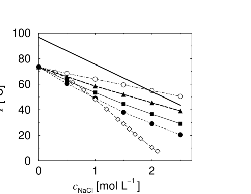
FIG. 4: Predictions of the first-order transition temperatures in the sequential wetting of hexane on brine for various values of the depletion-layer thickness $\delta$; from top to bottom: 2.5 Å (open circles, dash-dotted line), 2.125 Å (filled triangles, thick long-dashed line), 1.9 Å (filled squares, thin continuous line), 1.75 Å (filled circles, thin dashed line), concentration-dependent $\delta$ according to Onsager–Samaras theory [33, 42] (open diamonds, thin long-dashed line). The thick continuous line marks the critical wetting transition temperatures as calculated from the Hamaker constant.

In sharp contrast to this behavior, the first-order transition temperature is rather sensitive to small changes of $\delta$. In Fig. 4, we have compiled the values of $T_{w,1}(c_{\rm NaCl})$ for $\delta=1.75,1.9,2.125$, and 2.5 Å. While these thicknesses are still suitable for describing the surface tension of NaCl solutions (cf. Fig. 3), the predictions of $T_{w,1}$ are not satisfactory, except for $\delta\approx 1.9$ Å. (Note, however, that because of the curvature of $T_{w,1}(c_{\rm NaCl})$, choosing $\delta=1.75$ Å yields good agreement at higher salt concentrations, e.g. for $c_{\rm NaCl}$ = 2.5 mol/L.) In fact, if one chooses $\delta$ large enough, one may even create – purely hypothetically, of course – the elusive critical endpoint, where $T_{w,1}$ coincides with $T_{w,c}$.

For comparison, we also compute $\delta$ from Onsager–Samaras theory as Bertrand et al. did [30, 42]; the prediction of $T_{w,1}(c_{\rm NaCl})$ within our approach (see open diamonds in Fig. 4) shows the same downwards-bend as in their theory. The disagreement of calculated and experimental values of $T_{w,1}$ is therefore mainly due to the inapplicability of Onsager–Samaras theory, which predicts a varying $\delta$ because it neglects the hydration sphere and bases the estimate of $\delta$ solely on electrostatic considerations. Doing so is correct for very low concentrations of salt, but certainly not for the concentrations present in the experiments on sequential wetting. In conclusion, what causes the disagreement is not the breakdown of Debye–Hückel theory, as Bertrand et al. proposed [30], even though this theory is definitely not applicable for the bulk properties of a salt solution in this concentration range. As Levin and Flores-Mena argue [36], the reason why a theory of the surface tension based on Debye–Hückel theory still works for these relatively high salt concentrations is that, in the canonical-ensemble approach introduced by Levin [35], the increase of the interfacial tension is given by the difference between the bulk free energy of a homogeneous system and that of an inhomogeneous system which features the liquid-vapor(air) interface. Therefore, most bulk effects simply cancel.

IV. DISCUSSION AND CONCLUSION

In the preceding sections, we have demonstrated that a DLP-style theory [32] combined with Israelachvili’s approximations [24] and a modern account of the surface tension of electrolytes [36] is able to describe not only the critical-wetting transition temperatures, but also the notoriously more difficult to predict first-order transition temperatures in the sequential-wetting scenario of hexane on brine.

A crucial step in the description of the first-order transition temperature is the determination of the thickness $\delta$ of the depletion layer, a thin film of pure water that forms near the brine/alkane interface. The two attempts made up to now to describe the wetting temperatures in the sequential wetting of hexane on brine rely on a multi-layer (four or five layers, respectively) DLP-type calculation involving layers of brine, water, dense liquid hexane in our case, liquid hexane, and vapor. In the first approach by Bertrand et al. [30, 42], the free energy per unit area of such a four-layer structure is calculated, identified with the shift in contact energy caused by adding the salt, and subsequently converted into a shift of the first-order transition temperature as compared to the first-order wetting transition temperature of hexane on pure water in a conventional Cahn theory using a phase-portrait technique. The values of $T_{w,1}$ resulting from this approach were shown to depend sensitively on the value of $\delta$ [30]. Excellent agreement with the experimental data was found for $\delta\approx 2$ Å.

Similarly, the predictions of $T_{w,1}$ within our approach presented in Sec. II. are in very good agreement with the experimental results if we choose $\delta$ to be approximately 1.9 Å. Interestingly, our theory is as sensitive towards changes in $\delta$ as the one by Bertrand et al. (cf. Fig. 4). Therefore, both treatments have descriptive, but hardly any predictive power. We can conclude that the thickness of the layer of pure water is 1.8 – 2 Å, but we would not be able to predict this thickness to within comparable accuracy for a different salt. In particular, there is a priori no reason why, for a different salt, the graphs of $T_{w,1}(c_{\rm NaCl})$ and $T_{w,c}(c_{\rm NaCl})$ should be parallel; the two lines might actually meet in a critical endpoint. In view of the missing predictive power of the approach, i.e. without knowing $\delta$ beforehand, however, there is no point in calculating the two lines of transition temperatures for another salt at the current state of theory. It is worthwhile noting that the value of 1.8 – 2 Å for the hydrodynamic radius of Na⁺ and Cl^- is consistent with values determined in alternative ways [37] and reasonably well suited for describing the surface tension of NaCl solutions within the theory of Levin and Flores-Mena (cf. Fig. 3).

The major differences between the two approaches presented up to now, by Bertrand et al. and by us, are, firstly, in the way in which the changes due to the addition of salt are attributed to short-range and long-range forces, respectively, and, more importantly, in the reasoning why the depletion-layer thickness $\delta$ should be constant. With respect to the former, our approach is to leave the contact energy (clearly a short-range interaction) unaltered as compared to the case of hexane on pure water since, as before, due to the presence of the depletion layer of thickness $\delta$, only pure water is in direct contact with the adsorbate. We also retain the long-range forces between the layer of pure water and hexane; however, there are new terms in the long-range field which describe the interaction between the brine phase and the adsorbate across the ‘layer’ of pure water of thickness $\delta$. All contributions to the free-energy functional in Eq. (32) are calculated at the actually relevant temperature. Thus, our approach enables us to obtain absolute values of $T_{w,c}$ and $T_{w,1}$ if $\delta$ is determined from independent measurements of the hydrodynamic radius or deduced by matching to the experimental (wetting) transition temperatures.

The second and main difference of our treatment to the one proposed by Bertrand et al. is the justification of having a constant, i.e. salt-concentration independent, depletion-layer thickness $\delta$. Bertrand et al. attribute the existence of this layer to electrostatic image charges that repel the ions from the brine/alkane interface. Based on this mechanism, Onsager and Samaras [33] had developed their theory of the increase of the surface tension of water on the addition of salt. They succeeded in deriving the correct limiting law for low salt concentrations and – as a by-product of their theory – gave an expression that relates the salt concentration to an equivalent depletion-layer thickness $\delta$. The original Onsager–Samaras theory actually calculates the concentration profile and predicts an exponentially rapid approach of the local salt concentration to its bulk value as one moves away from the interface. By integration over this profile, one can compute the deficiency of ions near the interface. This value can, then, on the assumption that there is a layer which is completely devoid of ions (but, according to Onsager and Samaras, this should not be the case), be converted into an equivalent thickness of such a layer. It is this layer thickness that Bertrand et al. identify with $\delta$ in their approach. Within Onsager–Samaras theory, however, this thickness is predicted to decrease slowly (logarithmically) but significantly with increasing salt concentration, so it is clear that the layer thickness cannot remain constant in the approach of Bertrand et al. [30]. It is noteworthy that the equivalent depletion-layer thickness is only a by-product of the Onsager–Samaras theory and that it is not actually used to compute the excess surface tension of the electrolyte [33].

Our approach, in contrast, is based on the recent theory of Levin and Flores-Mena who argue that at higher salt concentrations ($c_{\rm NaCl}>0.15$ mol/L and, therefore, clearly in the range of salinities present in the sequential-wetting experiments) Onsager–Samaras theory neglects the ‘intrinsic’ depletion layer that is formed by the hydration sphere of the ions (at low concentrations, this contribution is negligible because the electrostatic repulsion creates a much thicker layer). In this picture, it becomes much more transparent why $\delta$ is independent of the salt concentration (as long as there are enough water molecules for each ion to have a complete hydration sphere) and about 2 Å in size. The local salt concentration will increase very rapidly to its bulk value in the region beyond the hydration-determined depletion layer thickness because electrostatic shielding is extremely efficient at high salt concentrations.

In conclusion, the theory presented in this article – as well as the one by Bertrand et al. [30] – is able to describe the first-order transition temperature in the sequential wetting of hexane on brine if the thickness of the depletion layer is chosen to be about 1.9 Å. The predictive capacity of both approaches is, unfortunately, much lower. If one had a more precise a priori knowledge of the hydrodynamic radii of the ions, $T_{w,1}$ and $T_{w,c}$ could be predicted for solutions of different salts, which would be a major advantage because the actual experiments are very time-consuming [18]. Such predictions might help identify suitable candidates of solutes for producing a critical endpoint in the wetting phase diagram, which is of particular interest [18, 29, 48].

TABLE I: Representative equations for the dielectric properties of water, brine, liquid hexane, and vapor. In addition to the relative static dielectric permittivity $\varepsilon(0)$ and the refractive index $n$, a characteristic absorption frequency common to all four media of $\nu_{e}=\omega_{e}/(2\pi)=3\times 10^{15}$ s^-1, which is in the UV range, has been used. $T$ denotes the absolute temperature and $c_{\rm NaCl}$ the salt concentration in the brine phase.

medium	relative static dielectric permittivity $\varepsilon(0)$
water[39]	$249.21-0.79069\,{\rm K^{-1}}\,T+0.72997\times 10^{-3}\,{\rm K^{-2}}\,T^{2}$
brine[49]	$\varepsilon_{\rm water}(0)-11\,{\rm L\,mol^{-1}}\,c_{\rm NaCl}$
hexane[50]	$1.890-0.00155\,{\rm K^{-1}}\,(T-293.15\,{\rm K})$
vapor	$\approx 1$
medium	refractive index $n$
water[51]	$1.33436-1.50585\times 10^{-5}\,{\rm K^{-1}}\,(T-273.15\,{\rm K})-1.94586\times 10^{-6}\,{\rm K^{-2}}$
	$\times\,(T-273.15\,{\rm K})^{2}+5.23889\times 10^{-9}\,{\rm K^{-3}}\,(T-273.15\,{\rm K})^{3}$
brine[52]	$n_{\rm water}+0.00918\,{\rm L\,mol^{-1}}\,c_{\rm NaCl}$
hexane[27]	$n_{\rm water}+0.049-0.0004\,{\rm K^{-1}}\,(T-273.15\,{\rm K})$
vapor	$\approx 1$

TABLE II: Representative equations for the coefficients $a_{3}^{\prime}$ and $a_{4}^{\prime}$, which are given by $a_{3}^{\prime}=-W^{\prime}/(6\pi\rho_{l})$ and $a_{4}^{\prime}=B^{\prime}\sigma/(4\pi\rho_{l})$ as calculated from Eqs. (35) and (36), respectively, using the data listed in Table I, for various concentrations of salt. $W^{\prime}$ and $B^{\prime}$ are the quantities actually listed in the table; $W^{\prime}$ is represented in the form $W^{\prime}=a_{W^{\prime}}+b_{W^{\prime}}\,(T-273.15\,{\rm K})+c_{W^{\prime}}\,(T-273.15\,{\rm K})^{2}$, where $T$ is the absolute temperature, and $B^{\prime}$ is simply given by $B^{\prime}=2\,W^{\prime}$.

$c_{\rm NaCl}$ [mol L-1]	$W^{\prime}$ [J]
	$a_{W^{\prime}}$ [J]	$b_{W^{\prime}}$ [J K-1]	$c_{W^{\prime}}$ [J K-2]
0	0	0	0
0.5	$-5.064\times 10^{-22}$	$5.329\times 10^{-25}$	$1.559\times 10^{-27}$
1.0	$-1.012\times 10^{-21}$	$1.069\times 10^{-24}$	$3.207\times 10^{-27}$
1.5	$-1.516\times 10^{-21}$	$1.609\times 10^{-24}$	$4.998\times 10^{-27}$
2.0	$-2.018\times 10^{-21}$	$2.150\times 10^{-24}$	$7.033\times 10^{-27}$
2.5	$-2.519\times 10^{-21}$	$2.689\times 10^{-24}$	$9.509\times 10^{-27}$

FIG. 1: Part (a) shows the geometry of the four-layer structure water(1)/dense liquid hexane(4)/liquid hexane(3)/vapor(2) that is considered for the wetting of hexane on pure water. Part (b) extends this picture for the wetting of hexane on brine and introduces a fifth layer in a structure of the following type: brine(1)/water(4)/dense liquid hexane(5)/liquid hexane(3)/vapor(2). The film thicknesses of the various layers (4, 5, 3) are labeled $\delta$, $\sigma$, and $l$, respectively.

FIG. 3: Excess surface tension of a 1-1 electrolyte, e.g. NaCl, over that of pure water as a function of the salt concentration. The filled circles represent the experimental data for NaCl at 25^∘C obtained by Matubayasi et al.[47] The lines are results of calculations based on the theory of Levin and Flores-Mena [36] using different values for the hydrodynamic radius $\delta$ of the ions; from top to bottom: 2.5 Å (dash-dotted), 2.125 Å (thick long-dashed), 1.9 Å (continuous), 1.75 Å (thin dashed).

References

- [1] J.S. Rowlinson and B. Widom, Molecular Theory of Capillarity (Clarendon, Oxford, 1982).
- [2] J.W. Cahn, J. Chem. Phys. 66, 3667 (1977).
- [3] M.R. Moldover and J.W. Cahn, Science 207, 1073 (1980).
- [4] D. Bonn, H. Kellay, and G.H. Wegdam, Phys. Rev. Lett. 69, 1975 (1992).
- [5] J.E. Rutledge and P. Taborek, Phys. Rev. Lett. 69, 937 (1992).
- [6] E. Cheng, G. Mistura, H.C. Lee, M.H.W. Chan, M.W. Cole, C. Carraro, W.F. Saam, and F. Toigo, Phys. Rev. Lett. 70, 1854 (1993).
- [7] H. Kellay, D. Bonn, and J. Meunier, Phys. Rev. Lett. 71, 2607 (1993).
- [8] H. Nakanishi and M.E. Fisher, Phys. Rev. Lett. 49, 1565 (1982).
- [9] R. Lipowsky and D.M. Kroll, Phys. Rev. Lett. 52, 2303 (1984).
- [10] S. Dietrich and M. Schick, Phys. Rev. B 31, 4718 (1985).
- [11] E. Brézin, B.I. Halperin, and S. Leibler, Phys. Rev. Lett. 50, 1387 (1983).
- [12] R. Lipowsky, Phys. Rev. Lett. 52, 1429 (1984).
- [13] M.P. Nightingale, W.F. Saam, and M. Schick, Phys. Rev. B 30, 3830 (1984).
- [14] D.S. Fisher and D.A. Huse, Phys. Rev. B 32, 247 (1985).
- [15] V.B. Shenoy and W.F. Saam, Phys. Rev. Lett. 75, 4086 (1995).
- [16] D. Ross, D. Bonn, and J. Meunier, Nature (London) 400, 737 (1999), J. Chem. Phys. 114, 2784 (2001).
- [17] K. Ragil, J. Meunier, D. Broseta, J.O. Indekeu, and D. Bonn, Phys. Rev. Lett. 77, 1532 (1996).
- [18] N. Shahidzadeh, D. Bonn, K. Ragil, D. Broseta, and J. Meunier, Phys. Rev. Lett. 80, 3992 (1998).
- [19] P. Richmond, B.W. Ninham, and R.H. Ottewill, J. Colloid Interface Sci. 45, 69 (1973).
- [20] A. Dussaud and M. Vignes-Adler, Langmuir 13, 581 (1997).
- [21] E. Bertrand, H. Dobbs, D. Broseta, J. Indekeu, D. Bonn, and J. Meunier, Phys. Rev. Lett. 85, 1282 (2000).
- [22] K. Ragil, D. Bonn, D. Broseta, and J. Meunier, J. Chem. Phys. 105, 5160 (1996).
- [23] H. Dobbs, J. Chem. Phys. 114, 468 (2001).
- [24] J.N. Israelachvili, Intermolecular and Surface Forces (Academic Press, London, 1985).
- [25] J.O. Indekeu, K. Ragil, D. Bonn, D. Broseta, and J. Meunier, J. Stat. Phys. 95, 1009 (1999).
- [26] V.C. Weiss and B. Widom, Physica A 292, 137 (2001).
- [27] K. Ragil, Ph.D. thesis, Université Pierre et Marie Curie – Paris VI (1996).
- [28] R. Aveyard and S.M. Saleem, J. Chem. Soc. Faraday Trans. 72, 1609 (1976).
- [29] V.C. Weiss and J.O. Indekeu, Physica A 301, 37 (2001).
- [30] E. Bertrand, D. Bonn, and J. Meunier, Phys. Rev. Lett. (Reply) 85, 4189 (2000).
- [31] J.O. Indekeu, Phys. Rev. Lett. (Comment) 85, 4188 (2000).
- [32] I.E. Dzyaloshinskii, E.M. Lifshitz, and L.P. Pitaevskii, Adv. Phys. 10, 165 (1961).
- [33] L. Onsager and N.N.T. Samaras, J. Chem. Phys. 2, 528 (1934).
- [34] R. Massoudi and A.D. King, Jr., J. Phys. Chem. 79, 1670 (1975).
- [35] Y. Levin, J. Chem. Phys. 113, 9722 (2000).
- [36] Y. Levin and J.E. Flores-Mena, Europhys. Lett. 56, 187 (2001).
- [37] B.E. Conway, Electrochemical Data (Elsevier, Amsterdam, 1952).
- [38] D.Y. Peng and D.B. Robinson, Ind. Eng. Chem. Fund. 15, 59 (1976).
- [39] D.R. Lide (ed.), CRC Handbook of Chemistry and Physics, 73rd ed. (CRC Press, Boca Raton, FL, 1992-93).
- [40] R.C. Reid, J.M. Prausnitz, and T.K. Sherwood, The Properties of Gases and Liquids, 3rd ed. (McGraw-Hill, New York, NY, 1977).
- [41] B.S. Carey, L.E. Scriven, and H.T. Davis, AIChE J. 24, 1076 (1978).
- [42] E. Bertrand, Ph.D. thesis, Université Pierre et Marie Curie – Paris VI (2000).
- [43] E. Bertrand, D. Bonn, H. Kellay, B.P. Binks, and J. Meunier, Europhys. Lett. 55, 827 (2001).
- [44] J. Mahanty and B.W. Ninham, Dispersion Forces (Academic Press, London, 1976).
- [45] V.A. Parsegian and B.W. Ninham, J. theoret. Biol. 38, 101 (1972).
- [46] H. Sagan, Introduction to the Calculus of Variations (McGraw–Hill, New York, NY, 1969).
- [47] N. Matubayasi, H. Matsuo, K. Yamamoto, S. Yamaguchi, and A. Matuzawa, J. Colloid Interface Sci. 209, 398 (1998).
- [48] D. Bonn, E. Bertrand, N. Shahidzadeh, K. Ragil, H.T. Dobbs, A.I. Posazhennikova, D. Broseta, J. Meunier, and J.O. Indekeu, J. Phys.: Condens. Matter 13, 4903 (2001).
- [49] J.B. Hasted, D.M. Ritson, and C.H. Collie, J. Chem. Phys. 16, 1 (1948).
- [50] R.C. Weast (ed.), CRC Handbook of Chemistry and Physics, 66th ed. (CRC Press, Boca Raton, FL, 1985-86), as cited by Ragil[27].
- [51] Fit to data taken from Lide[39].
- [52] Generalization of representative equations for the refractive index of brine for various salt concentrations given by Shahidzadeh et al. [18] and by Ragil[27].