Localization of Denaturation Bubbles in Random DNA Sequences

Abstract

We study the thermodynamic and dynamic behaviors of twist-induced denaturation bubbles in a long, stretched random sequence of DNA. The small bubbles associated with weak twist are delocalized. Above a threshold torque, the bubbles of several tens of bases or larger become preferentially localized to AT-rich segments. In the localized regime, the bubbles exhibit “aging” and move around sub-diffusively with continuously varying dynamic exponents. These properties are derived using results of large-deviation theory together with scaling arguments, and are verified by Monte-Carlo simulations.

I Introduction

Localized opening of double-stranded DNA is essential in a number of cellular processes such as the initiations of gene transcription and DNA replication Alberts . While thermal denaturation is highly unlikely under physiological conditions, in vitro experiments show that local denaturation can be readily induced by under-winding the DNA double helix by an amount that is physiologically reasonable Kowalski , Cozzarelli , Bensimon . The basic physical effect is simple: An under-wound double helix suffers a reduction in the binding free energy Marko , Cocco , Strick00 . Local openings of the double helix (referred to as “denaturation bubbles”) relieve the twist experienced by the remainder of the double helix and is thus energetically favorable. The denaturation bubbles may be recruited to a specific location of the genome by a designed (e.g., AT-rich) sequence, since AT pairs bind more weakly than GC pairs Benham . On the other hand, entropic effect which favors bubble delocalization is non-negligible for long sequences. Also significant is the kinetic trapping of the bubbles due to statistical agglomeration of AT-rich segments in long heterogenous sequences.

To gain some quantitative understanding on the competing effects of entropy and sequence heterogeneity, we characterize in this study the thermodynamic and dynamic properties of denaturation bubbles in a long, stretched random DNA sequence with no special sequence design. Previously, there have been a number of experimental and theoretical studies Cule , tang01 , Heslot , Lubensky on the effect of sequence heterogeneity on DNA melting and unzipping transitions. Our study is along this general direction. The specific behaviors exhibited by the denaturation bubbles are rather complex and are typical of those observed in systems dominated by quenched disorders glass : The bubbles are localized upon increase of the applied torque beyond a certain threshold. In the localized regime, their dynamics exhibits “aging” aging1 , aging and is sub-diffusive with continuously varying exponents.

Interestingly, twist-induced denaturation presents a rare physical example of the celebrated random-energy model of disordered system rem . Consequently, detailed analysis of both the thermodynamis and dynamic properties can be made by applying the well-developed theory of disordered systems glass , together with exact results from large-deviation theory familiar in the related sequence alignment problem KarlinAltschul , YuHwa . We will draw upon detailed experimental knowledge of thermal denaturation SantaLucia , SantaLucia1 , Blake throughout the analysis, and make our results quantitative whenever possible.

II Thermodynamics

Let us consider the application of a torque which under-winds a long, stretched piece of double-stranded DNA. We are interested in the regime where the applied torque ${\cal T}$ is below the threshold ${\cal T}_{\rm d}$ for bulk denaturation, but sufficiently strong so that denaturation bubbles do appear in the system. Due to the highly cooperative nature of the denaturation process, the typical distance $N_{\times}$ between the large bubbles is large, in which case treating the bubbles as a dilute gas of particles is appropriate. Our strategy will be to first characterize analytically the thermodynamic behavior of a single bubble, and then use this knowledge to determine the length scale $N_{\times}$ and the many-bubble states for $N\gg N_{\times}$. We will find that $N_{\times}>O(10^{3})\,{\tt bp}$ as long as we are not very close to the threshold ${\cal T}_{\rm d}$, so that the dilute gas approximation is reasonable for a large range of parameters.

II.1 The Single-bubble Model

Consider a denaturation bubble confined in a DNA double helix between two complementary DNA strands of $N$ bases each. The double-strand is denoted by the base sequence $b_{1}b_{2}\ldots b_{N}$ [with $b_{k}\in\{{\tt A,C,G,T}\}$] of one of the strands, ordered from the 5’- to 3’- end. To simplify the notation, we assume that the two ends of the helix is sealed, so that the bubble is always contained in the segment $b_{1}\ldots b_{N}$. Let the index of the first and last open pairs of the open bubble be $m$ and $n$, with $1\leq m\leq n\leq N$. We denote the total free energy of the bubble (defined with respect to the helical state) by $\Delta G_{L}(m)$, where $L\equiv n-m+1$ is the number of open bases and referred to as the bubble length. Then the partition function of the single-bubble system is given by

$$Z(N)=\sum_{L=1}^{N}\sum_{m=1}^{N-L+1}e^{-\beta\Delta G_{L}(m)}\;,$$ (1)

where $\beta^{-1}\equiv k_{B}T\simeq 0.62~{}{\tt kcal/mole}$ at $37^{\circ}{\tt C}$.

In the absence of the external torque, the bubble energy $\Delta G_{L}(m)$ has two components. First, there is the loss of stacking energy $\delta G_{b,b^{\prime}}$ between two successive bases $b$ and $b^{\prime}$. These stacking energies are in the range $0.5\sim 2.5\,k_{B}T$’s at $37^{\circ}{\tt C}$, with the AT stacks weaker than the GC stacks. Their values have been measured carefully SantaLucia , SantaLucia1 , Blake . Second, assuming that there is no secondary pairing between bases in the bubble so that the open configuration can be regarded as a polymer loop, there is a well-known polymeric loop entropy cost

$$\gamma_{L}=\gamma_{1}+\alpha\cdot k_{B}T\;\ln L$$ (2)

for a bubble of length $L$, with $\alpha\approx 1.8$ MEFisher for a linearly extended DNA chain. The bubble initiation cost $\gamma_{1}$ depends on the base composition at opening and closing ends, ionic strength etc., and generally lies in the range $3\sim 5\,k_{B}T$. For relevant bubble sizes of few tens of bases in length (see below), the total entropic cost is $\gamma_{L}=8\sim 12\,k_{B}T$. This large cost justifies the single bubble approximation (at least to the length scale $N_{\times}\sim e^{\beta\gamma_{L}}\gtrsim 5\times 10^{3}\,{\tt bp}$), and contributes significantly to the sharpness of the observed thermal denaturation transition Blake .

An applied negative torque ${\cal T}$ reduces the thermodynamic stability of the helical state relative to the denatured one by an amount equal to the work done to unwind the helix. This effect is simply modeled here by a linear decrease in the stacking energy in the relevant parameter range Cocco , i.e., $\delta G_{b,b^{\prime}}\to\delta G_{b,b^{\prime}}-\theta_{0}\,{\cal T}$, where $\theta_{0}=2\pi/10.35$ is the twist angle per base of the double helix. Putting the above together, we have

$$\Delta G_{L}(m)=\gamma_{L}+\sum_{k=m}^{m+L}\delta G_{b_{k-1},b_{k}}-\theta_{0}\,{\cal T}\cdot L$$ (3)

as the single bubble energy, which can be computed once the DNA sequence $b_{1}...b_{N}$ is given. Note that while Eq. (3) is formulated specifically for twist-induced denaturation, the general form can be used to describe a number of destabilizing effects, e.g., due to changes in temperature, ionic concentration, etc.

II.2 Sequence Heterogeneity

As the torque ${\cal T}$ increases from zero towards the denaturation point ${\cal T}_{\rm d}$, denaturation bubbles appear in the double strand and grow in size. We wish to know whether the bubbles are free to diffuse along the double strand, or are they localized in the high AT regions of the DNA where binding is the weakest. For simplicity, we will characterize the typical behavior of an ensemble of random (i.e., independent and identically distributed) sequences described by the single-nucleotide frequencies $p_{b}$, although our approach and qualitative findings are also applicable to sequences with short-range correlations.

For a given sequence of bases, the partition function $Z$ can of course be efficiently evaluated numerically (including all the multiple-bubble states) by using available programs such as MELTSIM Blake . All thermodynamic quantities can subsequently be evaluated from the free energy $F=-k_{B}T\ln Z$. To obtain the typical behavior of the ensemble, we ideally want to compute the ensemble average of the free energy, $\overline{F}\equiv-k_{B}T\,\overline{\ln Z}$. [We use the over-line to denote average over the ensemble of random sequences, i.e., $\overline{X}\equiv\sum_{b_{1},...,b_{N}}X_{b_{1},...,b_{N}}\prod_{k=1}^{N}p_{b_{k}}$; this is also known as the “disorder average”.] Computing $\overline{F}$ numerically however will require explicit generation of a large number of random sequences and can be very time consuming for large $N$’s. Fortunately we can apply a large body of knowledge accumulated from the statistical mechanics of random systems glass and provide a detailed characterization of the typical behavior of our system without the need of exhaustive simulation. To introduce notation and concepts in this approach, we examine first the simplified problem of a single bubble with a fixed length.

II.3 Bubble with Fixed Length

Let us consider a bubble with a fixed length $L$ (with $1\ll L\ll N$) embedded in a long, random sequence $b_{1}...b_{N}$. The partition function reads

$${\cal Z}_{L}=\sum_{m=1}^{N-L+1}\exp[-\beta\Delta G_{L}(m)],$$ (4)

where the scripted variables refer to properties of the fixed length bubble. For a random sequence, the energies of the different states labeled by $m$ are uncorrelated with each other beyond the distance $L$. Such systems belong to the class of “Random Energy Model” (REM) and was solved exactly in the 80’s by Derrida rem for a Gaussian distribution of $\Delta G$’s. Discrete distribution of $\Delta G$’s was studied in the closely-related system involving protein-DNA interaction Gerland . Below, we will briefly review the salient properties of REM using the present example.

The REM has a “high-temperature” phase where many (of order $N$) bubble configurations contribute significantly to the partition sum, and a “low-temperature” phase dominated by only one or a few lowest energy states. It follows that, in the former case, the bubble is delocalized and can freely diffuse along the sequence, while in the latter case, the bubble is localized to the lowest energy position. Transition between the two phases is driven by competition between the energetic (variation in $\Delta G$) and entropic ($\ln N$) effects. In the present problem, the magnitude of terms in the partition sum (4) can be tuned not only by varying the temperature, but also by varying the bubble size $L$. Hence, at a fixed $\beta$, whether a bubble is free or localized depends both on the bubble size $L$ and the sequence length $N$.

An interesting property of the REM is that, in the “high-temperature” phase, ${\cal Z}_{L}/N$ tends to a finite limit given by the annealed average $\overline{{\cal Z}}_{L}/N$ as $N\rightarrow\infty$, independent of the particular realization of the random sequence. This allows us to replace the average free energy $\overline{{\cal F}}\equiv-k_{B}T\,\overline{\ln{\cal Z}}$ by its annealed approximation $\widetilde{{\cal F}}\equiv-k_{B}T\ln\overline{{\cal Z}}$, which is much easier to calculate. [We will use the tilde to denote all quantities computed in the annealed approximation.] Introducing a $4\times 4$ matrix $\mbox{\boldmath$\mathsf{M}$}(\beta)$ with components $\mathsf{M}_{b,b^{\prime}}=\sqrt{p_{b}p_{b^{\prime}}}\exp[-\beta\;\delta G_{b,b^{\prime}}]$, and let the largest eigenvalue of $\mbox{\boldmath$\mathsf{M}$}(\beta)$ be $\Lambda(\beta)$, then the disorder average of terms in (4) can be written as

$$\overline{e^{-\beta\sum_{k=m}^{m+L-1}\delta G_{b_{k-1},b_{k}}}}={\rm Tr}\ \mbox{\boldmath$\mathsf{M}$}^{L}(\beta)\stackrel{{\scriptstyle L\gg 1}}{{=}}\Lambda^{L}(\beta).$$ (5)

It is convenient to introduce the quantity

$$f(\beta)\equiv-\beta^{-1}\ln\Lambda(\beta),$$ (6)

with which we have (for $N\gg L$)

$$\overline{{\cal Z}}_{L}=\frac{N\,e^{-\beta\gamma_{1}}}{L^{\alpha}}\,\left[e^{-\beta[f(\beta)-\theta_{0}{\cal T}]}\right]^{L}.$$ (7)

Hence, in the delocalized phase, $\overline{{\cal F}}\simeq\widetilde{{\cal F}}=-k_{B}T\ln N+L[f(\beta)-\theta_{0}{\cal T}]+\gamma_{L}$.

The annealed entropy can be calculated from $\widetilde{{\cal F}}$, with

$$\widetilde{{\cal S}}=-k_{B}^{-1}{\partial\widetilde{{\cal F}}\over\partial T}=\ln N-\beta[f(\beta)-\varepsilon(\beta)]L,$$ (8)

where $\varepsilon(\beta)\equiv-\frac{\partial}{\partial\beta}\ln\Lambda.$ It will also be useful to introduce the relative entropy per base for the fixed-length bubble,

$${\cal H}(\beta)\equiv[\ln N-\widetilde{{\cal S}}]/L=\beta[f(\beta)-\varepsilon(\beta)].$$ (9)

Note that being the difference between $f$ and $\varepsilon$, the quantity ${\cal H}$ is a measure of the intrinsic variation in the binding energies $\delta G$’s for a random sequence with nucleotide frequency $p_{b}$, and is independent of the average binding energy $\overline{\delta G}$ which external environment such as the temperature or solvent conditions most directly affect.

Derrida’s solution of REM shows that the annealed entropy $\widetilde{{\cal S}}$ vanishes at the transition to the “low-temperature” phase, beyond which the annealed approximation is no longer applicable. Using Eqs. (8) and (9), we can write the condition for phase transition as

$$L_{\rm loc}=\ln N/{\cal H}(\beta),$$ (10)

which gives the minimal bubble size for localization at a given $N$. With the values of $\delta G$’s obtained from Ref. SantaLucia at $[{\rm Na}^{+}]=1~{}{\tt M}$ and $37^{\circ}{\tt C}$, and assuming an equal nucleotide distribution (i.e., $p_{b}=1/4$ for all bases), we find $f\approx 1.83\,k_{B}T$, $\varepsilon\approx 1.50\,k_{B}T$, so that ${\cal H}\approx 0.33$ and $L_{\rm loc}\approx 20\,{\tt bp}$ for $N\sim 10^{3}\,{\tt bp}$. From Eq. (10), it is clear that as $N\to\infty$ any fixed-length bubble remains delocalized.

II.4 Bubble without Length Constraint

The full partition function $Z$ is obtained simply by summing ${\cal Z}_{L}$ for different $L$’s. We will again approach the problem by first applying the annealed approximation and then determining where it breaks down.

1. Annealed approximation: The annealed partition function $\overline{Z}(N)\equiv\sum_{L=1}^{N}\overline{{\cal Z}}_{L}$ has a transition at ${\cal T}_{\rm a}=f(\beta)/\theta_{0}$, where the exponential factor in (7) reaches one: The sum over $L$ is finite and $\overline{Z}\propto N$ only if ${\cal T}<{\cal T}_{\rm a}$. In this regime, the annealed free energy is simply $\widetilde{F}\approx-k_{B}T\ln N+\gamma_{1}.$ The annealed energy $\widetilde{E}\equiv-\frac{\partial}{\partial\beta}\ln\overline{Z}(\beta)$ is also readily computed; it can be expressed as $\widetilde{E}=\gamma_{1}+[\varepsilon(\beta)-\theta_{0}{\cal T}]\cdot\widetilde{L}$ where $\widetilde{L}({\cal T})\equiv\sum_{L=1}^{N\to\infty}L\,\overline{{\cal Z}}_{L}/\overline{Z}$ is the average bubble length in the annealed approximation. As ${\cal T}$ approaches ${\cal T}_{\rm a}$, $\widetilde{L}({\cal T})$ diverges, and the annealed entropy

$$\widetilde{S}=\ln N-\beta[\theta_{0}{\cal T}-\varepsilon(\beta)]\cdot\widetilde{L}$$ (11)

becomes negative.

In the limit $N\to\infty$, the anealed free energy $\widetilde{F}$ is actually identical to $\overline{F}$ for all ${\cal T}\leq{\cal T}_{\rm a}$. This can be seen from the inequalities $\overline{\ln{\cal Z}_{L=1}}\leq\overline{\ln Z}\leq\ln\overline{Z},$ and ${\cal Z}_{L=1}>N\min\{\exp[-\beta\Delta G_{1}]\}$. Since both the lower and upper bounds grow as $\ln N$,

$$\overline{F}\equiv-k_{B}T\overline{\ln Z}\simeq-k_{B}T\ln N$$ (12)

for all ${\cal T}\leq{\cal T}_{\rm a}$.

2. Ground-state properties: To find the ground-state of the unconstrained bubble in a long random sequence, we need to study the statistics of stretches of exceptionally high AT-content. If we neglect the polymeric contribution $\gamma_{L}$ to the bubble energy [to be justified shortly], then the ground-state energy $E^{*}$ expected in a sequence of length $N$ can be computed exactly from large-deviation theory KarlinAltschul , Dembo , with

$$\overline{E^{*}}(N)\approx-\lambda^{-1}\ln N.$$ (13)

The constant $\lambda$ in Eq. (13) can be expressed as the unique positive root of the equation

$$f(\lambda)=\theta_{0}{\cal T},$$ (14)

where $f$ is defined by the $\delta G$’s through Eqs. (5) and (6). Note that, at ${\cal T}={\cal T}_{\rm a}$, Eq. (14) is satisfied with $\lambda=\beta$. In this case, (13) coincides with (12).

The length of the minimal energy bubble is also known from large-deviation theory Dembo , YuHwa , with

$$L^{*}({\cal T})=\ln N/H^{*}({\cal T}),$$ (15)

where the relative entropy $H^{*}$ is given exactly by

$$H^{*}({\cal T})=\lambda({\cal T})\cdot[\theta_{0}{\cal T}-\varepsilon(\lambda)].$$ (16)

From the logarithmic dependence of the bubble length $L^{*}$ on $N$, it is clear that the corresponding polymeric contribution $\gamma_{L^{*}}\sim\ln(\ln N)$ can indeed be treated as a constant shift of bubble energy.

3. Phase transitions: Based on the above discussion, a phase transition can be formally established in the limit $N\rightarrow\infty$. This is seen by comparing the expressions (12) and (13). For ${\cal T}>{\cal T}_{\rm a}$, solution to (14) satisfies $\lambda<\beta$. Consequently, (12) must break down there, yielding a phase transition at ${\cal T}={\cal T}_{\rm a}$. Since $\overline{F}\leq\overline{E^{*}}$ in general (e.g., for all ${\cal T}>{\cal T}_{\rm a}$), and at the phase transition point ${\cal T}={\cal T}_{\rm a}$ the equality $\overline{F}=\overline{E^{*}}$ already holds, i.e., the ground-state already dominates, then we must have the ground-state dominating throughout the localized phase. This is exactly the behavior of the random energy model rem .

A physical understanding of the transition can be obtained by examining the importance of the ground-state contribution $\exp(-\beta E^{*})\sim N^{\beta/\lambda}$ to the partition sum $Z$ as the applied twist ${\cal T}$ is varied. For ${\cal T}<{\cal T}_{\rm a}$, the ratio $\beta/\lambda({\cal T})$ is less than one. In this case, the energy gain $\overline{E^{*}}(N)$ of placing the bubble at the site of the lowest energy is insufficient to overcome the entropy $\ln N$ of placing the bubble in different positions, hence the bubble is typically small and delocalized. When ${\cal T}$ exceeds ${\cal T}_{\rm a}$, the ground-state contribution grows faster than $N$, signalling dominance of one or a few low energy states where the bubble typically resides. The transition is thus identified as the localization transition of the bubble at ${\cal T}_{\rm loc}={\cal T}_{\rm a}$.

The onset of the zero entropy point can be obtained from Eq. (11) and written as

$$\ln N={H}(\beta,{\cal T})\cdot\widetilde{L}(\beta,{\cal T}),$$ (17)

where

$${H}(\beta,{\cal T})=\beta\cdot[\theta_{0}{\cal T}-\varepsilon(\beta)]$$ (18)

is the relative entropy of the unconstrained bubble. These equations are analogous to the expressions (15) and (16) for the ground-state bubble. In fact, both $L^{*}({\cal T})$ and $H^{*}({\cal T})$ are reproduced through the substitution $\beta\rightarrow\lambda({\cal T})$, e.g., $L^{*}({\cal T})=\widetilde{L}(\lambda({\cal T}),{\cal T})$. This turns out to be true also for other thermodynamic variables. Thus the localized phase at different ${\cal T}$’s can be viewed as the phase transition points of systems with different effective temperatures $\lambda^{-1}({\cal T})$; this will be clearly manifested in the bubble dynamics discussed below.

Next we observe that since $H^{*}\propto\lambda$ [see Eq. (16)], the bubble length diverges (or approaches $N$) as $\lambda\to 0$. This defines the point of bulk denaturation ${\cal T}_{\rm d}$, i.e.,

$$\theta_{0}{\cal T}_{\rm d}\equiv\lim_{\lambda\to 0}f(\lambda)=\overline{\delta G},$$ (19)

where the second equality is obtained from manipulating Eqs. (5) and (6). Using $\overline{\delta G}\approx 1.40\ k_{B}T$ [derived from the $\delta G$’s in Ref. SantaLucia ], we find ${\cal T}_{\rm d}\approx 10\ {\rm pN}\cdot{\rm nm}$. The dependence of $\lambda$ on ${\cal T}$ close to ${\cal T}_{\rm d}$ can be obtained from the expansion

$$f(\lambda)=\overline{\delta G}-\frac{\lambda}{2}{\rm var}(\delta G)+O(\lambda^{2}).$$ (20)

Inverting the above for $\lambda$ using (14) and (19), we find

$$\lambda({\cal T})=\frac{2\theta_{0}}{\beta{\rm var}(\delta G)}\ \big{(}{\cal T}_{\rm d}-{\cal T}\big{)}+O\big{(}{\cal T}_{\rm d}-{\cal T}\big{)}^{2}.$$ (21)

It turns out that the term linear in ${\cal T}_{\rm d}-{\cal T}$ in (21) already gives a very good approximation (to within $1\%$) of $\lambda$ throughout the localized phase where $\lambda/\beta<1$. The localization transition point ${\cal T}_{\rm loc}$ can be thus obtained by solving Eq. (21) with $\lambda({\cal T}_{\rm loc})=\beta$. Using $\beta^{2}{\rm var}(\delta G)\approx 0.565$ [derived from Ref. SantaLucia ], we find ${\cal T}_{\rm d}-{\cal T}_{\rm loc}\approx 2\ {\rm pN}\cdot{\rm nm}$. Unlike the value of ${\cal T}_{\rm d}$ which is derived from the average stacking energy $\overline{\delta G}$ and hence sensitive to temperature, ionic strength, etc., the difference ${\cal T}_{\rm d}-{\cal T}_{\rm loc}$ is set by the variance of $\delta G_{b,b^{\prime}}$ and should be much less sensitive to experimental conditions. The same is expected for the relative entropy, which has the form

$$H^{*}({\cal T})\approx 2\theta_{0}^{2}({\cal T}_{\rm d}-{\cal T})^{2}/{\rm var}(\delta G)$$ (22)

throughout the localized phase.

II.5 Multiple bubbles

The localization transition discussed above occurs only as $N\to\infty$. However for large $N$, the single-bubble approximation will break down regardless of the large (but finite) bubble cost $\gamma_{L}$. When multiple bubbles are localized, each bubble is effectively in a finite-length system, thereby blurring the localization transition.

We first analyze the delocalized phase for which the annealed approximation is valid. Once multiple bubbles are allowed in the system, we expect a broad range of bubble lengths, as described by the distribution (7). Qualitatively, we expect only the largest bubbles, of size $\widetilde{L}({\cal T})$ to be localized as ${\cal T}\to{\cal T}_{\rm loc}$, while the smaller ones remain delocalized. We shall thus focus on these large bubbles: It is the average separation distance $N_{\times}$ between these large bubbles that sets the effective system size of the single-bubble localization problem.

The Boltzmann weight of one such large bubble in a sequence of length $N\gg\widetilde{L}$ is $\widetilde{W}(N)=e^{-\beta\gamma_{1}}N/\widetilde{L}^{\alpha}$ in the vicinity of the localization transition. Setting $\widetilde{W}(N)=1$ yields the typical spacing between the large bubbles on the delocalized side,

$$\widetilde{N}_{\times}\approx e^{\beta\gamma_{1}}\,\widetilde{L}^{\alpha}({\cal T}).$$ (23)

Note that for bubbles of size $10\,{\tt bp}$’s, the crossover length is already of the order of $10^{3}\,{\tt bp}$’s. A similar estimate can be made on the localized phase using the exact expression KA93 for the lowest energy for multiple bubbles. We find

$$N^{*}_{\times}\approx\bigg{[}e^{\beta\gamma_{1}}\,(L^{*})^{\alpha}\bigg{]}^{\lambda({\cal T})/\beta}.$$ (24)

as the average distance between large bubbles of size $L^{*}$.

For $N\gg N_{\times}$, the system consists of $N/N_{\times}$ effective number of single-bubble subsystems, each of length $N_{\times}$. At the localization “transition” of an infinite system then, we have $\ln\widetilde{N}_{\times}={H}(\beta,{\cal T}_{\rm loc})\widetilde{L}({\cal T}_{\rm loc})$ [see Eq. (17)]. Together with Eq. (23) [or (24) with $\lambda=\beta$], we find $\widetilde{L}({\cal T}_{\rm loc})\approx 25\,{\tt bp}$ at the onset of localization (using $\gamma_{1}\approx 3\,k_{B}T$ and ${H}\approx 0.33$), with the crossover length $\widetilde{N}_{\times}\approx 6500\,{\tt bp}$. Thus we expect there to be typically one bubble of $\sim 25{\tt bp}$ in a random DNA double-strand of length $\sim 6500\,{\tt bp}$’s at the localization transtion.

III Bubble Dynamics

The localization of bubbles is reflected ultimately in their slow dynamics. We expect bubbles to diffuse freely along the DNA double-helix in the delocalized phase, but become trapped in low energy positions in the localized phase. Details of the bubble movement in the latter case, however, can be rather complicated with nontrivial memory (or “aging”) effects typical of glassy states aging1 , aging as will be described below.

III.1 Model

For simplicity, we will restrict ourselves to the description of the movement of a single-bubble over its lifetime, which can be rather long in the localized phase. For reasons discussed above, interaction with other bubbles can be neglected when the bubble displacement is within a distance of order $N_{\times}\sim 10^{3}\,{\tt bp}$. We will also neglect the polymeric loop entropy $\gamma_{L}$ which provides essentially a constant shift to the bubble energy as shown in the single bubble section.

In addition to the drift and breathing motion, a bubble may also shrink to zero size and disappear from the system. To our knowledge, the time scale involved for the spontaneous collapse of a bubble, particularly under an applied twist, has not been documented so far. Zipping the bubble requires not only pairing of the bases in the open segment, but also rewinding of the helix against the applied undertwist, both of which contribute to the energy barrier to the no-bubble state. This suggests a long lifetime for a bubble, which can be enforced by setting a lower bound (e.g., $10\,{\tt bp}$) in the allowed bubble length. However, as we will see, the long-time behavior of bubble dynamics is determined crucially by the occurrence of the large bubble states, and insensitive to the value of the lower bound on $L$, as long as the $L=0$ state is excluded. Once accurate estimates of bubble lifetime become available, one may supplement the discussion below with such a cutoff.

III.2 Scaling Theory

Equation (13) gives the lowest energy of an unconstrained bubble in a sequence of length $N$, while a bubble with its position (but not size) fixed typically has an energy of the order $\lambda^{-1}$ for ${\cal T}<{\cal T}_{\rm loc}$. For small $\lambda$, the energy variation $\Delta E(N)\simeq\lambda^{-1}\ln N$ is large, hence the bubble dynamics is dominated by the thermal escape from the deepest trap. The escape time is thus $t_{\rm e}(N)\simeq e^{\beta\Delta E(N)}\sim N^{\beta/\lambda}$, i.e., the dynamics is sub-diffusive deep in the localized phase (where $\beta\gg\lambda$).

To investigate the dynamical behavior in more detail, especially close to the localization transition where $\lambda\approx\beta$, we need to include also the random motion of the bubble along the double strand. Towards this end, it is useful to describe the bubble dynamics as a single point moving in the two-dimensional space spanned by the bubble’s only two degrees of freedom, its instantaneous length $L$ and the position of one of its ends, say $m$. The statistics of the two-dimensional energy landscape $\Delta G_{L}(m)$ is well-characterized by the large-deviation theory YuHwa . It consists of a number of valleys, whose depths (denoted by $\Delta\widehat{G}$’s) are given by the Poisson distribution

$${\cal D}\left(\left|\Delta\widehat{G}\right|\right)\propto e^{-\lambda\left|\Delta\widehat{G}\right|},$$ (25)

where $\lambda$ is the constant defined through (14). The typical valley length is $\widehat{L}\sim 1/H^{*}$, where $H^{*}$ is given by (16). The valleys are spread out along the corridor at $L\lesssim\widehat{L}$, separated by a typical distance $M$ which is also calculable from the large-deviation theory. For much larger $L$’s, the bubble energy becomes prohibitively high.

Clearly, the dynamics consists of two parts: At short times, it is dominated by the escape of the bubble out of an individual valley, and is analogous to the (biased) Sinai problem Sinai . At longer time scales, the bubble “hops” from one valley to another along the corridor of valleys. This dynamics, which is essentially that of a particle traversing a series of exponentially-distributed energy valleys [see Eq. (25)], has been extensively investigated previously in the context of the one-dimensional “trap” model slowa , slowb . Here we review some key results and refer the readers to Ref. berbou for details. The basic quantity is the time $\tau(\Delta\widehat{G})\propto e^{\beta\left|\Delta\widehat{G}\right|}$ to escape each valley of depth $\Delta\widehat{G}$. The average time to traverse $K$ valleys over a length scale $N=K\cdot M$ by random walk is then given by

$$t_{\rm e}=K^{2}\cdot\langle\tau\rangle\sim N^{2}\int_{\lambda^{-1}}^{|\overline{E^{*}}|}dx\,\tau(x)\,{\cal D}(x),$$ (26)

where $\langle\tau\rangle$ is the average of the trap time $\tau(\Delta\widehat{G})$, and the limits of integration in (26) are from the magnitude of the typical valley depth $\lambda^{-1}$ to that of the deepest valley (13) expected for a segment of length $N$.

The total time according to Eq. (26) can be written as $t_{\rm e}(N)\propto N^{z}$, with the dynamic exponent $z$ given by

$$z=\left\{\begin{tabular}[]{ll}$2$&\quad for ~{} $\lambda>\beta$ ~{} (or ${\cal T}<{\cal T}_{\rm loc}$)\\ $1+\beta/\lambda$&\quad for ~{} $\lambda<\beta$ ~{} (or ${\cal T}_{\rm loc}<{\cal T}<{\cal T}_{\rm d}$)\end{tabular}\right.$$ (27)

The anomalous exponent $z>2$ in the glass phase shows explicitly that the dynamics is slow, i.e., sub-diffusive.

III.3 Glassy Dynamics

We next report the result of a Monte-Carlo simulation of the bubble dynamics on predefined random nucleotide sequences. We impose local dynamics in which the bubble can only change its length $L$ or shift its end position $m$ by a single base, as long as $L\geq 1$. To remove edge effects and probe the asymptotic dynamics, we use a very large sequence length ($>10^{4}\ {\tt bp}$) so that the bubble never reaches the boundary of the sequence given the duration of our numerical study. All disorder-averaged quantities reported are performed over $10^{4}$ random sequences.

1. Anomalous diffusion: To characterize the slow dynamics quantitatively, we show in Fig. 1(a) the time evolution of the average displacement $R(t)=|m(t)-m(0)|$ of the bubble position for a few selected values of ${\cal T}$’s in the glass phase. Clearly, the displacement can be described by a power law of the form $R(t)\propto t^{\nu}$, where we expect $\nu=1/z$. In Fig. 1(b), we plot the extracted exponents (circles) for different values of ${\cal T}$’s in the range ${\cal T}_{\rm loc}\leq{\cal T}<{\cal T}_{\rm d}$. The expected values $1/z$ according to Eq. (27) (using the linear expression in (21) for $\lambda$) is shown as the solid line for comparison. We note that the observed exponents follow the general trend predicted, changing continuously from $1/z=0.5$ close to the expected location of the glass transition (${\cal T}_{\rm loc}\approx 0.8{\cal T}_{\rm d}$), towards zero as ${\cal T}\to{\cal T}_{\rm d}$. For ${\cal T}$ close to ${\cal T}_{\rm d}$, the dynamics becomes exceedingly slow, making it difficult to access the asymptotic region. For ${\cal T}\approx{\cal T}_{\rm loc}$, we also observed some finite-size effect. The overall agreement between the scaling theory and numerical results is within $5\sim 10\%$ over the range tested.

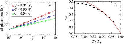
Figure 1: (a) Average bubble position vs time for various values of ${\cal T}$’s in the glass phase: the solid lines are power law fits. (b) The extracted exponents vs ${\cal T}$: the solid line is the prediction of the scaling theory Eq. (27).

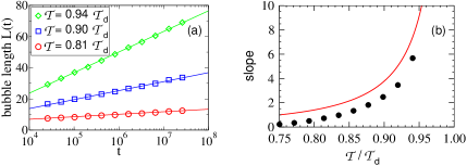
Figure 2: (a) Average bubble length vs time for several ${\cal T}$’s; the solid lines are fits to the form $L(t)=a+b\,\ln t$. (b) Slope $b$ of the logarithmic time-dependence of $L(t)$ for various ${\cal T}$’s. The solid line is the corresponding quantity for the upper bound of the bubble length $L^{*}(t)$; see text.

In Fig. 2(a), we show the dependence of the average bubble length on time for different ${\cal T}$’s. The data depict the slow, logarithmic growth of the bubble length. Logarithmic growth is one of the signatures of glassy dynamics. Its occurrence in this particular system can be understood quantitatively as follows: The optimal bubble size $L^{*}(N)$ in a segment of length $N$ depends logarithmically on $N$; see Eq. (15). On the other hand, for a bubble placed at an arbitrary position in a long sequence, the effective sequence length is the distance the bubble can explore within a time $t$, i.e., $N\sim t^{1/z}$ for the sub-diffusive dynamics expected in the glassy regime. Hence,

$$L^{*}(t)\approx\frac{1}{z\cdot H^{*}}\ln t+{\rm const.}$$ (28)

is the expected length of the optimal bubble within a time t. Generally, we expect $L^{*}(t)$ to be the upper bound of the observed bubble length $L(t)$, with $L(t)\approx L^{*}(t)$ for large $t$ deep in the glass phase. However below the glass transition, $L(t)$ must be finite even for $t\to\infty$.

In Fig. 2(b), we show the coefficients of the observed logarithmic time dependence of $L(t)$ for ${\cal T}$’s throughout the range ${\cal T}_{\rm loc}<{\cal T}<{\cal T}_{\rm d}$. Also shown is the upper bound $1/(z\cdot H^{*})$ (solid line) according to (28), using the expression (22) for $H^{*}$. We note that the difference between the data (circles) and the upper bound is nearly constant ($\approx 1$) for the range studied.

2. Aging: Perhaps the most characteristic feature of glassy dynamics is that the system “ages”, e.g., the temporal fluctuation of the system depends on how long the system has evolved from some (arbitrary) initial condition aging1 , aging : The longer it has evolved, the slower it fluctuates. This is easy to understand in the context of a rough energy landscape with deep valleys and high barriers, since the longer the system evolves, the deeper the energy valley it finds, and hence the higher the barrier it will have to overcome to travel farther. This feature is in marked contrast to sub-diffusive hydrodynamic systems which are time-translationally invariant.

Quantitatively, we can define the aging phenomenon via the time-dependent correlation function $C(t_{\rm w},\Delta t)$, which measures how much the system changes in time $\Delta t$, after first evolving for a waiting period $t_{\rm w}$ from the initial condition. Let us define a binary variable $\eta_{i}(t)\in\{0,1\}$, for each base $i$ of the nucleotide sequence. $\eta_{i}(t)$ takes on the value $1$ if base $i$ is open and belongs to the bubble at time $t$, and the value $0$ if base $i$ is paired. The correlation function, defined as $C(t_{\rm w},\Delta t)\equiv\sum_{i}\eta_{i}(t_{\rm w})\eta_{i}(t_{\rm w}+\Delta t)$ after averaging over $10000$ random sequences, is a measure of the average self-overlap of the bubble at time $t_{\rm w}$ and $t_{\rm w}+\Delta t$. A more convenient quantity to characterize is the fraction of overlap, $C(t_{\rm w},\Delta t)/L(t_{\rm w})$, where $L(t)=\sum_{i}\eta_{i}(t)$ is the instantaneous bubble length.

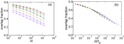
Figure 3: Aging plot: (a) Average overlap fraction $C(t_{\rm w},\Delta t)/L(t_{\rm w})$ for different $t_{\rm w}$’s (from $1\times$ to $512\times$ $25,600$ Monte-Carlo steps) deep in the glass phase, with ${\cal T}=0.9{\cal T}_{\rm d}>{\cal T}_{\rm loc}$; (b) Scaling plot of (a) with $\Delta t$ normalized by $t_{\rm w}$.

In Fig. 3(a), we show the overlap fraction, parameterized by the different waiting time $t_{\rm w}$’s for the system biased deep in the glass phase with ${\cal T}=0.9\ {\cal T}_{\rm d}$. The overlap fraction clearly depends on the waiting time, illustrating the glassy nature of the dynamics. In contrast, the same quantity computed for ${\cal T}<{\cal T}_{\rm d}$ (data not shown) gives no statistically significant dependence on $t_{\rm w}$. To characterize more quantitatively the behavior, we re-plot in Fig. 3(b) the curves in (a) with $\Delta t$ normalized by $t_{\rm w}$. We find these curves to collapse reasonably onto a single master curve which exhibits a weak kink at $\Delta t/t_{\rm w}\sim 1$. A naive explanation of this behavior is that for $\Delta t\ll t_{\rm w}$, the bubble stays approximately within the energy valley found at time $t_{\rm w}$, while for $\Delta t\gg t_{\rm w}$, the bubble makes excursion far away from the valley. For the one-dimensional “trap” model, it was shown rigorously corr-scale that $C(t_{\rm w},\Delta t)$ indeed scales as a function of $\Delta t/t_{\rm w}$, even though the largest trap time actually scales sub-linearly with $t_{\rm w}$. This behavior can be understood in terms of the particle making multiple returns to the original valley after escaping it berbou , as manifested by the slow decay shown in Fig. 3(b) for $\Delta t\gg t_{\rm w}$.

IV Discussion

In this study we investigated the thermodynamic and dynamic behaviors of twist-induced denaturation bubbles in a long, random sequence of DNA. The small bubbles associated with weak twist are delocalized, e.g., they flicker in and out of existence according to the Boltzmann distribution and are independent of the DNA sequence. The bubbles increase in lengths upon increase in the applied torque. When the largest bubbles reach a critical size $L_{\rm loc}$ which is of the order of a few tens of bases, the bubbles become localized to AT-rich segments which occur statistically in a long random sequence. According to the parameters SantaLucia taken at $37^{\circ}{\tt C}$ with $[{\rm Na}^{+}]=1~{}{\tt M}$, the localization “transition” occurs at ${\cal T}_{\rm loc}\approx 8\ {\rm pN}\cdot{\rm nm}$, which is $\sim 80\%$ of the torque needed for bulk denaturation ${\cal T}_{\rm d}$. In the localized regime, the bubbles exhibit “aging” and move along the double helix sub-diffusively, with continuously varying dynamic exponents.

All of the results are obtained under the single-bubble approximation. Thermodynamically, we expect this approximation to be valid for DNA sequences of several thousand bases or less. This is due to the strongly cooperative nature of bubble formation, as manifested in the large initiation energy $\gamma_{1}$. The single bubble description of dynamics is further restricted by the finite life time of the bubble: Even at length scales where the single-bubble approximation is appropriate thermodynamically, the bubble may annihilate and reappear elsewhere in the sequence, effectively performing long-distance hops. Experimental knowledge of the bubble life time in the presence of an applied twist is needed to estimate the crossover time to the long-distance hopping regime. Qualitatively, we expect these bubbles to have much longer life times than the thermally denatured bubbles, since the applied twist plays the role of an energy barrier preventing bubble annihilation.

Finally, we note that bubble localization characterized in this study is a reflection of the statistical background present in long random nucleotide sequences. This background traps the bubble kinetically if the bubble size becomes sufficiently large. Thus, to localize denaturation bubbles at appropriate locations specified by designed sequences (e.g., promoters or replication origins) for biological functions, it is necessary to operate away from the localized regime, i.e., below the onset of localization.

This collaboration was made possible by the program on “Statistical Physics and Biological Information” hosted by the Institute for Theoretical Physics in Santa Barbara. The authors benefitted from discussions with D. Bensimon, R. Bundschuh, H. Chate, U. Gerland, D. Lubensky, M. Mezard, and Y.-k. Yu. TH is supported by NSF Grant No. 0211308 and a Burroughs-Wellcome functional genomics award. LT acknowledges the hospitality of UC San Diego where part of this work was carried out.

References

- [1] Alberts, B. et al (2002) Molecular Biology of the Cell, (Garland Science).
- [2] Kowalski, D., Natale, D.A., and Eddy, M.J. (1988) Proc. Natl. Acad. Sci. (USA) 85, 9464–9468.
- [3] Kanaar R. and Cozzarelli N.R. (1992) Curr. Op. Struct. Biol. 2, 369–379.
- [4] Strick T., Allemand J.F., Bensimon D., Bensimon A. and Croquette V. (1996) Science 271, 1835–1837.
- [5] Marko, J.F. and Siggia, E.D. (1995) Phys. Rev. E 52, 2912–2938.
- [6] Cocco S. and Monasson, R. (1999) Phys. Rev. Lett. 83 5178–5181.
- [7] Strick, T.R., Allemand, J.F., Bensimon, D. and Croquette, V. (2000) Annu. Rev. Biophys. Biomol. Strut. 29, 523–543.
- [8] Fye, R.M. and Benham, C.J. (1999) Phys. Rev. E 59, 3408–3426.
- [9] Cule, D. and Hwa, T. (1997) Phys. Rev. Lett. 79, 2375–2378.
- [10] Tang, L.-H. and Chaté, H. (2001) Phys. Rev. Lett. 86, 830–833.
- [11] Bockelmann U., Thomen P., Essevaz-Roulet B., Viasnoff V. and Heslot F. (2002) Biophys. J 82, 1537–1553.
- [12] Lubensky, D.K. and Nelson, D.R. (2002) Phys. Rev. E 65, 031917.
- [13] Binder, K. and Young, A.P. (1986) Rev. Mod. Phys. 58, 801–976.
- [14] Struick, L.C.E. (1978) Physical Ageing in Amorphous Polymers and Other Materials, (Elsevier, Houston).
- [15] Bouchaud, J.-P., Cugliandolo, L.F., Kurchan, J. and Mézard, M. (1998) in Spin Glasses and Random Fields, ed. Young, A.P. (World Scientific, Singapore), pp. 2613–2626.
- [16] Derrida, B. (1981) Phys. Rev. B 24, 2613–2626.
- [17] Karlin, S. and Altschul, S.F. (1990) Proc. Natl. Acad. Sci. (USA) 87, 2264–2268.
- [18] Yu, Y.-k. and Hwa, T. (2001) J. Comp. Biol. 8, 249–282.
- [19] SantaLucia, J., Jr., Hatim, T.A. and Senevirante, P.A. (1996) Biochem. 35, 3555–3562.
- [20] SantaLucia, J., Jr. (1998) Proc. Natl. Acad. Sci. (USA) 95, 1460–1465.
- [21] Blake, R.D., Bizzaro, J.W., Blake, J.D., Day, G.R., Delcourt, S.G., Knowles, J., Marx, K.A., SantaLucia, J., Jr. (1999) Bioinformatics 15, 370–375.
- [22] Fisher, M.E. (1966) J. Chem. Phys. 45, 1469–1473.
- [23] Kafri, Y., Mukamel, D. and Peliti L. (2000) Phys. Rev. Lett. 85, 4988–4991.
- [24] Garel, T., Monthus, C. and Orland, H. (2001) Europhys. Lett. 55, 132–138.
- [25] Rouzina, I. and Bloomfield, V.A. (2001) Biophys. J. 80, 882–893.
- [26] Gerland, U., Moroz, J.D. and Hwa, T. (2002) Proc. Natl. Acad. Sci. (USA) 99, 12015–12020.
- [27] Karlin, S. and Dembo, A. (1992) Adv. Appl. Probab. 24, 113–140.
- [28] Karlin, S. and Altschul, S.F. (1993) Proc. Natl. Acad. Sci. (USA) 90, 5873–5677.
- [29] Marinari, E. and Parisi, G. (1993) J. Phys. A 26, L1149–L1156.
- [30] Alexander, S. (1981) Phys. Rev. B 23, 2951–2960.
- [31] Machta, J. (1985) J. Phys. A 18, L531-534.
- [32] Bertin, E.M. and Bouchaud, J.-P. (2002) at http://lanl.arXiv.org/pdf/cond-mat/0210521
- [33] Fontes, L.R.G., Isopi, M. and Newman, C.M. (2002) Ann. Probab. 30, 579–604.