A three-dimensional wavelet based multifractal method : about the need of revisiting the multifractal description of turbulence dissipation data

Abstract

We generalize the wavelet transform modulus maxima (WTMM) method to multifractal analysis of 3D random fields. This method is calibrated on synthetic 3D monofractal fractional Brownian fields and on 3D multifractal singular cascade measures as well as their random function counterpart obtained by fractional integration. Then we apply the 3D WTMM method to the dissipation field issued from 3D isotropic turbulence simulations. We comment on the need to revisiting previous box-counting analysis which have failed to estimate correctly the corresponding multifractal spectra because of their intrinsic inability to master non-conservative singular cascade measures.

The multifractal formalism was introduced in the mid-eighties to provide a statistical description of the fluctuations of regularity of singular measures found in chaotic dynamical systems ref1 or in modelling the energy cascading process in turbulent flows ref2 ; aMen91 ; bFri95 . Box-counting (BC) algorithms were successfully adapted to resolve multifractal scaling for isotropic self-similar fractals aMen91 ; ref5 . As to self-affine fractals, Parisi and Frisch aPar85 developed, in the context of turbulence velocity data analysis, an alternative multifractal description based on the so-called structure functions. Unfortunately, there are some drawbacks to these classical multifractal methods and as proposed in Ref. ref9 , a natural way of performing a unified multifractal analysis of both singular measures and multi-affine functions, consists in using the continuous wavelet transform (WT). Applications of the so-called WTMM method to 1D signals have already provided insight into a wide variety of problems, e.g. fully-developed turbulence, financial markets, meteorology, physiology, DNA sequences bArn95 . Recently, the WTMM method has been generalized to 2D for multifractal analysis of rough surfaces ref14 , and successfully applied to characterize the intermittent nature of satellite images of the cloud structure ref15 and to assist in the diagnosis in digitized mammograms akes01 . Our aim here is to go one step further and to generalize the WTMM method from 2D to 3D.

The 3D WTMM method consists in smoothing the discrete 3D field data by convolving it with a filter and then in computing the gradient on the smoothed signal as for multiscale edge detectors ref10 . Define three wavelets $\psi_{i}(x,y,z)=\partial\phi(x,y,z)/\partial x_{i}$ with $x_{i}=x,y$ or $z$ for $i=1,2$ or 3 respectively and $\phi(x,y,z)$ is a 3D smoothing function well localized around $x=y=z=0$. For any function $f(x,y,z)\in L^{2}$($\mathbb{R}$³), the WT at the point ${\mathbf{b}}$ and scale $a$ can be expressed in a vectorial form ref14 ; ref10 :

$${\mathbf{T}}_{\boldsymbol{\psi}}[f]({\mathbf{b}},a)={\boldsymbol{\nabla}}\{\phi_{{\mathbf{b}},a}*f\}\;,$$ (1)

where $\phi_{{\mathbf{b}},a}({\mathbf{r}})=a^{-3}\phi(a^{-1}({\mathbf{r}}-{\mathbf{b}}))$. If $\phi$ is just a Gaussian $\phi({\mathbf{r}})=\exp(-{\mathbf{r}}^{2}/2)$ (or one of its derivatives), then Eq. (1) defines the 3D WT as the gradient field vector of $f({\mathbf{r}})$ smoothed by dilated versions $\phi({\mathbf{r}}/a)$ of this filter. At a given scale $a$, the WTMM are defined by the positions ${\mathbf{b}}$ where the WT modulus ${\mathcal{M}}_{\boldsymbol{\psi}}[f]({\mathbf{b}},a)=|{\mathbf{T}}_{\boldsymbol{\psi}}[f]({\mathbf{b}},a)|$ is locally maximum along the direction of the WT vector (Eq. (1)). These WTMM lie on connected surfaces called maxima surfaces (see Fig. 2). In theory, at each scale $a$, one only needs to record the position of the local maxima of ${\mathcal{M}}_{\boldsymbol{\psi}}$ (WTMMM) along the maxima surfaces together with the value of ${\mathcal{M}}_{\boldsymbol{\psi}}[f]$ and the WT vector direction. They indicate locally the direction where the signal has the sharpest variation. These WTMMM are disposed along connected curves across scales called maxima lines ref10 ; ref14 living in a 4D space $(x,y,z,a)$. We will define the WT skeleton as the set of maxima lines that converge to the $(x,y,z)$-hyperplane in the limit $a\rightarrow 0^{+}$ (Fig 2(d)). One can prove ref10 ; ref14 that, provided the first $n_{\boldsymbol{\psi}}$ moments of $\boldsymbol{\psi}$ be zero, then ${\mathcal{M}}_{\boldsymbol{\psi}}[f]\bigl{(}{\mathcal{L}}_{{\mathbf{r}_{0}}}(a)\bigr{)}\sim a^{h({\mathbf{r}_{0}})}$ along the maxima line ${\mathcal{L}}_{{\mathbf{r}_{0}}}(a)$ pointing to the point ${\mathbf{r}}_{0}$ in the limit $a\rightarrow 0^{+}$, where $h({\mathbf{r}}_{0})$ ($<n_{\boldsymbol{\psi}}$) is the local Hölder exponent of $f$. As in 1D and 2D ref9 ; ref14 , the 3D WTMM method consists in defining the partition functions :

$${\mathcal{Z}}(q,a)=\sum_{{\mathcal{L}}\in{\mathcal{L}}(a)}\left({\mathcal{M}}_{\boldsymbol{\psi}}[f]({\mathbf{r}},a)\right)^{q}\sim a^{\tau(q)},$$ (2)

where $q\in$ $\mathbb{R}$  and ${\mathcal{L}}(a)$ is the set of maxima lines of the WT skeleton. Then from Legendre transforming $\tau(q)$: $D(h)=\min_{q}\bigl{(}qh-\tau(q)\bigr{)}$, one gets the $D(h)$ singularity spectrum defined as the Hausdorff dimension of the set of points ${\mathbf{r}}$ where $h({\mathbf{r}})$ is $h$. As an alternative strategy one can compute the mean quantities $h(q,a)$ and $D(q,a)$ :

$$h(q,a)= \sum_{{\mathcal{L}}\in{\mathcal{L}}(a)}\ln\left|{\mathcal{M}}_{\boldsymbol{\psi}}[f]({\mathbf{r}},a)\right|\;W_{\boldsymbol{\psi}}[f](q,{\mathcal{L}},a)\;,$$ (3)

$$D(q,a)= \sum_{{\mathcal{L}}\in{\mathcal{L}}(a)}W_{\boldsymbol{\psi}}[f](q,{\mathcal{L}},a)\;\ln\bigl{(}W_{\boldsymbol{\psi}}[f](q,{\mathcal{L}},a)\bigr{)}\;,$$ (4)

where $W_{\boldsymbol{\psi}}[f](q,{\mathcal{L}},a)=\bigl{(}{\mathcal{M}}_{\boldsymbol{\psi}}[f]({\mathbf{r}},a)\bigr{)}^{q}/{\mathcal{Z}}(q,a)$ is a Boltzmann weight computed from the WT skeleton. From the scaling behavior of these quantities, one can extract $h(q)=\lim_{a\rightarrow 0^{+}}h(q,a)/\ln a$ and $D(q)=\lim_{a\rightarrow 0^{+}}D(q,a)/\ln a$ and therefore the $D(h)$ spectrum.

Fractional Brownian motions (fBm) are homogenous random self-affine functions that have been used to calibrate both the 1D and 2D WTMM methods ref9 ; ref14 . 3D fBm $B_{H}({\mathbf{r}})$ are Gaussian stochastic processes with stationary increments and well-known statistical properties : $\tau(q)=qH-3\;,\;0<H<1$. In Fig. 1 are reported the results of the 3D WTMM method when applied to 16 $\times$ $(256)^{3}$ realizations of $B_{H=1/2}({\mathbf{r}})$. As shown in Fig. 1(a), ${\mathcal{Z}}(q,a)$ (Eq. (2)) display nice scaling behavior over 3 octaves when plotted vs $a$ in a logarithmic representation. A linear regression fit of the data yields the linear $\tau(q)$ spectrum shown in Fig. 2(c), in good agreement with the theoretical spectrum. This signature of monofractality is confirmed in Fig. 1(b) where, when plotting $h(q,a)$ vs $\log_{2}(a)$, $H=1/2$ is shown to provide an excellent fit of the slope of the data ($\sigma_{W}\lesssim a\lesssim 4\sigma_{W}$) for $q\in]-2,4[$. When using $h(q,a)$ (Eq. (3)) and $D(q,a)$ (Eq. (4)) to estimate $h(q)$ and $D(q)$ in Fig. 1(d), one gets, up to the numerical uncertainty, a $D(h)$ spectrum that reduces to a single point $D(h=H=1/2)=3$. Similar quantitative estimates have been obtained for $H=1/3$ and $2/3$, thus confirming that 3D fBm’s are nowhere differentiable with a unique Hölder exponent $h=H$.

Generating multifractal measures using multiplicative cascades is well documented ref2 ; aMen91 ; bFri95 . The “binomial (or p-) model”, originally designed to account for the statistical scaling properties of the dissipation field in fully developed turbulence, has very simple multifractal properties ref2 ; aMen91 ; bFri95 .

Figure 1: Multifractal analysis of 3D $B_{H=1/2}$ (

$\blacksquare$

), 3D p-model ($\bullet$, $p=0.32$) and 3D FISC ($\circ$, $p=0.32$, $H^{*}=0.638$) data using the 3D WTMM method with a first (

$\blacksquare$

) or third ($\bullet$,$\circ$) order analyzing wavelet ($\phi({\mathbf{r}})$ is a Gaussian or its Laplacian). (a) $\log_{2}{\cal Z}(q,a)$ vs $\log_{2}a$; (b) $h(q,a)$ vs $\log_{2}a$; the dashed and solid lines correspond to linear regression fits over the three first octaves. (c) $\tau(q)$ vs $q$; the dashed and solid lines are the theoretical predictions. (d) $D(h)$ vs $h$ as obtained from the scaling behavior of $h(q,a)$ and $D(q,a)$. These results correspond to annealed averaging over $16$ $\times$ $(256)^{3}$ images. $a$ is expressed in $\sigma_{W}$ units where $\sigma_{W}=7$ (pixels) is the characteristic size of $\boldsymbol{\psi}$ at the smallest resolved scale. In (c) and (d), the symbols (

$\blacktriangle$

) represent the results of classical box-counting analysis of the 3D p-model.

The 3D version of the p-model consists in starting with a cube of size $L$, in which a measure $\mu=\mu_{L}$ is uniformly distributed. At the first step, the initial cube is broken into eight smaller cubes of size $L/2$ and one selects at random the four sub-cubes which will receive a fraction $M^{(1)}=p_{1}/4$, the four others receiving the fraction $M^{(2)}=p_{2}/4$ of the measure ($p_{1}+p_{2}=1$). Iterating this rule, one generates a random singular measure $\mu_{n}({\mathbf{r}};l)=\mu_{L}\prod_{i=1}^{n}M_{i}\;,\;l/L=2^{-n}\rightarrow 0$. A straightforward computation yields : $\tau_{\mu}(q)=-(q+2)-\log_{2}\bigl{(}p_{1}^{q}+p_{2}^{q}\bigr{)}$. As a mean of introducing continuity, Fractionaly Integrated Singular Cascade (FISC) algorithm aSch87 amounts to a low-pass power-law filtering in Fourier space: $f_{n}({\mathbf{r}})=\mu_{n}({\mathbf{r}})*|{\mathbf{r}}|^{-(1-H^{*})}\;,\;0<H^{*}<1$. This leads to FISC random functions with the following multifractal spectrum : $\tau_{f}(q)=\tau_{\mu}(q)+qH^{*}=-2-q(1-H^{*})-\log_{2}\bigl{(}p_{1}^{q}+p_{2}^{q}\bigr{)}$. In Fig. 1 are reported the results of the 3D WTMM analysis of the FISC model with $p_{1}=0.32$ and $H^{*}=0.638$. As shown in Fig. 1(a), ${\mathcal{Z}}(q,a)$ display good scaling for $q\in]-2,4[$ for which statistical convergence turns out to be achieved. The corresponding $\tau_{f}(q)$ spectrum is displayed in Fig. 1(c) along with the theoretical spectrum. The agreement is quite satisfactory; $\tau_{f}(q)$ is nonlinear, the hallmark of multifractal scaling. This is confirmed in Fig. 1(b) where the slope of $h(q,a)$ vs $\log_{2}(a)$ clearly depends on $q$. From the estimate of $h(q)$ and $D(q)$, one gets the single-humped $D_{f}(h)$ spectrum shown in Fig. 1(d). Note that some departure from the theoretical spectrum can be observed on the right-hand side of the $D(h)$-curve ($q\lesssim-2$) indicating that the estimate of the weakest singularities would require a larger statistical sample. In Figs. 1(c) and 1(d) are also reported the results of a comparative analysis of the p-model using the 3D WTMM method and classical BC techniques. Note that the WTMM definition of the $\tau_{\mu}^{WT}(q)$ spectrum (Eq. (2)) slightly differs from the BC definition $\tau_{\mu}^{BC}(q)$ found in the literature aMen91 :

$$\tau_{\mu}^{BC}(q)=\tau_{\mu}^{WT}(q)+dq=(q-1)D_{q}\;,$$ (5)

which implies the following relationship $f_{\mu}^{BC}(\alpha)=D_{\mu}^{WT}(h=\alpha-d)$ between the corresponding singularity spectra ($d=3$). For both methods, the numerical results for $\tau_{\mu}(q)$ and $D_{\mu}(h)$ are found in good agreement with the theoretical spectra, for $q\in]-2,4[$. In particular, the cancellation exponent ref26 is found $\tau_{\mu}^{BC}(q=1)=\tau_{\mu}^{WT}(q=1)+3=0$, as the signature of the conservativity of the p-model cascading rule. One of the main problem with the BC method is the fact that, by construction, the measure in a given box is the sum of the measures in smaller non-overlapping boxes, which implies that the cancellation exponent $\tau_{\mu}^{BC}(q=1)=0$. This means that BC algorithms are not adapted to study non-conservative singular cascades, signed measures as well as multifractal functions for which the cancellation exponent has no reason to vanish. Altogether the results reported in Fig. 1 bring the demonstration that our 3D WTMM methodology paves the way from multifractal analysis of singular measures to continuous multi-affine functions. In particular the $D_{f}(h)$ curve for the FISC random function is found identical to the $D_{\mu}(h)$ curve up to a translation to the right by $H^{*}$; this is the consequence of the fractional integration which implies $D_{f}(h)=D_{\mu}(h-H^{*})$.

Since Kolmogorov’s founding work (K41), fully developed turbulence has been intensively studied theoretically, numerically and experimentally aMen91 ; bFri95 . A central quantity in the K41 theory is the mean energy dissipation $\epsilon=\frac{\nu}{2}\sum_{i,j}(\partial_{j}v_{i}+\partial_{i}v_{j})^{2}$ which is supposed to be constant. Indeed, $\epsilon$ is not spatially homogenous but undergoes local intermittent fluctuations aMen91 ; bFri95 . There have been early experimental attemps to measure the multifractal spectra of $\epsilon$ aMen91 . Surprisingly, the binomial model turns out to account reasonably well for the observed $\tau_{\epsilon}(q)$ and $f_{\epsilon}(\alpha)$ spectra aMen91 . Experimentally, single probe measurement of the longitudinal velocity requires the use of the 1D surrogate dissipation approximation $\epsilon^{\prime}=15\nu(\partial u/\partial x)^{2}$ that may introduce severe bias in the multifractal analysis. 3D multifractal processing of dissipation data is at the moment feasible only for numerically simulated flows at moderate Reynolds number for which scaling just begins to manifest itself ref20 . Several numerical studies [16a,c] agree that $\epsilon^{\prime}$ is in general more intermittent than $\epsilon$ which is found nearly log-normal in the inertial range [16b,c].

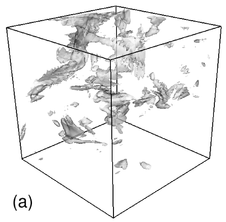
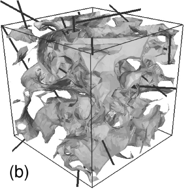
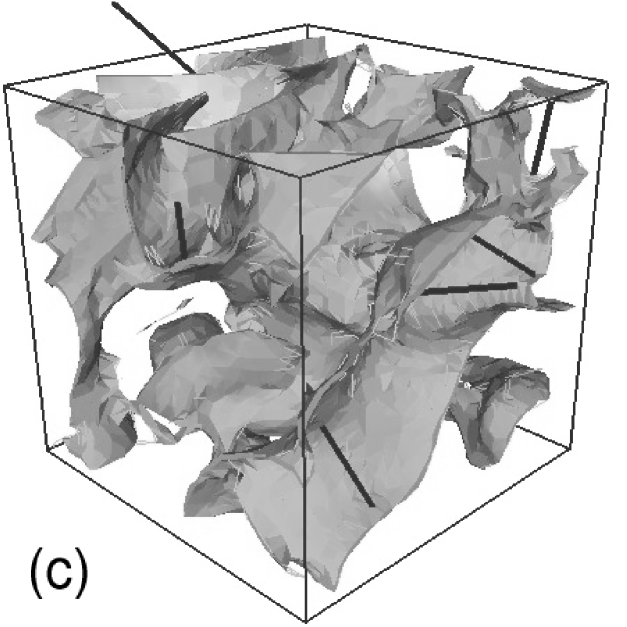
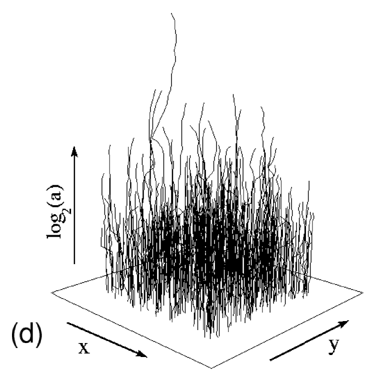
Figure 2: 3D WT analysis of the DNS dissipation field $\epsilon$. $\boldsymbol{\psi}$ is the first-order analyzing wavelet ($\phi({\mathbf{r}})$ is the Gaussian). (a) Isosurface plot of $\epsilon$ in a $(64)^{3}$ sub-cube. (b) WTMM surfaces at scale $a=2\sigma_{W}$; from the local maxima (WTMMM) of ${\mathcal{M}}_{\boldsymbol{\psi}}$ along these surfaces originate a black segment whose length is proportional to ${\mathcal{M}}_{\boldsymbol{\psi}}$ and direction is along the WT vector. (c) same as in (b) for $a=4\sigma_{W}$. (d) 3D projection of the WT skeleton obtained by linking the WTMMM across scales.

So far mainly BC techniques have been used to perform multifractal analysis of numerical and experimental dissipation data aMen91 ; ref20 . Here we apply the 3D WTMM method to isotropic turbulence DNS data obtained by Meneguzzi with the same numerical code as in Ref. aMene but at a $(512)^{3}$ resolution and a viscosity of $5.10^{-4}$ corresponding to a Taylor Reynolds number $R_{\lambda}=216$ (one snapshot of the dissipation 3D spatial field). For the sake of comparison, we will also report the results of some averaging over 18 snapshots of ($256$)³ DNS run by Lévêque at $R_{\lambda}=140$. The main steps of our 3D WT computation are illustrated in Fig. 2. Focusing on a ($64^{3}$) sub-cube, we show the original $\epsilon$ data (Fig. 2(a)), the WTMM surfaces along with the WTMMM points computed at two different scales (Figs. 2(b) and 2(c)) and some projection of the WT skeleton (Fig. 2(d)). According to Eq. (5), by plotting ${\mathcal{Z}}(q,a)/({\mathcal{Z}}(q=0,a))^{q}$ vs $a$ in a logarithmic representation in Fig. 3(a), one can then directly compare (${\mathcal{Z}}(q=0,a)\sim a^{-d}$) our WTMM computations with BC ones. Actually, good scaling properties are observed for $q\in]-2,4[$. Linear regression fits of the data yield the non-linear $\tau_{\epsilon}(q)$ spectra shown in Fig. 3(c) that significantly deviate from a straight line, the hallmark of multifractality. But surprisingly, $\tau_{\epsilon}^{WT}(q)$ significantly differs from $\tau_{\epsilon}^{BC}(q)-3q$. Actually, our 3D WTMM algorithms reveal that the cancellation exponent ref26 is significantly different from zero : $\tau_{\epsilon}^{WT}(q=1)+3=-0.19\pm 0.03<0$, the signature of a signed measure.

Figure 3: Multifractal analysis of Meneguzzi DNS dissipation data ($d=3$) using the 3D WTMM method ($\triangle$) and BC techniques ($\blacktriangle$). (a) $\log_{2}({\cal Z}(q,a)/({\cal Z}(q=0,a))^{q})$ vs $\log_{2}a$; (b) $h(q,a)=\alpha(q,a)-3$ vs $\log_{2}a$; the solid and dashed lines correspond to linear regression fits over $\sigma_{W}\lesssim a\lesssim 2^{3}\sigma_{W}$. (c) $\tau_{\epsilon}(q)=\tau_{\epsilon}^{WT}(q)$ or $\tau_{\epsilon}^{BC}(q)-3q$ vs $q$; the solid (dashed) lines correspond to the p-model prediction with $p_{1}=0.36$, $p_{2}=0.78$ ($p_{1}=0.32$, $p_{2}=0.68$). (d) $f_{\epsilon}(\alpha)+3-d$ vs $\alpha-d+1$, where $f_{\epsilon}(\alpha)=f_{\epsilon}^{BC}(\alpha)$ or $f_{\epsilon}^{WT}(\alpha)=D_{\epsilon}^{WT}(h=\alpha-d)$ ; the solid and dashed lines have the same meaning as in (c); the thick solid line is the log-normal spectrum $f_{\epsilon}(\alpha)=d-(\alpha-d+1-C_{1})^{2}/2C_{2}$ with $C_{1}=0.91$ and $C_{2}=0.22$. The symbols (

$\square$

) correspond to some average $f(\alpha)$ spectrum of experimental ($d=1$) surrogate dissipation data aMen91 . In (c) and (d), the 3D WTMM multifractal spectra of Lévêque 3D dissipation data (18 snapshots) ($\circ$) are shown for comparison. In (d) the dashed straight line is the diagonal.

Indeed, as shown in Fig. 3(c), $\tau_{\epsilon}^{WT}(q)$ data are rather nicely fitted by the theoretical spectrum $\tau_{\mu}(q)$ of the non-conservative p-model with $p_{1}=0.36$ and $p_{2}=0.78$ ($p_{1}+p_{2}=1.14>1$). Thus BC algorithms systematically provide a misleading conservative $\tau_{\epsilon}(q)$ spectrum diagnostic with $p=p_{1}/(p_{1}+p_{2})$ and $1-p=p_{2}/(p_{1}+p_{2})$. As shown in Fig. 3(c), $\tau_{\epsilon}^{BC}(q)-3q$ data are quite well reproduced by the theoretical conservative p-model spectrum with $p=0.32=p_{1}/(p_{1}+p_{2})=0.36/1.14$, consistently with our 3D WTMM finding for $\tau_{\epsilon}^{WT}(q)$. The difference between the two spectra is nothing but a fractional integration of exponent $H^{*}=\log_{2}(p_{1}+p_{2})\sim 0.19$. This result is confirmed in Fig. 3(d) where the singularity spectrum $f_{\epsilon}^{BC}(\alpha)$ is misleading shifted to the right by $H^{*}$ ($=-$ the cancellation exponent) $\sim 0.19$, without any shape change as compared to the $f_{\epsilon}^{WT}(\alpha)=D_{\epsilon}^{WT}(h=\alpha-d)$. Note that the observation that $f_{\epsilon}^{WT}(\alpha-d+1)$ is not tangent to the diagonal (on the contrary to $f_{\epsilon}^{BC}(\alpha-d+1)$) is clearly related to the fact that the cancellation exponent is different from zero aZhou01 . This observation seriously questions the validity of most of the experimental and numerical BC estimates of the $\tau_{\epsilon}^{BC}(q)$ and $f_{\epsilon}^{BC}(\alpha)$ spectra reported so far in the literature. In Fig. 3(d) is shown for comparison some average $f_{\epsilon}^{BC}(\alpha)$ spectrum obtained by Meneveau and Sreenivasan aMen91 for 1D surrogate dissipation experimental data ($d=1$). We notice that these experimental data were claimed to be well fitted by the conservative p-model with $p=0.3$ ($1-p=0.7$), i.e. a value not so far from the value $p=p_{1}/(p_{1}+p_{2})=0.32$ derived from our 3D WTMM method.

Previous application of the 1D WTMM method to 1D surrogate dissipation data has already revealed the fact that the cancellation exponent might be different from zero tRou96 . The 3D WTMM results reported here show that this surprising result is not some artefact resulting from the analysis of 1D cuts (the dissipation could well be non conserved along these cuts), but that the multifractal spatial structure of the 3D dissipation field is likely to be well described by a multiplicative cascade process that is definitely non conservative. As shown in Fig. 3(d), this conclusion is confirmed by the results obtained when averaging over 18 snapshots of Lévêque’s DNS; the cancellation exponent is found even more negative $\tau_{\epsilon}^{WT}(q=1)+3=-0.26$, as an indication (as regards to the smaller $R_{\lambda}$ value) that this exponent might decrease to zero in the limit of infinite Reynolds number. To conclude, let us point out that the $f_{\epsilon}^{WT}(\alpha)$ data seem to be even better fitted by a parabola, as predicted for non-conservative log-normal cascade processes.

We are very grateful to M. Meneguzzi and E. Lévêque for allowing us to have access to their DNS data and to the CNRS under GDR turbulence.

References

- (1) T. C. Halsey et al., Phys. Rev. A 33, 1141 (1986).
- (2) B. B. Mandelbrot, J. Fluid Mech. 62, 331 (1974).
- (3) C. Meneveau and K. R. Sreenivasan, J. Fluid Mech. 224, 429 (1991).
- (4) U. Frisch, Turbulence (Cambridge Univ. Press, Cambridge, 1995).
- (5) P. Grassberger and I. Procaccia, Physica (Amsterdam) 9D, 189 (1983).
- (6) G. Parisi and U. Frisch, in Turbulence and Predictability in Geophysical Fluid Dynamics and Climate Dynamics, edited by M. Ghil et al (North-Holland, Amsterdam, 1985), p. 84.
- (7) J. F. Muzy, E. Bacry, and A. Arneodo, Int. J. Bifurcation Chaos Appl. Sci. Eng. 4, 245 (1994); A. Arneodo, E. Bacry, and J. F. Muzy, Physica (Amsterdam) 213A, 232 (1995).
- (8) (a) A. Arneodo et al., Ondelettes, Multifractales et Turbulences : de l’ADN aux croissances cristallines (Diderot Editeur, Art et Sciences, Paris, 1995); (b) The Science of Disasters : climate disruptions, heart attacks and market crashes, edited by A. Bunde et al (Springer Verlag, Berlin, 2002).
- (9) A. Arneodo, N. Decoster, and S. G. Roux, Eur. Phys. J. B 15, 567 (2000); N. Decoster, S. G. Roux, and A. Arneodo, Eur. Phys. J. B 15, 739 (2000).
- (10) A. Arneodo, N. Decoster, and S. G. Roux, Phys. Rev. Lett. 83, 1255 (1999); S. G. Roux, A. Arneodo, and N. Decoster, Eur. Phys. J. B 15, 765 (2000).
- (11) P. Kestener et al., Image Anal. Stereol. 20, 169 (2001).
- (12) S. Mallat and W. L. Hwang, IEEE Trans. on Information Theory 38, 617 (1992).
- (13) D. Schertzer, and S. Lovejoy, J. Geophys. Res. 92, 9693 (1987).
- (14) E. Ott et al., Phys. Rev. Lett. 69, 2654 (1992).
- (15) (a) S. Chen et al., Phys. Fluids A 5, 458 (1992); (b) L. P. Wang et al., J. Fluid Mech. 309, 113 (1996); (c) I. Hosokawa, S. et al., Phys. Rev. Lett. 77, 4548 (1996);
- (16) A. Vincent and M. Meneguzzi, J. Fluid Mech. 225, 1 (1995).
- (17) W. X. Zhou and Z. H. Yu, Physica (Amsterdam) 294A, 273 (2001).
- (18) S. G. Roux, Ph.D. thesis, University of Aix-Marseille II, 1996, unpublished.