A simulation study of localization of electromagnetic waves in two-dimensional random dipolar systems

Abstract

We study the propagation and scattering of electromagnetic waves by random arrays of dipolar cylinders in a uniform medium. A set of self-consistent equations, incorporating all orders of multiple scattering of the electromagnetic waves, is derived from first principles and then solved numerically for electromagnetic fields. For certain ranges of frequencies, spatially localized electromagnetic waves appear in such a simple but realistic disordered system. Dependence of localization on the frequency, radiation damping, and filling factor is shown. The spatial behavior of the total, coherent and diffusive waves is explored in detailed, and found to be comply with a physical intuitive picture. A phase diagram characterizing localization is presented, in agreement with previous investigations on other systems.

I Introduction

The concept of localization was originally introduced by AndersonAnderson for electrons in a crystal. In the case of a perfectly periodic lattice, except in the gaps all the electronic states are extended and are represented by Bloch states. When a sufficient amount of disorders is added to the lattice, for example in the form of random potentials, the electrons may become spatially localized due to the multiple scattering by the disorders. In such a case, the eigenstates are exponentially confined in the spaceLee . The inception of the localization concept has opened a new era for the study of electrons in disordered systems, and stimulated a tremendous research. The concept of localization has also rendered a great development in many other fields such as seismologySeis , oceanologyocean , and random lasersLaser , to name just a few. The great efforts have been summarized in a number of excellent reviews (e. g. Lee ; Thouless ; John ; Sheng ; Lagen ; Rossum ; Van ; loc ).

Over the past two decades, localization of classical waves has been under intensive investigations, leading to a very large body of literature(e. g. John ; Sheng ; Lagen ; HW ; Kirk1 ; He ; Condat ; Sor ; Genack ; McCall ; McCall2 ; Marian ; Sigalas ; AAA ; Ye1 ; Wiersma ; weak ; AAC ). Such a localization phenomenon has been characterized by two levels. One is the weak localization associated with the enhanced backscattering. That is, waves which propagate in the two opposite directions along a loop will obtain the same phase and interfere constructively at the emission site, thus enhancing the backscattering. The second is the strong localization, without confusion often just termed as localization, in which a significant inhibition of transmission appears and the energy is mostly confined spatially in the vicinity of the emission site.

While the weak localization, regarded as a precursor to the strong localization, has been well studied both theoretically (e. g. the monographSheng ) and experimentally (e. g. weak ), observation of strong localization of classical waves for higher than one dimension remains a subject of debateWiersma ; AAC ; debate , primarily because a suitable system is hard to find and the observation is often obscured by such effects as the residual absorptiondebate and scattering attenuation. Asides from few exceptionsMcCall , most experiments are based on observations of the exponential decay of waves as they propagate through disordered media. This was pointed out in Ref. AAC . According to Chen2002 , this type of experiments is not sufficient to discern whether the medium really only has localized states. Unwanted effects of non-localization origin can also contribute to the exponential decay, making data interpretation possibly ambiguous. In a conclusion, Sigalas et al. Sigalas pointed out that there is no conclusive experimental evidence for localization of electromagnetic waves (EM) in two dimensions (2D). We mention that there was a report of the observation of microwave localization in two dimensions when a transmitting source is inside disordered mediaMcCall .

The difficulties in observing localization of EM waves mainly lie in a couple of problems. First, wave localization only appears for strongly scattering media, and such a medium is often hard to find. Second, localization effects are often entangled with other effects such as dissipation, wave deflection, or boundary effectsloc , making data interpretation often ambiguous. In a recent communication, a simple but seemingly realistic model system has been proposed to study EM localization in 2D random mediaYLS . This model originated from the previous study of the radiative effects of the electric dipoles embedded in structured cavitiesErdogan . It was shown that EM localization is possible in such a disordered system. When localization occurs, a coherent behavior appears and is revealed as a unique property differentiating localization from either the residual absorption or the attenuation effects.

With the present paper, we wish to explore further the localization properties of the system outlined in YLS . We will investigate the dependence of localization behavior on a numbers of parameters including frequency, filling factor, scattering strength, damping effect, and two different ways of measuring localization. Additionally, the spatial behaviors of the total, coherent and diffusive wave intensities will be studied, and are shown to comply with a simple physical intuition.

II The system and theoretical formulation

II.1 The system

Following Erdogan et al.Erdogan , we consider 2D dipoles as an ensemble of harmonically bound charge elements. In this way, each 2D dipole is regarded as a single dipole line, characterized by the charge and dipole moment per unit length. Assume that $N$ parallel dipole lines, aligned along the $z$-axis, are embedded in a uniform dielectric medium and randomly located at $\vec{r}_{i}(i=1,2,\dots,N)$. The averaged distance between dipoles is $d$. A stimulating dipole line source is located at $\vec{r}_{s}$, transmitting a continuous wave of angular frequency $\omega$. By the geometrical symmetry of the system, we only need to consider the $z$ component of the electrical waves. The conceptual layout of the system is illustrated by Fig. 1.

Here it is shown that a line source is located at the origin, and the receiver is located at some distance from the source. After multiply scattered, the transmitted waves reach at the receiver.

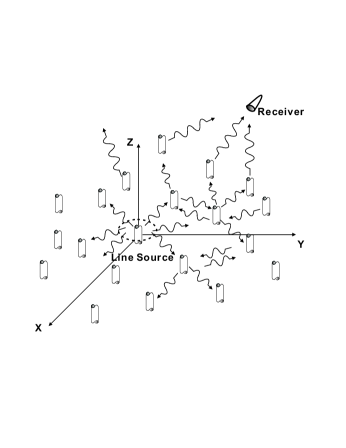
Figure 1: Conceptual layout of the system and the simulation.

II.2 The formulation

Although much of the following materials can be referred to in YLS , we repeat the important parts here for the sake of convenience and completeness.

Upon stimulation, each dipole will radiate EM waves. The radiated waves will then repeatedly interact with the dipoles, forming a process of multiple scattering. The equation of motion for the $i$-th dipole is

$$\frac{d^{2}}{dt^{2}}p_{i}+\omega_{0,i}^{2}p_{i} = \frac{q_{i}^{2}}{m_{i}}E_{z}(\vec{r}_{i})-b_{0,i}\frac{d}{dt}p_{i},$$ (1)

$$\mbox{for}\ i=1,2,\dots,N.$$

where $\omega_{0,i}$ is the resonance (natural) frequency, $p_{i}$, $q_{i}$ and $m_{i}$ the dipole moment, charge and effective mass per unit length of the $i$-th dipole respectively. $E_{z}({\vec{r}_{i}})$ is the total electrical field acting on dipole $p_{i}$, which includes the radiated field from other dipoles and also the directly field from the source. The factor $b_{0,i}$ denotes the damping due to energy loss and radiation, and can be determined by energy conservation. Without energy loss (to such as heat), $b_{0,i}$ can be determined from the balance between the radiative and vibrational energies, and is given asErdogan

$$b_{0,i}=\frac{q_{i}^{2}\omega_{0,i}}{4\epsilon m_{i}c^{2}},$$ (2)

with $\epsilon$ being the constant permittivity and $c$ the speed of light in the medium separately.

Equation (1) is virtually the same as Eq. (1) in Erdogan . The only difference is that in Erdogan , $E_{z}$ is the reflected field at the dipole due to the presence of reflecting surrounding structures, while in the present case the field is from the stimulating source and the radiation from all other dipoles.

The transmitted electrical field from the continuous line source is determined by the Maxwell equationsErdogan

$$\left(\nabla^{2}-\frac{\partial^{2}}{c^{2}\partial t^{2}}\right)G_{0}(\vec{r}-\vec{r}_{s})=-4\mu_{0}\omega^{2}p_{0}\pi\delta^{(2)}(\vec{r}-\vec{r}_{s})e^{-i\omega t},$$ (3)

where $\omega$ is the radiation frequency, and $p_{0}$ is the source strength and is set to be unit. The solution of Eq. (3) is clearly

$$G_{0}(\vec{r}-\vec{r_{s}})=(\mu_{0}\omega^{2}p_{0})i\pi H_{0}^{(1)}(k|\vec{r}-\vec{r}_{s}|)e^{-i\omega t},$$ (4)

with $k=\omega/c$, and $H_{0}^{(1)}$ being the zero-th order Hankel function of the first kind.

Similarly, the radiated field from the $i$-th dipole is given by

$$\left(\nabla^{2}-\frac{\partial^{2}}{c^{2}\partial t^{2}}\right)G_{i}(\vec{r}-\vec{r}_{i})=\mu_{0}\frac{d^{2}}{dt^{2}}p_{i}\delta^{(2)}(\vec{r}-\vec{r}_{i}).$$ (5)

The field arriving at the $i$-th dipole is composed of the direct field from the source and the radiation from all other dipoles, and thus is given as

$$E_{z}(\vec{r}_{i})=G_{0}(\vec{r}_{i}-\vec{r}_{s})+\sum_{j=1,j\neq i}^{N}G_{j}(\vec{r}_{i}-\vec{r}_{j}).$$ (6)

Substituting Eqs. (4), (5), and (6) into Eq. (1), and writing $p_{i}=p_{i}e^{-i\omega t}$, we arrive at

$$(-\omega^{2}+\omega^{2}_{0,i}-i\omega b_{0,i})p_{i}=$$

$$\frac{q_{i}^{2}}{m_{i}}\left[G_{0}(\vec{r}_{i}-\vec{r}_{s})+\sum_{j=1,j\neq i}^{N}\frac{\mu_{0}\omega^{2}}{4}iH_{0}^{(1)}(k|\vec{r}_{i}-\vec{r}_{j}|)p_{i}\right].$$ (7)

This set of linear equations can be solved numerically for $p_{i}$. After $p_{i}$ are obtained, the total field at any space point can be readily calculated from

$$E_{z}(\vec{r})=G_{0}(\vec{r}-\vec{r}_{s})+\sum_{j=1}^{N}G_{j}(\vec{r}-\vec{r}_{j}).$$ (8)

In the standard approach to wave localization, waves are said to be localized when the square modulus of the field $|E(\vec{r})|^{2}$, representing the wave energy, is spatially localized after the trivial cylindrically spreading effect is eliminated. Obviously, this is equivalent to say that the further away is the dipole from the source, the smaller its oscillation amplitude, expected to follow an exponentially decreasing pattern.

To this end, it is instructive to point out that an alternative two dimensional dipole model was devised previously by Rusek and OrlowskiMarian . The authors derived a set of linear algebraic equations, which is similar in form to the above Eq. (6). However, there are some fundamental discrepancies between the two models. In Marian , the interaction between dipoles and the external field is derived by the energy conservation, while in the present case the coupling is determined without ambiguity by the Newton’s second law. The former leads to an undetermined phase factor. According to, e. g. Refs. Erdogan ; ccw , the energy conservation can only give the radiation factor in Eq. (2). We would also like to point out that the set of couple equations in Eq. (7) is similar in spirit to the tight-binding model used to study the electronic localizationAnderson ; Zallen .

There are several ways to introduce randomness to Eq. (7). For example, the disorder may be introduced by randomly varying such properties of individual dipoles as the charge, the mass or the two combined. This is the most common way that the disorder is introduced into the tight-binding model for electronic wavesZallen . In the present study, the disorder is brought in by the random distribution of the dipoles.

For simplicity yet without losing generality, assume that all the dipoles are identical and they are randomly distributed within a square area. The source is located at the center (set to be the origin) of this area. For convenience, we make Eq. (7) non-dimensional by scaling the frequency by the resonance frequency of a single dipole $\omega_{0}$. This will lead to two independent non-dimensional parameters $b=\frac{q^{2}\mu_{0}}{4m}$ and $b_{0}^{\prime}=\frac{\omega}{\omega_{0}}\left(\frac{b_{0}}{\omega_{0}}\right)$. Both parameters may be adjusted in the experiment. For example, the factor $b_{0}$ can be modified by coating layered structures around the dipolesErdogan . Then Eq. (7) becomes simply

$$(-f^{2}+1-ib_{0}^{\prime})p_{i}=$$

$$ibf^{2}\left[p_{0}H_{0}^{(1)}(k|\vec{r}_{i}-\vec{r}_{s}|)+\sum_{j=1,j\neq i}^{N}p_{i}H_{0}^{(1)}(k|\vec{r}_{i}-\vec{r}_{j}|)\right] )$$ (9)

with $f=\frac{\omega}{\omega_{0}}$. Eq. (9) is self-consistent and can be solved numerically for $p_{i}$ and then the total field is obtained through Eqs. (3), (5) and (8).

III The results and discussion

III.1 Two numerical measuring scenarios

In the following computation, we will consider two scenarios. They are illustrated in Fig. 2 with the coordinates being shown. In both cases, the sample takes a fixed rectangular shape of which the size may vary. The dipoles, denoted by the small circles, are placed within the rectangle in a complete randomness. The receiver, denoted by the filled black circle, is placed on the $x$-axis.

In case (A), the sample size is fixed. The receiver is placed along $x$-axis to measure the signal at various positions, yielding the result of the transmission signal versus the distance between the source and the receiver, termed as the travelling distance in the paper. This scenario complies with the original conjecture of observation of localizationLee . In case (B), the receiver is placed at a very small distance outside the sample. While the sample size varies, this method is to measure the transmission through the sample of various sizes, yielding the result of the transmission signal versus the sample size.

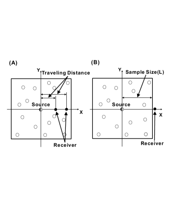
Figure 2: The conceptual layout of the two measuring methods.

III.2 General discussion of localization

Before moving to solve Eq. (7) for the phenomenon of localization of EM waves, we discuss some general properties of wave localization.

The coherence in localization Although some parts of the following discussion has been reported earlier, we repeat here for the sake of convenience and importance. The energy flow of EM waves is $\vec{J}\sim\vec{E}\times\vec{H}$. By invoking the Maxwell equations to relate the electrical and magnetic fields, we can derive that the time averaged energy flow is

$$<\vec{J}>_{t}\equiv\frac{1}{T}\int_{0}^{T}dt\vec{J}\sim|\vec{E}|^{2}\nabla\theta,$$ (10)

where the electrical field is written as $\vec{E}=\vec{e}_{E}|\vec{E}|e^{i\theta}$, with $\vec{e}_{E}$ denoting the direction, $|\vec{E}|$ and $\theta$ being the amplitude and the phase respectively. It is clear from Eq. (10) that when $\theta$ is constant, at least by spatial domains, while $|\vec{E}|\neq 0$, the flow would come to a stop and the energy will be localized or stored in the space. In the localized state, a source can no longer radiate energies. Alternatively, we can write the oscillation of the dipoles as $p_{i}=|p_{i}|e^{i\theta_{i}}$. By studying the square modulus of $p_{i}$ in the form of $|\vec{r}_{i}-\vec{r}_{s}||p_{i}|^{2}$, and its phase $\theta_{i}$, we can also investigate the localization of EM waves. Note here that the factor $|\vec{r}_{i}-\vec{r}_{s}|$ is to eliminate the cylindrical spreading effect in 2D as can be seen from the expansion of the Hankel function $|H_{0}^{(1)}(x)|^{2}\sim\frac{1}{x}$. That the phase $\theta$ is constant implies that a coherence behavior appears in the system, i. e. the localized state is a phase-coherent state, as previously discussedYe2 . It is a unique feature of wave localization, and has also been shown to be related to electronic localization (e. g. Ref. Gurtvitz ).

Spatial behavior of localized waves Following 3D , a general consideration of the spatial behavior of localized waves is possible. Consider a wave transmitted in a random medium. The transport equation for the total energy intensity $I$, i. e. $<|E|^{2}>$, may be intuitively written as

$$\frac{dI}{dx}=-\alpha I,$$ (11)

where $\alpha$ represents decay along the path traversed. After penetrating into the random medium, the wave will be scattered by random inhomogeneities. As a result, the wave coherence starts to decrease, yielding the way to incoherence. Extinction of the coherent intensity $I_{C}$, i. e. $|<E>|^{2}$, is described by

$$\frac{dI_{C}}{dx}=-\gamma I_{C},$$ (12)

with the attenuation constant $\gamma$. Eqs. (11) and (12) lead to the exponential solutions

$$I(x)=I(0)e^{-\alpha x},\ \ \ \mbox{and}\ \ \ I_{C}(x)=I(0)e^{-\gamma x}.$$ (13)

In deriving these equations, the boundary condition was used; it states that $I(0)=I_{C}(0)$ as no scattering has been incurred yet at the interface. According to energy conservation, the incoherent intensity $I_{D}$ (diffusive) is thus

$$I_{D}(x)=I(x)-I_{C}(x).$$ (14)

When there is no absorption, the decay constant $\alpha$ is expected to vanish and the total intensity will then be constant along the propagation path. Then, the coherent energy gradually decreases due to random scattering and transforms to the diffusive energy, while the sum of the two forms of energy remains a constant. This scenario, however, changes when localization occurs. Even without absorption, the total intensity can be localized near the interface due to multiple scattering. When this happens, $\alpha$ does not vanish. The transport of the total intensity may be still described by Eq. (11), and the inverse of $\alpha$ would then refer to the localization length.

The above perceptual description may be illustrated by Fig. 3. Without or with little absorption and with no localization, the energy propagation is anticipated to follow the behavior depicted in (A). When the localization comes in function, the wave will be trapped within an $e$-folding distance from the penetration, as prescribed by (B). In the non-localization case, the diffusive intensity increases steadily as more and more scattering occurs, complying with the Milne diffusion. In the localized state, the diffusion energy increases initially. It will be eventually stopped by the interference of multiple scattering waves. Issues may be raised with respect to whether this apprehended image is supported by actual situations. In the rest, we will inspect this problem.

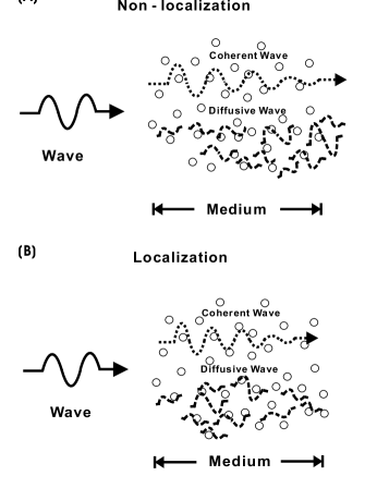
Figure 3: Picturised non-localization and localization effects.

Comparing Fig. 3 (A) and (B), we know that one of the key differences between non-localization and localization features lies in the difference in the behavior of the diffusive waves. However, the eventual task of inferring localization is to find whether the total energy decays with the sample size.

III.3 Numerical results

Unless otherwise noted, the following parameters are used in the numerical simulation: the non-dimensional damping rate, $b_{0}/\omega_{0}=0.001$ and the interaction coupling, $b=0.001$. The filling factor ($\beta$) varies from 2.25 to 25; the filling factor is defined as the number of dipoles per unit area. But without notification, the filling factor is taken as 6.25. The number of random configurations for averaging is taken in such a way that the convergency is assured. In the calculation, we scale all lengths by a length $D$ such that $k_{0}D=1$, and frequency by $\omega_{0}$. In this way, the frequency always enters as $k/k$. We find that all the results shown below are only dependent on parameters $b$, $b_{0}/\omega_{0}$, and the ratio $\omega/\omega_{0}$ or equivalently $k/k_{0}$. Such a simple scaling property may facilitate designing experiments. In the numerical computation, we take $c=1$ for convenience. The total wave at a spatial point is scaled as $T(\vec{r})\equiv E(\vec{r})/E_{0}(\vec{r})$, with $E_{0}$ being the direct wave from the source, so that the trivial geometric spreading effect is naturally removed.

First, we plot the frequency response of the transmission in the scenario (B) of Fig. 2. The results are shown in Fig. 4. Here we see that there is a narrow window within which the transmission is highly inhibited, implying a strong localization effect. It is also clear that when the sample size is increased, the inhibition increases. Comparing the results for the two filling factors, we know that the strong inhibition regime increases with filling factor. In the next computations, we will focus on frequencies within the strong inhibition region.

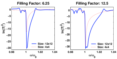
Figure 4: Transmission versus frequency for two filling factors and two sample sizes.

Now we consider the phase and the spatial distribution of energy of the system. To describe the phase behavior of the system, we assign a unit phase vector, $\vec{u}_{i}=\cos\theta_{i}\vec{e}_{x}+\sin\theta_{i}\vec{e}_{y}$ to the oscillation phase $\theta_{i}$ of the dipoles. Here $\vec{e}_{x}$ and $\vec{e}_{y}$ are unit vectors in the $x$ and $y$ directions respectively. These phase vectors are represented by a phase diagram in the $x-y$ plane with the phase vector $\vec{u}_{i}$ being located at the dipole to which the phase $\theta_{i}$ is associated. The results are depicted for three frequencies by Fig. 5.

Here we see clearly shown that for the three frequencies within the strong inhibition region, the energy is spatially confined near the transmitting source, and, as expected, the energy seems to decrease nearly exponentially along any radial direction. Meanwhile, the system reveals an in-phase phenomenon: nearly all the phase vectors of the dipoles point to the same direction, exactly opposite to the phase vector of the source which is denoted by the black arrow. The picture represented by Fig. 5 fully complies with the general description of the coherence in localization stated above.

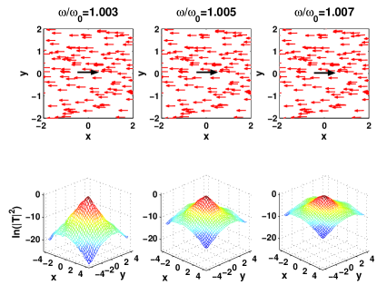
Figure 5: The phase diagram for the two dimensional phase vectors defined in the text; the phase of the source is assumed to be zero. Each vector is located at the site of the dipole; thus the locations of the phase vectors also denote the random distribution of the dipoles. Bottom: The spatial distribution of energy ($\sim|T|^{2}$). Three frequencies are chosen, the sample size is $8\times 8$.

We also note from Fig. 5 that near the sample boundary, the phase vectors start to point to different directions. This is because the numerical simulation is carried out for a finite sample size. For a finite system, the energy can leak out at the boundary, resulting in disorientation of the phase vectors. When enlarging the sample size by adding more dipoles while keeping the averaged distance between dipoles fixed, the area showing the phase coherence will increase accordingly.

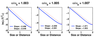
Figure 6: Comparison of the total transmission at three frequencies for the two scenarios shown by Fig. 2. The x-labels ‘Distance’ and ‘Size’ refer to scenario (A) and (B) respectively.

The results of Fig. 5 are encouraging, as they are a strong indication of localization. In the following, we will further explore the features of localization. In Fig. 6, we compare the transmission results for the two scenarios from Fig. 2. Here is shown that although there is a slight difference in the transmitted strength, overall speaking the spatial decay features are nearly identical, signified by the match of the decaying slopes indicated in the figure. Though suspected to be true previously, such a match is important, and to the best of our knowledge this is the first that has been ever shown for EM waves. It supports directly that the scenario (B) can also be used to infer localization effects, facilitating measurements of localization; in the original conjecture, it was scenario (A) that has been suggested for discerning localization. In the rest of simulation, we will adopt scenario (B) in Fig. 2.

The bottom panel of Fig. 6 indicates that the level of spatial localization of energy varies for the three frequencies. To quantify the localization in Fig. 6, we plot the total energy as a function of the sample size. The results are presented by Fig. 7. Here, the numerical data are fitted with the least squares method and the fitted curves are shown by the solid lines; the unnoticeable deviation from the lines reflects the fluctuation due to the random distribution. Two ways of averaging are adopted. One is the traditional way in which the logged total transmission is averaged, while the other is to take log of the averaged total energy. These can be referred to from the y-axis labels. It shows that after removing the spreading factor, the data can be fitted by $e^{-r/\xi}$. From the slope of the solid lines, the localization lengths $\xi$, which are the inverse of the slopes can be estimated. Here is shown that the decaying slopes from the two averaging methods are very close, an encouraging fact. It is also indicated by the decreasing slopes with frequency that the localization effect decreases as the frequency increases.

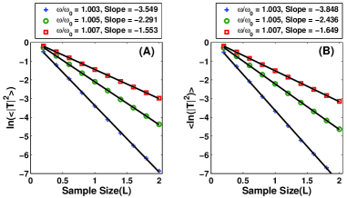
Figure 7: The transmission versus the sample size for three frequencies. The slopes can be used to estimate the localization length.

With the fixed filling factor of 6.25, we have also investigated the spatial variations of the total, coherent and the diffusive energies for three frequencies discussed. The results are presented in Fig. 8. Here we see that the results are in accordance with the previous general consideration of localization. Due to scattering and localization, the coherent waves decrease with the sample size. The diffusive wave increases initially as more and more scattering occurs, then reaches a peak and starts to decay due to the localization effect, in agreement with the description of Fig. 3(B). The results show that in the present system, the diffusive portion in the total energy is much smaller than the coherent portion, indicating that the mean free path is very small. When plotted in the log scale, we have found that the total and coherent energies decays exponentially with the distance, while the diffusive energy increases initially, then starts to decay exponentially. It is worth noting that for the three frequencies considered, the total energy does not reveal any behavior similar to the diffusive waves, in contrast to the previous theoretical conjectureSheng . The theory predicts that the total energy would follow the behavior of diffusive waves until when the sample size is larger than the localization length. One explanation is that in the present system, the scattering is too significant so that the diffusive portion never dominates. A search for the possible match between the simulation and theory in certain conditions is still undergoing.

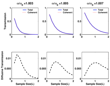
Figure 8: Behaviors of the total, coherent, and the diffusive energies as a function of sample size in the scenario described by Fig. 2(B).

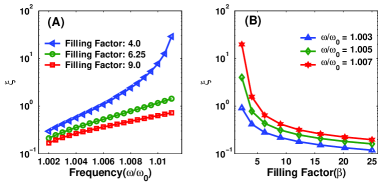
Figure 9: Localization length as a function of (A) frequency and (B) filling factor. The sample size is $8\times 8$ for (A).

In Fig. 9, we plot the localization length versus frequency and filling factor separately. It is shown that with the fixed filling factor, referring to Fig. 9(A), the localization length increases with frequency within the frequency regime considered. With a fixed frequency, the localization length tends to decreases, meaning increasing localization effects, as the filling factor increases.

Fig. 10 shows the transmission versus frequency for various coupling constants and damping rates. From this figure, we observe the following. (1) The increasing coupling strength leads to a wider strong inhibition region, but shallower localization valley. (2) When increasing the coupling strength, a prominent resonance peak appears below the natural frequency $\omega_{0}$. And the peak moves toward lower frequencies as the strength increases, a feature also appears in the acoustic systemYe1 . (3) Overall speaking, the increasing damping rate degrades the localization level, and tends to abolish the resonance peak. Also it seems to widen the strong localization region at the lower frequency side.

IV Summary

In this article, the localization features in a simple electromagnetic system are investigated in detail. Some general properties of the localization phenomenon are elaborated. For certain ranges of frequencies, strongly localized electromagnetic waves have been observed in such a simple but realistic disordered system. It is shown that the localization depends on a number of parameters including frequency, filling factor, and damping rate. The spatial behavior of the total, coherent and diffusive waves is also explored, and found to comply with a physical intuitive picture. A phase diagram characterizing localization is presented, in agreement with previous investigations on other systemsYe2 .

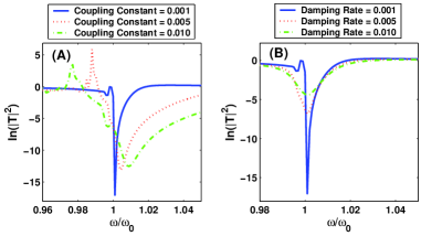
Figure 10: Transmission versus frequency for various coupling strengths and damping factors: (A) various coupling strengths with damping rate 0.001; (B) various damping rates with coupling constant 0.001. The sample size is $4\times 4$.

References

- (1) P. W. Anderson, Phys. Rev. 109, 1492 (1958).
- (2) P. A. Lee and Ramakrishnan, Rev. Mod. Phys. 57, 287 (1985).
- (3) R. Hennino, et. al., Phys. Rev. Lett. 86, 3447 (2001).
- (4) G. I. Barenbatt, M. E. Vinogradov, and S. V. Petrovskii, Oceanology, 35, 202 (1995).
- (5) Z. Q. Zhang, Phys. Rev. B 52, 7960 (1995); S. Wiersma, M. P. van Albada, and A. Lagendijk, Nature, 373, 203 (1997); H. Cao, et. al. Phys. Rev. Lett. 82, 2278 (1999); C. M. Soukoulis, X. Jiang, J. Y. Xu, and H. Cao, Phys. Rev. B 65, 041103 (2002).
- (6) D. J. Thouless, Phys. Rep. 13, 93 (1974).
- (7) S. John, Phys. Today, 44, 52 (1991).
- (8) P. Sheng, Introduction to Wave Scattering, Localization, and Mesoscopic Phenomena (Academic Press, New York, 1995).
- (9) A. Lagendijk and B. A. van Tiggelen, Phys. Rep. 270, 143 (1996).
- (10) B. A. van Tiggelen, in Diffuse Waves in Compex Media (Kluwer Academic Publisher, Netherlands, 1999).
- (11) M. C. W. van Rossum and Th. M. Nieuwenhuizen, Rev. Mod. Phys. 71, 313 (1999)
- (12) M. Janssen, Fluctuations and localization (World Scientific, Singapore, 2001); and references therein.
- (13) C. H. Hodges and J. Woodhouse, J. Acoust. Soc. Am. 74, 894 (1983).
- (14) T. R. Kirkpatrick, Phys. Rev. B 31, 5746 (1985).
- (15) S. He and J. D. Maynard, Phys. Rev. Lett. 57, 3171 (1986).
- (16) C. A. Condat, J. Acoust. Soc. Am. 83, 441 (1988).
- (17) D. Sornette and B. Souillard, Europhys. Letts. 7, 269 (1988).
- (18) A. Z. Genack and N. Garcia, Phys. Rev. Lett. 66, 2064 (1991).
- (19) R. Dalichaouch, J. P. Armstrong, S. Schultz, P. M. Platzman and S. L. McCall, Nature 354, 53 (1991).
- (20) S. L. McCall, P. M. Platzman, R. Dalichaouch, D. Smith, and S. Schultz, Phys. Rev. Lett. 67, 2017 (1991).
- (21) M. Rusek and A. Orlowski, Phys. Rev. E 51, R2763 (1995).
- (22) M. M. Sigalas, C. M. Soukoulis, C.-T. Chan, and D. Turner, Phys. Rev. B 53, 8340 (1996).
- (23) A. A. Asatryan, et al. Phys. Rev. B 57, 13535 (1998).
- (24) Z. Ye and A. Alvarez, Phys. Rev. Lett. 80, 3503 (1998).
- (25) Y. Kuga, A. Ishimaru, J. Opt. Soc. Am. A1, 831 (1984); M. van Albada, A. Lagendijk, Phys. Rev. Lett. 55, 2692 (1985); P. E. Wolf, G. Maret, Phys. Rev. Lett. 55, 2696 (1985); A. Tourin, et al., Phys. Rev. Lett. 79, 3637 (1997); M. Torres, J. P. Adrados, F. R. Montero de Espinosa, Nature 398, 114 (1999).
- (26) D. S. Wiersma, P. Bartolini, A. Lagendijk, and R. Roghini, Nature 390, 671 (1997).
- (27) A. A. Chabanov, M. Stoytchev, and A. Z. Genack, Nature 404, 850 (2000).
- (28) F. Scheffold, R. Lenke, R. Tweer, and G. Maret, Nature 398, 206 (1999); D. Wiersma, et al. Nature, 398, 207 (1999).
- (29) Y.-Y. Chen and Z. Ye, Phys. Rev. E 65, 056612 (2002).
- (30) Z. Ye, S. Li, and X. Sun, Phys. Rev. E 66, 045602(R) (2002).
- (31) T. Erdogan, K. G. Sullivan, and D. G. Hall, J. Opt. Soc. Am. B 10, 391 (1993).
- (32) C.-C. Wang and Z. Ye, Phys. Stat. Sol. (a)174, 527 (1999).
- (33) R. Zallen, The physics of amorphous solids, (John Wiley and Son, New York, 1983).
- (34) E. Hoskinson, and Z. Ye, Phys. Rev. Lett. 83, 2734 (1999).
- (35) S. A. Gurtvitz, Phys. Rev. Lett. 85, 812 (2000); and references therein.
- (36) Z. Ye, H.-R. Hsu, E. Hoskinson, and A. Alvarez, Chin. J. Phys., 37, 343 (1999).