Aspect-ratio dependence of the spin stiffness of a two-dimensional XY model

Abstract

We calculate the superfluid stiffness of 2D lattice hard-core bosons at half-filling (equivalent to the $S=1/2$ XY-model) using the squared winding number quantum Monte Carlo estimator. For $L_{x}\times L_{y}$ lattices with aspect ratio $L_{x}/L_{y}=R$, and $L_{x},L_{y}\to\infty$, we confirm the recent prediction [N. Prokof’ev and B.V. Svistunov, Phys. Rev. B 61, 11282 (2000)] that the finite-temperature stiffness parameters $\rho^{W}_{x}$ and $\rho^{W}_{y}$ determined from the winding number differ from each other and from the true superfluid density $\rho_{s}$. Formally, $\rho^{W}_{y}\rightarrow\rho_{s}$ in the limit in which $L_{x}\rightarrow\infty$ first and then $L_{y}\rightarrow\infty$. In practice we find that $\rho^{W}_{y}$ converges exponentially to $\rho_{s}$ for $R>1$. We also confirm that for 3D systems, $\rho^{W}_{x}=\rho^{W}_{y}=\rho^{W}_{z}=\rho_{s}$ for any $R$. In addition, we determine the Kosterlitz-Thouless transition temperature to be $T_{KT}/J=0.34303(8)$ for the 2D model.

I Introduction

In the usual Kosterlitz-Thouless KTxx description of a 2D superfluid, BishopReppy excitations of bound vortex-antivortex pairs renormalize the superfluid density $\rho_{s}(T)$. Here, $\rho_{s}(T)$ is the coefficient of the square of the gradient of the phase in the free energy expression that governs long-wavelength phase fluctuations. Above a critical temperature $T_{KT}$, the vortex pairs unbind and $\rho_{s}(T)$ drops to zero. The well-known Nelson-Kosterlitz formula, NKxx

$$T_{KT}=\frac{\pi}{2}\ \rho_{s}\,(T_{KT}),$$ (1)

relates $T_{KT}$ to the discontinuity in the superfluid density $\rho_{s}(T_{KT})$ at $T_{KT}$. Using quantum Monte Carlo simulations in a real-space basis, one can calculate a stiffness parameter $\rho^{W}_{\alpha}(T)$, related to $\rho_{s}(T)$, using a squared winding number estimator. stiffness On an $L_{x}\times L_{y}$ torus, we can define two stiffness parameters (or helicity moduli)

$$\rho^{W}_{x}(T) = T\frac{L_{x}}{L_{y}}\langle W^{2}_{x}\rangle,$$ (2)

$$\rho^{W}_{y}(T) = T\frac{L_{y}}{L_{x}}\langle W^{2}_{y}\rangle,$$ (3)

where the integer winding numbers $W_{\alpha}$, $\alpha=x,y$, are defined according to

$$W_{\alpha}=\frac{1}{L_{\alpha}}\int\limits_{0}^{\beta}d\tau J_{\alpha}(\tau),$$ (4)

where $J_{\alpha}$ is the boson current operator and $\beta=1/T$. Typically, systems with aspect ratio $R=L_{x}/L_{y}=1$ have been studied, and in the limit where $L_{x}$ and $L_{y}$ become infinite, one might expect that $\rho^{W}_{\alpha}(T)$ is equal to $\rho_{s}(T)$. However, recently Prokof’ev and Svistunov PSxx have noted that in addition to the Kosterlitz-Thouless vortex-antivortex pairs, topological excitations present for an $L_{x}\times L_{y}$ torus lead to a renormalization of the stiffness parameters. In this case, at finite temperature, even in the limit $L_{x},L_{y}\to\infty$, $\rho^{W}_{x}(T)$ and $\rho^{W}_{y}(T)$ depend upon the aspect ratio and in general do not equal the superfluid density $\rho_{s}(T)$. DJSxx In particular, for $L_{x}=L_{y}$, $\rho^{W}_{x}(T_{KT})/\rho_{s}(T_{KT})\approx 0.9998$. Hence, calculations of $T_{KT}$ utilizing Eq. (1) and assuming $\rho^{W}_{x}=\rho_{s}$ can be expected to be affected by a small (typically negligible) systematic error.

In this paper we present a quantum Monte Carlo study of the aspect ratio dependence of $\rho^{W}_{x}$ and $\rho^{W}_{y}$, organized as follows. In Section II we review the argument of Ref. PSxx, and summarize their conclusions. Section III contains the results of our quantum Monte Carlo study on the $S=1/2$ XY-model. In III.1 we show the dependence of $\rho^{W}_{x}$ and $\rho^{W}_{y}$ on $R$ for 2D and 3D square lattices, and illustrate the need for an accurate, independent estimate of $T_{KT}$ for this model to use as a benchmark. In Section III.2 we use the Weber-Minnhagen RG scaling relation WMxx on systems with $R=1$ and 4 to obtain a very accurate estimate of $T_{KT}$. In Section III.3 we explore a method of calculating $T_{KT}$ using the predicted aspect ratio dependence of $\rho^{W}_{x}$/$\rho^{W}_{y}$, and illustrate the need for precise finite-size scaling of the data in order to obtain satisfactory agreement with the benchmark $T_{KT}$. Once the finite-size scaling behavior of $\rho^{W}_{x}$/$\rho^{W}_{y}$ is understood, it is straightforward to confirm the conclusions of Ref. PSxx, using our data.

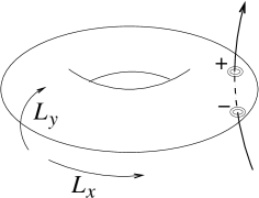
Figure 1: A 2D superfluid with vortex excitations. The vortices are located at the points where the flux tube of circulation pierces the surface of the torus ($+$ and $-$ refer to a vortex and an antivortex).

II Stiffness Parameters

Consider the $L_{x}\times L_{y}$ torus shown in Fig. 1. Imagine that its surface is coated with a 2D superfluid and that a tube of quantized circulation $h/m$ penetrates the torus as shown in Fig. 1. There is an antivortex in the superfluid layer at the point where this flux tube passes into the torus, and a vortex at the point where it leaves the surface. These excitations are the Kosterlitz-Thouless vortex-antivortex pairs. On a finite torus one can also envision a situation in which the flux tube moves through the cross-section and into the center of the torus as illustrated in Fig. 2. In this case a single unit of quantized flux has entered the torus (Fig. 2(c)), and the excitation energy is

$$\epsilon_{x}=\frac{\rho_{s}(T)}{2}\ \left(\frac{2\pi}{L_{x}}\right)^{2}L_{x}\,L_{y}=2\pi^{2}\rho_{s}(T)\ \frac{L_{y}}{L_{x}}.$$ (5)

Here, $\rho_{s}(T)$ is the usual Kosterlitz-Thouless superfluid density which is renormalized by the vortex-antivortex pairs. Naturally, there are excitations with energy $\epsilon_{x}\ell^{2}$ associated with flux tubes containing $\ell$ quanta. Similarly, there are excitations associated with a flux tube which threads around the inside of the torus along the $L_{x}$ direction. The energies of these excitations will vary as $L_{x}/L_{y}$.

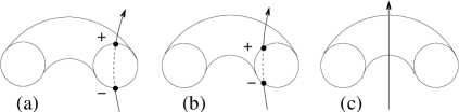
Figure 2: Cross section of a torus, showing a flux line as it passes through to the center of the superfluid. In (a) the vortex-antivortex pair is maximally separated, in (b) the pair moves closer together and in (c) the pair has annihilated each other. The tube of quantized flux remains.

At finite temperatures, the phase stiffness parameters $\rho^{W}_{x}$ and $\rho^{W}_{y}$ are affected by the vortex excitations. In the usual way, the stiffness is determined from the change in the free energy associated with an infinitesimal flux $\phi$ threading the torus. With $\phi$ in the direction of the flux tube in Fig. 1, one obtains $\rho^{W}_{x}(T)$ from

$$\Delta F_{x}=\frac{1}{2}\ \rho^{W}_{x}(T)\ \frac{L_{y}}{L_{x}}\ \theta^{2},$$ (6)

with $\theta=2\pi\phi/(h/m)$. As discussed in Ref. PSxx, , a calculation of $\Delta F$ gives

$$\rho^{W}_{x}(T)=\rho_{s}(T)\ \left(1-\frac{4\pi^{2}\rho_{s}(T)}{T}\ \frac{L_{y}}{L_{x}}\langle\ell^{2}\rangle_{x}\right),$$ (7)

where $\ell$ is the number of quanta in the flux tube, and

$$\langle\ell^{2}\rangle_{x}=\frac{\sum\limits_{\ell}\ e^{-\left(\frac{\epsilon_{x}}{T}\right)\ell^{2}}\ell^{2}}{\sum\limits_{\ell}\ e^{-\left(\frac{\epsilon_{x}}{T}\right)\ell^{2}}}.$$ (8)

The stiffness in the y-direction is obtained by replacing $L_{y}/L_{x}$ by $L_{x}/L_{y}$ in Eqs. (7) and (8).

If one lets $L_{x}$ go towards infinity, keeping $L_{y}$ finite,

$$\langle\ell^{2}\rangle_{x}\cong\frac{(L_{x}/L_{y})\,T}{4\pi^{2}\rho_{s}(T)},$$ (9)

so that $\rho^{W}_{x}$ goes to zero as expected for a 1D system at finite $T$. Alternatively, if the aspect ratio is such that $L_{x}$ is large compared to $L_{y}$, then

$$\rho^{W}_{y}(T)=\rho_{s}(T)\ \left(1-\frac{8\pi^{2}\rho_{s}(T)}{T}\ \frac{L_{x}}{L_{y}}\ e^{-2\pi^{2}\frac{\rho_{s}(T)}{T}\ \frac{L_{x}}{L_{y}}}\right),$$ (10)

and the difference between $\rho^{W}_{y}(T)$ and $\rho_{s}(T)$ vanishes exponentially as $L_{x}/L_{y}$ increases. Finally, in 3D the additional factor of $L_{z}$ which occurs in Eq. (7) assures the convergence of $\rho^{W}_{x}$ to $\rho_{s}$ for all $R$ as the size of the system goes to infinity.

In the 2D superfluid, the jump in the stiffnesses at the Kosterlitz-Thouless temperature also clearly depends on the aspect ratio. At $T_{KT}$, using the Nelson-Kosterlitz relation (1), one has PSxx

$$\rho^{W}_{x}(T_{KT})=\rho_{s}(T_{KT})\ \ \left(1-8\pi\ \frac{L_{y}}{L_{x}}\ \langle\ell^{2}\rangle_{x}\right),$$ (11)

with

$$\langle\ell^{2}\rangle_{x}=\frac{\sum\ell^{2}e^{-4\pi\frac{L_{y}}{L_{x}}\ell^{2}}}{\sum e^{-4\pi\frac{L_{y}}{L_{x}}\ell^{2}}}.$$ (12)

In a similar way, $\rho^{W}_{y}(T_{KT})$ and $\langle\ell^{2}\rangle_{y}$ are obtained by replacing ${L_{y}}/{L_{x}}$ by ${L_{x}}/{L_{y}}$ in the above two equations. Hence, one can determine the ratios $\rho^{W}_{x}/\rho_{s}$ and $\rho^{W}_{y}/\rho_{s}$ at $T_{KT}$ by evaluating the sums for $\langle\ell^{2}\rangle_{x}$ and $\langle\ell^{2}\rangle_{y}$. Table 1 shows the result of this calculation for various aspect ratios.

Table 1: Stiffness parameter ratios at $T_{KT}$, for different aspect ratios $R=L_{x}/L_{y}$. The entry * was evaluated explicitly, Berndt while the remaining entries were evaluated to arbitrary numerical accuracy using Waterloo’s Maple V software.

$R$		${\rho^{W}_{x}}/{\rho_{s}}$		${\rho^{W}_{y}}/{\rho_{s}}$
$1$		$0.9998247$		$0.9998247$
$2$		$0.9532407$		$1-1.222613\times 10^{-9}$
$3$		$0.7533903$		$1-6.395505\times 10^{-15}$
$4$		$1/2^{*}$		$1-2.973776\times 10^{-20}$
$5$		$0.2977676$		$1-1.296322\times 10^{-25}$
$6$		$0.1663429$		$1-5.424861\times 10^{-31}$
$7$		$0.0893401$		$1-2.207141\times 10^{-36}$
$8$		$0.0467593$		$1-8.796634\times 10^{-42}$

III Monte Carlo Calculations

In order to study this aspect ratio dependence of $\rho^{W}_{x}$ and $\rho^{W}_{y}$ we employ a model of a two dimensional superfluid using a hard-core boson Hamiltonian at half filling, which is equivalent to the quantum $S={1}/{2}$ XY model defined by

$$H=-J\sum_{\langle i,j\rangle}\left[{S_{i}^{x}S_{j}^{x}+S_{i}^{y}S_{j}^{y}}\right].$$ (13)

Here $S_{i}^{x}$ and $S_{i}^{y}$ are the $x$ and $y$ components of a spin ${1}/{2}$ operator at site $i$, and the sum is carried out over all nearest-neighbor spin pairs $\langle i,j\rangle$. This model is known to have a Kosterlitz-Thouless type transition from previous Monte Carlo simulations carried out on square lattices. AWS1 ; Harada We carry out simulations using the stochastic series expansion (SSE) quantum Monte Carlo method, AWS3 that has previously been applied to this and other spin and boson models. The basis of the SSE method is importance sampling of the power series expansion of the partition function:

$$Z=Tr\{e^{-\beta H}\}=\sum_{\gamma}\sum_{n=0}^{\infty}\frac{(-\beta)^{n}}{n!}\langle{\gamma|H^{n}|\gamma}\rangle,$$ (14)

where $\beta=1/T$ is the inverse temperature and the trace has been written as a sum over diagonal matrix elements in a basis $\{|\gamma\rangle\}$. In our case this is the standard basis of $z$ spin quantization. In the simulations we employ an efficient cluster-type method for sampling the terms of the expansion, called the directed-loop algorithm, AWS3 which in the present case of zero field is similar to loop algorithms previously employed on the spin ${1}/{2}$ XY model. Harada Note that all contributing expansion-orders $n$ in (14) are sampled, and all results are exact within statistical errors.

A direct estimator for the superfluid (spin) stiffnesses is identified in the SSE quantum Monte Carlo in a way analogous to world-line quantum Monte Carlo methods. stiffness ; Harada Starting from the definition Eq. (6) and taking the second derivative of the free energy (per spin) with respect to a twist $\theta$ in the boundary condition will lead to the expressions given in Eq. (2) and (3). The winding number in these equations is now a measure of the net spin currents flowing around the periodic system, $W_{\alpha}=(N_{\alpha}^{R}-N_{\alpha}^{L})/L_{\alpha}$, ($\alpha=x,y$) where $N_{\alpha}^{R,L}$ is the number of operators transporting spin to the “right” or “left” along the $\alpha$ direction in the SSE configuration.

III.1 Spin Stiffness in 2D and 3D

Figure 3: The spin stiffness order parameter Eqs. (2),(3) calculated for a (a) 16$\times$16$\times$64 system and a (b) 64$\times$16 system. The long lattice direction is $z$ and $x$, respectively. The slight deviation of $\rho^{W}_{z}(T)$ around $T/J\approx 1.0$ in (a) disappears in the limit of large system size. The thick dashed line in (b) represents the equation $\rho^{W}_{\alpha}={2T}/{\pi J}$, and the thin vertical dotted line marks the corresponding estimate of $T_{KT}/J$.

In order to test the predictions of Prokof’ev and Svistunov, PSxx we carried out a series of simulations using the Hamiltonian, Eq. (13), for systems with various aspect ratios in two and three dimensions. In general our calculations confirm the predictions of Ref. PSxx, , namely that in the 3D system, the difference between the components of $\rho^{W}_{\alpha}(T)$ ($\alpha=x,y,z$) vanishes exponentially, while in 2D, $\rho^{W}_{x}(T)$ can differ significantly from $\rho^{W}_{y}(T)$ depending on the value of the aspect ratio $R$. Specific examples are illustrated in Fig. 3. As we see in Fig. 3(a), in the 3D case, for $L_{x}/L_{y}=1$ and $L_{z}/L_{y}=4$ the three different spin stiffness parameters converge to one value. In contrast, for the 2D case (Fig. 3(b)), with $R=L_{x}/L_{y}=4$ the spin stiffness in the long direction is significantly less that the spin stiffness in the short direction for a large range of $T$. As we will see below, in 2D $\rho^{W}_{x}(T)$ does not converge to $\rho^{W}_{y}(T)$ in this temperature range even in the limit of large system sizes (over $6.5\times 10^{4}$ spins).

A rough estimate of $T_{KT}$ and the ratio $\rho^{W}_{x}(T_{KT})/\rho^{W}_{y}(T_{KT})$ can be obtained from Fig. 3(b), by drawing a straight line $\rho^{W}_{\alpha}={2T}/{\pi J}$. The point where this line intersects $\rho^{W}_{y}\approx\rho_{s}$ is a finite-size measurement of $T_{KT}/J$, and the ratio $\rho^{W}_{x}/\rho^{W}_{y}$ at this $T$ can be compared to the value 1/2 from Table 1 (which we expect to be exact in the limit of infinite system size). It is clear from this simple demonstration that if one wishes to study the spin stiffness dependence on $R$ in detail, an accurate independent estimate of $T_{KT}$ will facilitate quantitative comparisons of $\rho^{W}_{x}/\rho^{W}_{y}$ with the entries in Table 1. The next section of this paper is therefore dedicated to the measurement of $T_{KT}$.

III.2 Weber-MinnhagenWMxx determination of $T_{KT}$

We now give details on the independent estimate for $T_{KT}$ which will be used as a benchmark for $T_{KT}(L\rightarrow\infty)$ in the discussion to follow. Our approach follows that of Harada and Kawashima, Harada who carried out simulations of the quantum $S={1}/{2}$ XY model on nine square lattices of size $L=8$ to 128. Their analysis found a $T_{KT}=0.3427(2)J$, based on a Weber-Minnhagen WMxx scaling fit for the system size dependence of the spin stiffness. Specifically, this scaling form states that as $T\rightarrow T_{KT}^{-}$,

$$\rho_{s}(L)=\rho_{s}(\infty)\left[{1+\frac{1}{2}\frac{1}{\ln(L)+C)}}\right],$$ (15)

where $\rho_{s}(L)$ now represents the spin stiffness at a finite lattice with a linear size of $L$ spins, $\rho_{s}(\infty)$ is given by Eq. (1), and $C$ is some unknown constant. One can also reformulate Eq. (15) in the linear form,

$$Y(L)=\pi\ln(L)+C,$$ (16)

where

$$Y(L)=\left[{\frac{\rho^{W}_{y}(L)}{F(R)}\frac{1}{T}-\frac{2}{\pi}}\right]^{-1},$$ (17)

and $C$ has been re-scaled to absorb some simple constants. The factor $F(R)$ has been included in order to correct $\rho_{y}^{W}$ according to $\rho_{s}=\rho^{W}_{y}/F(R)$ for square systems, where $F(1)=0.9998247$ from Table 1.

Figure 4: $\chi^{2}$ values (per degree of freedom) for $R=1$, lattice sequence $L=16,24,32,40,48,56,64,72,96,128$ and $R=4$, $L_{y}=16,20,24,32,40,48,56,64$.

In order to obtain results on a dense temperature grid, we did an extensive series of simulated tempering MARxx simulations within a $T$ range centered about the approximate $T_{KT}\approx 0.343J$. Harada Fits to Eq. (16), adjusting $C$ only, should have a minimum in $\chi^{2}$ at $T_{KT}/J$. This is illustrated in Fig. 4. In general, we find that the qualities of the $\chi^{2}$ curves can differ significantly depending on the “lattice sequence” included in the fit. An acceptable lattice sequence should be one that produces a $\chi^{2}$ minimum of approximately unity. We therefore systematically eliminate the smallest $L_{y}$ values from the lattice sequence until $\chi^{2}_{min}\approx 1$. With our tempering data, this occurs when the largest excluded data point is $L_{y}=8$, however to be cautious we also excluded $L_{y}=12$. Qualitatively, the shift in $\chi^{2}_{min}$ is very small ($\Delta T/J<0.0001$) when $L_{y}>16$ points are excluded from the data set, which in part is due to the trivial statistical systematic shift resulting from the elimination of data points from the fit. Finally, the $\chi^{2}$ curves have little quantitative dependence on the maximum $L_{y}$ included, as long as this $L_{y}\geq 64$.

Figure 5: Simulated tempering data for $\rho^{W}_{y}$, where each data point represents $2\times 10^{7}$ Monte Carlo production steps. Statistical errors are at most of the order of the symbol sizes. The star on the vertical axis is $\rho_{y}^{W}(L_{y}\rightarrow\infty)$ determined from $T_{KT}=0.343J$ using Eq. (1). Inset: $\rho^{W}_{y}$ data scaled to the form Eq. (16). Data included in the $\chi^{2}$ fit is plotted with solid symbols, and data for smaller system sizes that was omitted from the $\chi^{2}$ fit is plotted with open symbols. The solid lines have constant slopes of $\pi$.

Using the scaling form Eq. (16) with the data illustrated in Fig. 5, we obtain three estimates for $T_{KT}(\infty)$: for (i) $R=4$, using $F(R)=1$, (ii) $R=1$, with the approximation $F(R)=1$, and (iii) $R=1$, with the correct factor $F(R)=0.9998247$ from Table 1. The corresponding results for the transition temperatures are $T^{(i)}_{KT}/J=0.34302\pm 1.4\times 10^{-4}$, $T^{(ii)}_{KT}/J=0.34302\pm 0.9\times 10^{-4}$ and $T^{(iii)}_{KT}/J=0.34304\pm 1.0\times 10^{-4}$, respectively, where quoted errors are one standard deviation. From this, we see that $T^{(i)}_{KT}=T^{(ii)}_{KT}=T^{(iii)}_{KT}$ to within our statistical error. To obtain a more accurate estimate for the transition temperature, we may also perform a weighted average of our values for $T^{i}_{KT}$ and $T^{iii}_{KT}$, to get $T_{KT}/J=0.34303(8)$. This value agrees to the previousHarada most accurate $T_{KT}=0.3427(2)J$ to within two standard deviations.

The Monte Carlo data and the $\chi^{2}$ fit at our estimated $T_{KT}$ are shown in Fig. 5. As evident there, the unscaled $\rho_{y}^{W}$ data at $T/J=0.34303$ do not clearly approach the infinite size limit determined with Eq. (1). However, when properly scaled according to Eq. (17), $Y(L)$ does become linear according to the expected form Eq. (16) (Fig. 5 inset).

III.3 The Spin Stiffness Ratio $\rho_{x}^{W}/\rho_{y}^{W}$ at $T_{KT}$

In this section we study the aspect ratio dependence of the spin stiffness in more general terms, and outline a procedure for calculating $T_{KT}$ using $\rho_{x}^{W}/\rho_{y}^{W}$ and the results of Table 1. Our aim here is not to obtain a more precise value for $T_{KT}$, but to test how closely the predicted values for the ratios can be observed in practice.

To begin, we collected detailed data for $\rho^{W}_{x}(T)$ and $\rho^{W}_{y}(T)$ for 20 to 24 values of $T/J$ between 0.325 and 0.375. Simulations produced between $1\times 10^{6}$ and $5\times 10^{6}$ Monte Carlo steps at each $T$ (depending on system size and statistical error bars), except for the very largest systems which had an order of magnitude less Monte Carlo steps. System aspect ratios included were $R=$1,2 and 4. Continuous data over $T$ was obtained by fitting third-order polynomial curves.

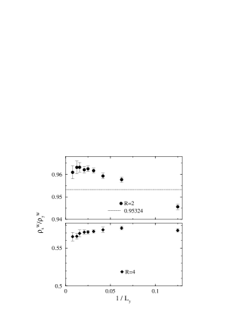
Figure 6: The spin stiffness ratios for $R=2$ and $R=4$ at $T/J=0.34303$. At $T=T_{KT}$ and $L_{x},L_{y}\rightarrow\infty$, the values are expected to approach $\rho_{x}^{W}/\rho_{y}^{W}=0.95324$ and $1/2$, respectively.

Fig. 6 shows the spin stiffness ratios $\rho_{x}^{W}/\rho_{y}^{W}$ calculated with this data, at $T_{KT}/J=0.34303$, as was determined independently in Section III.2 above. As evident in the figure, this type of simple analysis is not very satisfying, as the spin stiffness ratios do not obviously approach the values expected from Table 1. Clearly there are significant finite-size effects at play, as seen previously in the Weber-Minnhagen scaling analysis of Section III.2 (Fig. 5). One way to quantitatively account for the scaling effects in our $\rho_{x}^{W}/\rho_{y}^{W}$ will now be outlined. To do so, we define a new measurement technique which can be used to estimate the Kosterlitz-Thouless transition temperature: namely, $T_{KT}$ is defined as the temperature at which the ratio $\rho^{W}_{x}/\rho_{s}$ (in practice $\rho^{W}_{x}/\rho^{W}_{y}$), passes through the corresponding value in column 2 of Table 1 (for $R=$2 and 4 only). Additionally, for the purposes of comparison, $T_{KT}$ can be obtained by calculating the crossing of Eq. (1) with the $\rho^{W}_{y}(T)$ data for each system size $L_{x}\times L_{y}$. The results of these two procedures are summarized in Fig. 7.

Figure 7: The Kosterlitz-Thouless transition temperature calculated with the Nelson-Kosterlitz formula (NK, Eq. (1)), and with the spin stiffness aspect ratios (PS, Table 1), as a function of inverse linear system size. The infinite size limit is $T_{KT}\approx 0.343J$ (see Section III.2 of text) and is plotted as a star on the vertical axis.

Several interesting observations can be made from this figure. First, if one were only to consider smaller system sizes ($L_{y}<64$), the data would appear to consistently approach an infinite size limit of $T_{KT}/J\approx 0.35$. However, at $L_{y}\approx 64$ we observe that all of the data sets in Fig. 7 undergo subtle changes in slope that could indeed suggest a significantly lower value for $T_{KT}$ in the infinite size limit. Note in particular the change in the sign of the slope for the PS, $R=2$ line at $L_{y}\approx 64$. Without any a priori knowledge of the form of the scaling laws for the curves in Fig. 7, it would be difficult to conclude whether they approach the Kosterlitz-Thouless temperature of $T_{KT}\approx 0.343J$ calculated in Section III.2, and in Ref. Harada, , illustrated on the vertical axis of Fig. 7.

Figure 8: The Kosterlitz-Thouless transition temperatures scaled according to Eq. (19). In (a), the $T_{KT}$ data for $R=4$ becomes approximately linear (excluding the smallest system size, $L_{y}=8$) for $L_{0}\approx 0.01$. In (b), all $T_{KT}$ curves become approximately linear for $L_{0}$ in a narrow range around 0.3. Straight lines are included as guides for the eye. The infinite size limit is $T_{KT}=0.343J$ (see Section III.2 of text) and is plotted as a star on the vertical axis.

We now consider a scaling law for $T_{KT}$ that arises from the Kosterlitz RG scaling equations.KosterlitzRG As discussed in Ref. KosterlitzRG, , the functional form of the correlation length suggests that, as $T\rightarrow T_{KT}$, $\xi$ diverges according to

$$\xi\sim\textrm{exp}(bt^{-1/2}),$$ (18)

where $t=(T-T_{KT})/T_{KT}>0$ and $b$ is a constant. If we identify $\xi=L/L_{0}$ ($L_{0}$ some microscopic length), and $T=T_{KT}(L)$, then we can write the system size-dependent Kosterlitz-Thouless transition temperature in terms of $L/L_{0}$ as

$$T_{KT}(L)=T_{KT}(\infty)\left[{1+\frac{b^{2}}{\ln^{2}(L/L_{0})}}\right].$$ (19)

Fig. 8 illustrates the $T_{KT}(L)$ data of Fig. 7, re-scaled to the form of Eq. (19), for some value of $L_{0}$ which approximately linearizes the data. As this figure shows, by choosing appropriate values for $L_{0}$ it is possible to obtain linear fits to Eq. (19) for all data sets save one. The exception is the spin stiffness aspect ratio crossing for $R=2$ (PS, $R=2$ in Figs. 7 and 8). In this case, the change in slope of the data set at $L_{y}\approx 64$ precludes any direct fitting to the scaled form Eq. (19). However, the data for $L_{y}>64$ show rough evidence of this scaling trend, and it is therefore very likely that additional data for $L_{y}>128$ would approach this $T_{KT}(\infty)$ consistently.

As Fig. 8 shows, the approximate intercept of these scaled data sets are in good agreement with the value of $T_{KT}(\infty)$ calculated in Section III.2 using the Weber-MinnhagenWMxx scaling form for the spin stiffness. In particular, the consistency of the intercept for the data set PS, $R=4$, adds confidence to the assertion that $T_{KT}(L)$ calculated using the spin stiffness aspect ratios is a good estimator for the Kosterlitz-Thouless transition temperature, consistent with $T_{KT}$ calculated using other methods. Thus the entries in Table 1 indeed appear to be accurate. Clearly, however, our value of $T_{KT}/J=0.34303(8)$ obtained from the Weber-Minnhagen scaling is the most accurate because it is based on a one-parameter fit, Eq. (16), as opposed to the two-parameter fit, Eq. (19).

IV Conclusions

In conclusion, we have confirmed the prediction of Prokof’ev and Svistunov PSxx that in 2D the squared winding-number estimates of the finite-temperature spin stiffnesses $\rho^{W}_{x}$ and $\rho^{W}_{y}$ differ from each other for $R\neq 1$, while in 3D systems $\rho^{W}_{x}=\rho^{W}_{y}=\rho^{W}_{z}$ for any $R$. In 2D we also find that $\rho^{W}_{y}$ approaches the Nelson-Kosterlitz superfluid density $\rho_{s}$ exponentially for $R>1$ as $L_{x},L_{y}\rightarrow\infty$, whereas $\rho^{W}_{x}$ approaches zero as $R\to\infty$ exactly as predicted.

As illustrated in Fig. 8, the $T_{KT}$ predicted from the ratios $\rho^{W}_{x}/\rho^{W}_{y}$ approach the $T_{KT}$ predicted using other methods, substantiating the validity of the results listed in Table 1. Neglecting the small differences between $\rho_{s}$ and $\rho^{W}_{x,y}$ on 2D $L\times L$ ($R=1$) lattices is insignificant compared to presently typical statistical uncertainties. However, with any further increase in accuracy relative to that achieved in the data presented here, the effect has to be taken into account in order to avoid a systematic error.

- (1) J. M. Kosterlitz and D. J. Thouless, J. Phys. C 6, 1181 (1973).
- (2) D. J. Bishop and J. D. Reppy, Phys. Rev. Lett. 40, 1727 (1978).
- (3) D. R. Nelson and J. M. Kosterlitz, Phys. Rev. Lett. 39, 1201 (1977).
- (4) E. L. Pollock and D. M. Ceperley, Phys. Rev. B 36, 8343 (1987).
- (5) N. V. Prokof’ev and B. V. Svistunov, Phys. Rev. B 61, 11282 (2000).
- (6) The limiting case, where first, then , was also established earlier by D.J. Scalapino, S. R. White, and S. Zhang, Phys. Rev. B 47, 7995 (1993).
- (7) H. Weber and P. Minnhagen, Phys. Rev. B 37, 5986 (1987).
- (8) In the case , the sum Eq. (12) can be written in terms of Ramanujan’s theta function. It was evaluated explicitly by Ramanujan in B. C. Berndt, “Ramanujan’s Notebooks, Part III”, pp. 102-104, Springer-Verlag, New York (1991).
- (9) H.-Q Ding and M.S. Makivic, Phys. Rev. B 42, 6827 (1990); M.S. Makivic and H.-Q Ding, Phys. Rev. B 43, 3562 (1991); A. W. Sandvik and C. J. Hamer, Phys. Rev. B 60, 6588 (1999).
- (10) K. Harada and N. Kawashima, J. Phys. Soc. Jpn. 67, 2768 (1998).
- (11) A. W. Sandvik, Phys. Rev. B 56, 11678 (1997); O. F. Syljuåsen and A. W. Sandvik, Phys. Rev. E 66 046701 (2002).
- (12) E. Marinari and G. Parisi, Europhys Lett. 19, 451 (1992).
- (13) J. M. Kosterlitz, J. Phys. C 7, 1046 (1974).