Collapses and explosions in self-gravitating systems

Abstract

Collapse and reverse to collapse explosion transition in self-gravitating systems are studied by molecular dynamics simulations. A microcanonical ensemble of point particles confined to a spherical box is considered; the particles interact via an attractive soft Coulomb potential. It is observed that the collapse in the particle system indeed takes place when the energy of the uniform state is put near or below the metastability-instability threshold (collapse energy), predicted by the mean-field theory. Similarly, the explosion in the particle system occurs when the energy of the core-halo state is increased above the explosion energy, where according to the mean field predictions the core-halo state becomes unstable. For a system consisting of 125 – 500 particles, the collapse takes about $10^{5}$ single particle crossing times to complete, while a typical explosion is by an order of magnitude faster. A finite lifetime of metastable states is observed. It is also found that the mean-field description of the uniform and the core-halo states is exact within the statistical uncertainty of the molecular dynamics data.

I Introduction

Systems of particles interacting via a potential with attractive nonintegrable large $r$ asymptotics, $U(r)\sim r^{-\alpha}$, $0<\alpha<3$, and sufficiently short-range small $r$ regularization exhibit gravitational phase transition between a relatively uniform high energy state and a low-energy state with a core-halo structure pr ; ki2 ; ch1 ; usg ; dv ; ch ; chs ; chi . Extensive mean-field (MF) studies of the equilibrium properties of such systems pr ; ki2 ; ch1 ; usg ; dv ; ch ; chs ; chi revealed that in a microcanonical ensemble during such a transition entropy has to undergo a discontinuous jump from a state that just ceases to be a local entropy maximum to a state with the same energy but different temperature, which is the global entropy maximum. Due to the long-range nature of gravitational interaction, the MF studies are believed to provide asymptotically (in the infinite system limit) exact information about the density and the velocity distributions and other thermodynamical parameters of the uniform state. The applicability of the MF theory to the description of the core-halo state is less obvious as the properties of a core are controlled by the short-range asymptotics of the potential.

Relatively little is known about how such a transition actually occurs, however. Youngkins and Miller bm2 performed a Molecular Dynamics (MD) study of a one-dimensional system consisting of concentric spherical shells. Their main emphasis was to check the MF description of the stable and metastable states rather than to study the dynamics of the phase transition itself. Cerruti-Sola, Cipriani, and Pettini pet studied the phase diagram of a more realistic 3-dimensional particle system by using Monte Carlo and MD methods. Their studies again focused on the equilibrium properties of the system rather than on the dynamics of the transitions. In addition, their general conclusions about the second order of the gravitational phase transition apparently contradict the MF results ki2 ; usg ; dv ; chi .

Here, we attempt to resolve this contradiction. A MF description of the dynamics of collapse in ensembles of self-gravitating Brownian particles with a bare $1/r$ interaction based on a Smoluchowski equation was developed by Chavanis et al chs . It predicts a self-similar evolution of the central part of density distribution to a finite-time singularity. However, the precise nature of the random force and friction terms in the corresponding Fokker-Plank equation as well as the applicability of the overdamped limit used to reduce the Fokker-Plank equation to the Smoluchowski equation are not entirely understood. A more rigorous approach based on the Fokker-Plank equation with Landau collision integral was used by Lancellotti and Kiessling ki3 to prove a scaling property of the central part of the density profile. The model considered there allows the particles to escape to infinity and therefore does not have an equilibrium or even a metastable state.

There exists a vast amount of literature on cosmologically- and astrophysically- motivated studies of the temporal evolution of naturally occurring self-gravitating systems (see, e.g., Ref. cos and references therein). The selection of systems and their initial and final conditions made in such studies are typically astrophysically-motivated; the considered systems are often too complex to make a general conclusions about the phase diagrams and phase transitions in such systems.

In this paper we present MD studies of gravitational collapse, and reverse to collapse, i.e., explosion, transitions in a microcanonical ensemble of self-attracting particles. Besides their pure statistical mechanical implications, these studies represent our attempt to bridge a gap between the usually complicated MD and hydrodynamic simulations of the realistic astrophysical systems and the MF analysis of the phase diagram of simple self-gravitating models.

A system with soft Coulomb potential $-(r^{2}+r_{0}^{2})^{-1/2}$ is considered. Such systems are have been studied using both MF theory (see, e.g., Refs. usg ; chi ) and simulations pet . We chose the microcanonical ensemble as the most fundamental one for the long-range interacting systems. It has to be noted that the considered system is strongly ensemble-dependent: While the nature of the uniform state is the same in both microcanonical and canonical ensembles (apart form the difference in their stability range), the core-halo states and the collapse itself in these ensembles have very little in common with each other dv ; chs .

A MF phase diagram of the considered self-attracting microcanonical system is presented in Fig. (1) usg ; chi .

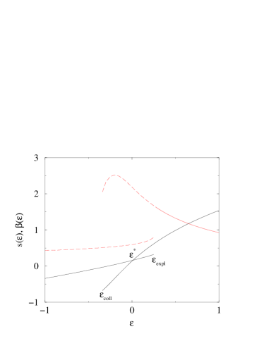
Figure 1: Plots of entropy $s(\epsilon)$ (solid line) and inverse temperature $\beta(\epsilon)=ds/d\epsilon$ (dashed line) vs. energy $\epsilon$ for a system with a gravitational phase transition and a short-range cutoff.

High- and low-energy branches terminating at the energies $\epsilon_{coll}$ and $\epsilon_{expl}$ correspond to the uniform and core-halo states. The energy $\epsilon^{*}$ where the entropies of the core-halo and uniform states are equal is the energy of the true phase transition; the uniform and the core-halo states are metastable in the energy intervals $(\epsilon_{coll},\epsilon^{*})$ and $(\epsilon^{*},\epsilon_{expl})$, respectively. However, for the phase transition to occur at or near $\epsilon^{*}$, a macroscopic-scale fluctuation with prohibitively low entropy is required. Consequently, the metastable branches are stable everywhere except at the vicinity of $\Delta\epsilon\sim N^{-2/3}$ of their end-points $\epsilon_{coll}$ and $\epsilon_{expl}$ ka2 ; chi , where $N$ is the number of particles in the system. Hence it is natural to assume that once the energy of the system in the uniform state is set sufficiently near above or below $\epsilon_{coll}$, the system will undergo a collapse to a core-halo state with the same energy and higher entropy. Similarly, if the energy of the core-halo system is set sufficiently near below or above $\epsilon_{expl}$, the system will undergo an explosion bringing it to a uniform state with the same energy and higher entropy. Our goal here is to study if and how such collapse and explosion proceed in a realistic three-dimensional N-particle dynamical system.

The paper is organized as follows. In the next section we formally introduce the system, outline the MF analysis and describe the MD setup. Then, we present the simulation results for the equilibrium uniform and core-halo states and compare them to the MF predictions. After that we describe and interpret the observed dynamics of the collapse and the explosion transitions. A discussion of the obtained results concludes the paper.

II simulation

We consider a system consisting of $N$ identical particles of unit mass confined to a spherical container of radius $R$ with reflecting walls. The particles interact via the attractive soft Coulomb pair potential $-(r^{2}+r_{0}^{2})^{-1/2}$. Using a traditional convention for self-gravitating systems in which the equilibrium properties of such systems become universal, we define rescaled energy $\epsilon$, inverse temperature $\beta$, distance $x$, velocity $u$, and time $\tau$ as

$$\epsilon\equiv E{R\over N^{2}}$$

$$x\equiv{r\over R}$$

$$\beta\equiv{N\over RT}$$ (1)

$$u\equiv v\sqrt{R\over N}$$

$$\tau\equiv t{N^{1/2}\over R^{3/2}}.$$

The unit of time, often referred to as crossing time, $[t]=\frac{R^{3/2}}{N^{1/2}}$, is obtained by dividing the unit of length $R$ by the unit of velocity $\sqrt{N/R}$. This unit of time is also proportional to the period of plasma oscillations in a medium with the charge concentration $N/R^{3}$. As this time unit has purely kinematic origin, we do not expect the evolution of systems having different $N$ and $R$ to be universal in time $\tau$. The evolution, assuming that it is collisional, is expected to be universal in the relaxation time $\tau_{r}=\tau{\ln N\over N}$ bt , where the factor $N/\ln N$ is proportional to the number of crossings a typical particle needs to change its velocity by a factor of 2 through weak Coulomb scattering events.

The soft core radius $x_{0}=r_{0}/R=5\times 10^{-3}$ is chosen to be well below the critical value $x_{gr}\approx 0.021$, above which the collapse-explosion transition is replaced by a normal first-order phase transition chi .

The MF theory of the system is described in detail in Ref. usg . The equilibrium velocity distribution is Maxwellian and isothermal, while the equilibrium (saddle point) density profile $\rho({x})$ corresponding a stable or a metastable state, is a spherically symmetric solution of the integral equation (II). This equation replaces the Poisson-Boltzmann differential equation for the self-consistent potential (see, for example, Ref. pr ) since the interparticle interaction considered here is not pure Coulombic.

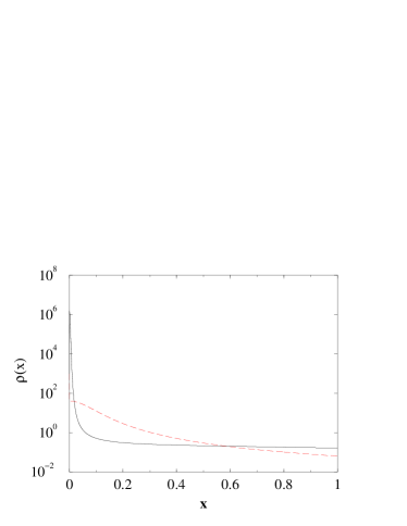
Figure 2: MF density profiles $\rho_{u}({x})$ of a uniform state (dashed line) and $\rho_{c-h}({x})$ of a core-halo state (solid line) for $\epsilon=\epsilon_{coll}$

$$\rho({\bf x})=\rho_{0}F[\rho(.),{\bf x}]$$

$$F[\rho(.),{\bf x}]=\exp\left[\beta\int{\rho({\bf x}^{\prime})\over\sqrt{({\bf x}-{\bf x}^{\prime})^{2}+x_{0}^{2}}}d^{3}{\bf x}^{\prime}\right]$$

$$\beta={3\over 2}\left[\epsilon+{1\over 2}\int\int{\rho({\bf x}_{1})\rho({\bf x}_{2})\over\sqrt{({\bf x}_{1}-{\bf x}_{2})^{2}+x_{0}^{2}}}d^{3}{\bf x}_{1}d^{3}{\bf x}_{2}\right]^{-1}$$ (2)

$$\rho_{0}=\left\{\int F[\rho_{s}(.),{\bf x}]d^{3}{\bf x}\right\}^{-1}$$

The equilibrium density profile $\rho({x})$ obtained from this equation is then used to calculate the entropy and the pressure.

The MF phase diagram of the system is presented in Fig. 1. The collapse and explosion energies are $\epsilon_{coll}\approx-0.339$ and $\epsilon_{expl}\approx 0.267$. Examples of the uniform and the core-halo density profiles for $\epsilon=\epsilon_{coll}$ are shown in Fig. 2.

In the MD simulations we consider a system consisting of $N=125$ – 500 particles in a spherical container of the radius $R=1$. All interparticle forces are calculated directly at each time step $dt$. This is done to avoid any mean-field-like effects inevitably present in any truncated multipole or Fourier potential expansion. The particle velocities and coordinates are updated according to the velocity-Verlet algorithm which is symplectic and reversible.

The system is initialized by randomly distributing particles according to a spherically symmetric density profile; typically the appropriate MF density profile $\rho(x)$ was used. The potential energy ($U$) of the initial configuration is calculated, and the target kinetic energy $E_{k}=E-U$ is determined. The particle velocities are randomly generated from some (usually Maxwell) distribution with the appropriate square average. Finally, the deviation of the total energy from its target value, caused by a stochasticity in velocity assignment, is determined, and the velocities are rescaled to fine-tune the total energy. Due to the isotropicity of the random velocity assignment, we have always obtained the states with sufficiently low total angular momentum which collapsed to single-core states rather than to binaries grv .

To implement the reflective boundary condition, at each time step the normal components $v_{\perp}$ of the velocities of all particles which had escaped from the container were reversed. Values of the normal components were stored to evaluate the pressure on the wall $P$.

$$P(t)=\frac{\sum_{t^{\prime}=t-t^{\prime\prime}/2}^{t^{\prime}=t+t^{\prime\prime}/2}v_{\perp}(t^{\prime})}{2\pi R^{2}t^{\prime\prime}}$$ (3)

During each simulation run we measured such characteristics as the kinetic energy $\epsilon_{kin}=\frac{3}{2\beta}$, the virial variable $\sigma$ (dimension of energy) quantifying deviations from the virial theorem, $\sigma\equiv\epsilon+\epsilon_{kin}-\frac{3PVR}{N^{2}}$ (where $P$ is the pressure on the wall, $V=4\pi R^{3}/3$ is volume of the container, and the factor $N^{2}/R$ rescales the volume-pressure term to the unit of energy introduced in (II)), ratio of the velocity moments, $\frac{19\langle v^{2}\rangle^{2}}{5\langle v^{4}\rangle}$ (which should be 1 for the Maxwell distribution), and the number of particles in the core $N_{c}$ of the prescribed radius $x_{c}$. For the last measurement we count the number of particles $N_{i}$ that are within $x_{c}$ from the $i$th particle and find the particle which has the largest $N_{i}$.

In addition, we measured the histograms of the velocity distribution and radial distribution functions, $W(u)$ and $C(x)$, respectively. The latter was defined as the number of particles in the spherical layer of the radius $x$ around each particle, normalized by the volume of such layer, disregarding the nonuniformity of the system and the boundary effect.

The measurements of the ”scalar” quantities such as energy, kinetic energy, pressure, and velocity distribution moments were taken in time intervals $\tau_{meas}$, which were selected sufficiently long to avoid measuring the unchanged configuration repeatedly and sufficiently short not to miss the important details of the system evolution. We usually pick $\tau_{meas}$ of the order of the uniform density sphere crossing time $\tau_{cross}^{u}=\pi$, which is a half period of the oscillation of a particle released with zero velocity at the container wall. The histogram data, such as the velocity distribution and the radial distribution functions, was incremented at each $\tau_{meas}$ and accumulated over a longer time period $\tau_{hist}$, $\tau_{hist}\sim 10$ – $10^{3}\times\tau_{meas}$.

Our attempts to resolve the high-density part of the radial density profile of the system turned out to be fruitless due to the strong fluctuations in the positions of this part. This fluctuations result in smearing the central peak in both core-halo and low energy uniform states. Considering the center of mass system of reference does not resolve this difficulty, as, despite being dense, the core typically contains only 10 – 20% of the total system mass (see below) and the positions of the core and the center of mass of the system do not usually coincide.

To control the quality of the simulation, we monitored the total energy $\epsilon$ and the total angular momentum $L$. We selected timestep $dt$ small enough to keep the total energy variation within 0.01% of its initial value, usually we used $dt=10^{-5}$, or in rescaled units, $d\tau\sim 10^{-4}$. For such time steps, the relative deviation of the angular momentum was within $10^{-14}$.

All the measurements below are presented in the rescaled dimensionless units as defined in Eq. (II).

III uniform and core-halo equilibrium states: comparison to the MF

To check our simulation procedure and possibly resolve the apparent contradiction between the MF and the particle simulation results pet , we first considered the system in what we expected to be a stable or a metastable states far away from a transition point. Since we were interested in the equilibrium properties, we were initiating the MD systems according the corresponding MF predictions. It meant that the density profiles were seeded according to the MF profiles and the velocities were assigned according to the Maxwell distribution. We observed that the MF density initiation virtually eliminates the transitory period, while the method of velocity assignment was practically unimportant, provided that it gave the correct value for the total kinetic energy. For example, it takes a system initialized with a flat $W({\bf u})=const$ about $\tau\sim\tau_{r}$ to evolve to the Maxwell distribution.

A typical plot of the steady state time dependence of the kinetic energy, virial variable, and the total energy is presented in Fig. 3.

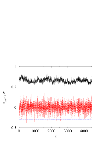
Figure 3: Plots of time dependence of kinetic energy $e_{kin}$ (solid line), virial variable $\sigma$ (dashed line), and total energy $\epsilon$ (dotted line) for a uniform system of $N=250$ particles at $e=-0.3$.

The comparison between the MD measurements and the MF results for the uniform and core-halo states is presented in Tables LABEL:tab_un and LABEL:tab_ch and reveals a perfect agreement between these two sets of data.

Table 1: Equilibrium MD and MF results for a uniform state for $\epsilon=-0.3$, $N=250$, and $0\leq\tau\leq 5000$

	MD	MF
$\epsilon$	$-0.3\pm 5\times 10^{-7}$	-0.3
$\epsilon_{kin}$	$0.66\pm 0.05$	0.644
$\sigma$	$0\pm 0.03$	0.012
$19\langle v^{2}\rangle^{2}/5\langle v^{4}\rangle$	$1.01\pm 0.04$	1

Table 2: Equilibrium MD and MF results for a core-halo state at $\epsilon=-0.339$, $N=250$, and $0\leq\tau\leq 1500$

	MD	MF
$\epsilon$	$-0.3392\pm 2\times 10^{-4}$	-0.339
$\epsilon_{kin}$	$2.9\pm 0.1$	2.94
$\sigma$	$-1.5\pm 0.1$	-1.46
$19\langle v^{2}\rangle^{2}/5\langle v^{4}\rangle$	$0.99\pm 0.03$	1
$N_{core}$	$48\pm 2$	47.6

To obtain the expression for the MF virial variable

$$\sigma_{MF}=\epsilon+\epsilon_{kin}(1-8\pi\rho(1)/3)$$ (4)

we write for the pressure at the container wall $P=2\rho(x=1)\epsilon_{kin}/3$ implying that the system is isothermal. Since the interparticle potential is not pure Coulombic, the virial variable is non-zero. The difference is especially prominent for the core-halo states where more particles ”probe” the short-range part of the potential.

To evaluate the core radius and number of core particles of the core-halo system, we considered an integrated MF density profile, $f(x)=\int_{0}^{x}4\pi y^{2}\rho(y)dy$ (see Fig. 4).

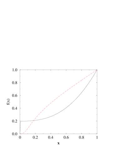
Figure 4: Integrated MF density profiles $f_{u}({x})$ of a uniform state (dashed line) and $f_{c-h}({x})$ of a core-halo state (solid line) for $\epsilon=\epsilon_{coll}$

As it follows from the Figure, the MF core-halo state indeed contains a distinct core with a sharp boundary of the radius $x_{c}\approx 10^{-2}$ relatively insensitive to the energy in the range we considered, $|\epsilon|<0.5$. Using this MF core radius, we located cores in the MD core-halo systems which contained very similar to the MF cores number of particles (see Table LABEL:tab_ch). Using smaller core radius resulted in significant reduction in the number of observed core particles. A reasonably small over-estimation of the core radius did not affect the results of the MD measurements: we observed that even in the sphere twice the core radius the number of particles is only marginally (at most by 8%) larger than in the core.

To check if the system has more than one core, we performed search for the second-largest core of the same radius $x_{c}$. We looked for a largest group of particles which are within $x_{c}$ from a single particle with none of these particles belonging to the first, largest core. We never observed the second-largest core containing more than 2 particles; most of the time it contained only a single one.

In Fig. 5 we present the MD velocity distribution functions $W(u)$ for a core-halo and uniform states; shown $W(u)$ confirm the MF prediction for the Maxwellian form of these distributions.

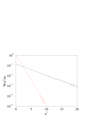
Figure 5: The MD velocity distribution functions $W(u)$ of a core-halo state with $\epsilon=-0.339$ (solid line) and a uniform state with $\epsilon=-0.3$ (dashed line). In both cases $N=250$.

As we mentioned in the previous section, we were unable to resolve the high-density part of the radial density profile due to the core motion. However, an indirect comparison between the radial distribution of particles in the MF and MD was made using the radial distribution function. The MF radial distribution function $C_{MF}(x)$ was computed as

$$C_{MF}(x)=\frac{1}{4\pi x^{2}}\int\rho({\bf x}^{\prime})\rho({\bf x+x}^{\prime})d{\bf x}^{\prime}.$$ (5)

The good agreement between the MF and the MD radial distribution functions is illustrated in Fig. 6. This indicates that the mutual distribution of particles is correctly predicted by the MF theory.

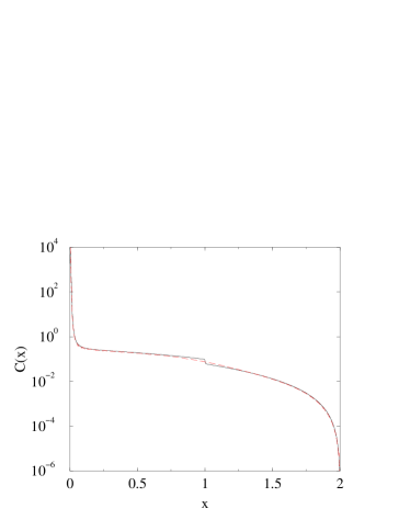
Figure 6: MF (dashed line) and MD (solid line) radial distribution functions $C(x)$ of a core-halo state with $\epsilon=0.25$. The step at $x=1$ in the MF $C(x)$ is caused by the localization of the core exactly at $x=0$ and a sharp boundary of the container.

To summarize, for all the quantities considered, we observed no systematic deviations between the MF theory and the MD data.

IV Collapse

According to the MF theory, if the energy of the uniform state becomes lower than $\epsilon_{coll}\approx-0.339$, the system should undergo a collapse to a core-halo state. To study the collapse, we considered several uniform systems with the energies ranging between $\epsilon=-0.5$ and $\epsilon=-0.3$. The systems were initialized according to the MF density distributions. For systems with $\epsilon<\epsilon_{coll}$ the particles were distributed according to the MF density profile for $\epsilon_{coll}$.

In a perfect agreement with the MF theory, a uniform state with $\epsilon<\epsilon_{coll}$ undergoes a gradual transition to a core-halo state with a typical timescale of $\tau_{coll}\sim 10^{4}$ for $N=125$ – 250 particles. An example of the time dependence of the kinetic energy and the virial variable for a collapsing system is shown in Fig. 7.

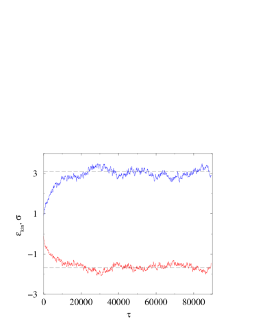
Figure 7: Time dependence of the kinetic energy $\epsilon_{kin}$ (top) and the virial variable $\sigma$ (bottom) of the collapsing uniform state with $\epsilon=-0.5$ and $N=125$. The dashed horizontal lines indicate the equilibrium values of $\epsilon_{kin}$ and $\sigma$ of the corresponding core-halo state. The data is averaged over $\delta\tau=100$ time intervals.

We observe that if the number of particles is increased but the rescaled energy $\epsilon$ is kept fixed, it takes generally longer time for the collapse to be complete. Our results (see Fig. 8) qualitatively confirm that the characteristic time for the full collapse scales as $\tau_{r}$ bt . A quantitative study of the dependence of the collapse dynamics on the number of particles requires much faster simulation code, however.

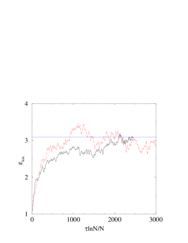
Figure 8: Collapse in systems with $\epsilon=-0.5$ and different numbers of particles, $N=125$ (dashed line) and $N=250$ (solid line), shown in relaxation time units, $\tau\ln N/N$ bt . Horizontal line shows the kinetic energy of the target core-halo state. The data is averaged over $\delta\tau=100$ time intervals.

In the above examples, the energy was set to $\epsilon=-0.5$ which is well below $\epsilon_{coll}\approx-0.339$, and as a consequence the collapse started immediately at $\tau=0$ in all simulation runs. If the system energy is $\epsilon_{coll}$, the noticeable increase in kinetic energy and decrease of the virial variable, characteristic for collapse, start not exactly at $\tau=0$ but with a small delay (Fig. 9) which varies from run to run from almost zero to about $\tau\approx 1500$. This indicates that the MD system is able to overcome the metastability at or near $\epsilon_{coll}$. The observed uncertainty is likely due to the relatively small number of particles.

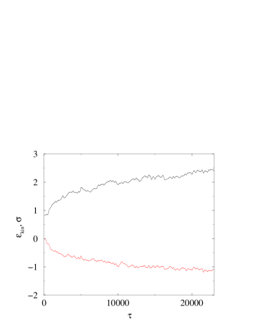
Figure 9: Plots of the kinetic energy $\epsilon_{kin}$ (top) and the virial variable $\sigma$ (bottom) vs time $\tau$ for a system with $\epsilon=\epsilon_{coll}\approx-0.339$ and $N=250$.The data is averaged over $\delta\tau=100$ time intervals.

As we increase the energy above $\epsilon_{coll}$, the stability of the uniform state increases which results in a longer lifetime of such state with respect to collapse. In Fig. 10, an evolution of a system with $\epsilon=-0.3$ is shown. The system stays in the uniform state for about $\delta\tau\approx 5000$ before the collapse starts, after which the evolution proceeds qualitatively similar to the collapses in systems with lower energies.

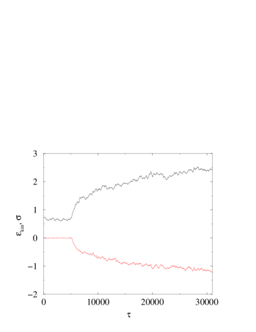
Figure 10: Plots of the kinetic energy $\epsilon_{kin}$ (top) and virial variable $\sigma$ (bottom) vs time $\tau$ for a system with $\epsilon=-0.3$ and $N=250$. The data is averaged over $\delta\tau=100$ time intervals.

To compare the temporal evolution of the kinetic energy, virial variable, and the number of core particles, the relative variables $\epsilon^{\prime}_{kin}(\tau)$, $\sigma^{\prime}_{kin}(\tau)$, and $N^{\prime}_{core}(\tau)$, all defined as $\epsilon^{\prime}_{kin}(t)=[\epsilon_{kin}(t)-\epsilon_{kin}(u)]/[\epsilon_{kin}(c-h)-\epsilon_{kin}(u)]$, are plotted in Fig.11. The values $\epsilon_{kin}(u)$ and $\epsilon_{kin}(c-h)$ correspond to the uniform and core-halo states in equilibrium.

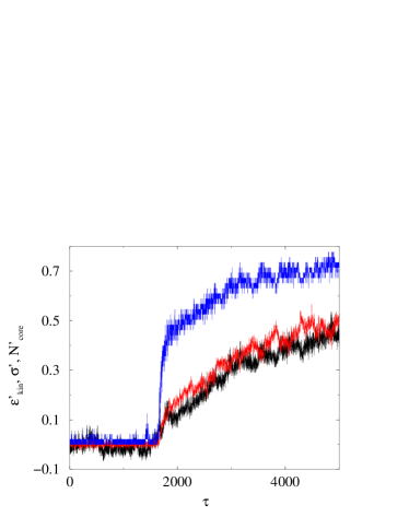
Figure 11: Plots of the relative values of (from top to the bottom) number of core particles $N^{\prime}_{core}(\tau)$, virial variable $\sigma^{\prime}_{kin}(\tau)$, and kinetic energy $\epsilon^{\prime}_{kin}(\tau)$ for the system with $\epsilon=-0.339$ and $N=250$.

Figure 11 indicates that during the initial stages of collapse the core grows faster than the kinetic energy and the virial variable. In addition, one can notice large reversible fluctuations in the number of core particles (the core grows up to 12% of its final value and then disappears) that are not matched by comparable scale fluctuations in the kinetic energy or virial variable. All these observations suggest that the density evolution causing the core formation plays the leading role in the process of collapse while the relaxation of kinetic energy follows. Once the collapse has started, the core grows to about a half of its final size in only $\delta\tau_{core}\sim 10^{3}$ for systems with $N=125$ – 500 particles, while the changes in kinetic energy during this interval of time are small. After this rapid initial stage the system relaxes more slowly, and finally after $\tau_{coll}\sim 10^{5}$ reaches the equilibrium core-halo state. Our observations strongly suggest that the growth of the core takes place through a sequential absorption of single particles rather than through hierarchical merging of smaller cores: We never detected other cores containing more than two particles. Although the kinetic energy relaxation trails behind the the core formation, the velocity distribution function remains Maxwellian throughout the whole evolution with the temperature corresponding to the corresponding value of the kinetic energy. This is caused by the fast velocity relaxation ($\tau_{vel}\leq 1$) as discussed in the previous section.

V Explosion

It is natural to assume that if a system exhibits a collapse, it should also exhibit an explosion which is the reverse to the collapse transition. According to the MF theory, such explosion should take place when the core-halo state becomes unstable, i.e., when $\epsilon\geq\epsilon_{expl}\approx 0.267$. To check this prediction, we initialized the MD system according to the MF equilibrium core-halo state and followed its evolution. As in the study of the collapse, for initial states with $\epsilon>\epsilon_{expl}$ we used the MF density profiles of the highest energy locally stable state, i.e. of the state with $\epsilon=\epsilon_{expl}$.

We observe that a system with sufficiently high energy, such as $\epsilon=0.5$ in Fig. 12 or $\epsilon=0.4$ in Fig. 13, indeed undergoes an explosion which brings it to the uniform equilibrium state. During such an explosion, the state variables such as kinetic energy and virial variable continuously change from their equilibrium core-halo state values to the uniform state ones, and the core gradually sheds particles until only one particle is left.

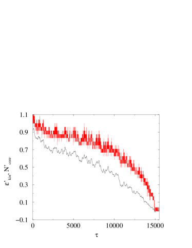
Figure 12: Plots of the kinetic energy $\epsilon^{\prime}_{kin}(\tau)$ (top) and relative number of core particles $N^{\prime}_{core}(\tau)$ (bottom) (defined as in Fig. 11) vs time $\tau$ for a system with $\epsilon=0.5$ and $N=250$. The kinetic energy is averaged over $\delta\tau=100$ time intervals.

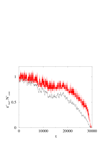
Figure 13: Same as in Fig. 13 but for $\epsilon=0.4$.

The main features of an explosion (Figs. 12 and 13) resemble those of a time-reversed collapse. The kinetic energy evolves relatively uniformly, while the number of core particles changes only slightly during the first stages of evolution and rapidly decreases at the final stages. In the example presented in Fig. 12, the explosion is complete after the time $t_{expl}\approx 15000$, which is noticeably less than the time for a collapse $t_{coll}\approx 10^{5}$ (see Fig. 8) for a system having the same number of particles ($N=250$). However, the latter is rather vaguely defined due to larger fluctuations in a core-halo than in a uniform state.

Similarly to a collapse, the system remains thermalized in the velocity space during an explosion. The velocity distribution remains Maxwellian throughout the evolution with the temperature corresponding to the current value of kinetic energy. As an illustration, Fig. 14 shows the ratio of the moments of velocity distribution, $19\langle v^{2}\rangle^{2}/5\langle v^{4}\rangle$, which should be 1 for a Gaussian distribution.

Figure 14: Plot of he ratio of the moments of velocity distribution, $19\langle v^{2}\rangle^{2}/5\langle v^{4}\rangle$, vs.time $\tau$ for a system with $\epsilon=0.5$ and $N=250$.

However, as it is evident from a comparison between the Figs. 12 and 13, as $\epsilon$ gets closer to $\epsilon_{expl}$ the explosion takes longer to initiate. We have observed, that even for $\epsilon=0.3$, which is noticeably larger than $\epsilon_{expl}\approx 0.267$, the explosion does not happen during the first $\tau=30000$ of evolution. This suggests that either the MF value for $\epsilon_{expl}$ is incorrect, or during the incitation of the system we somehow prepare the system not exactly in the equilibrium (metastable) core-halo state. If the latter is the case, a deviation from the equilibrium most probably takes place in the core, as because of its compactness, its equilibration with the rest of the system may take a rather long time. Using the current MD setup, we were unable to determine a reason for this apparent discrepancy.

VI CONCLUSION

In the previous sections we have presented the following molecular dynamics results for the self-attracting systems with soft Coulomb potential:

• A collapse from a uniform to a core-halo state was observed. The timescale for the collapse in systems consisting of 125 – 500 particles is of order of $10^{5}$ crossing times and is by the same factor longer than the timescale of the velocity relaxation. The collapse starts with a fast growth of a core via absorption of single particles and continues with more gradual relaxation towards an equilibrium core-halo state. Metastable states exhibit a finite lifetime before collapsing.

• A reverse to collapse, i.e., an explosion transition from a core-halo to a

  uniform state was observed. The explosion time is considerably shorter than the collapse time, being of the order of $10^{4}$ crossing times (125 – 500 particles). An explosion resembles a time-reversed collapse; the core decrease, which happens by shedding individual particles, is trailing the kinetic energy evolution till the last stages, when the core rapidly disappears.

• Such molecular dynamics characteristics of the equilibrium or the metastable uniform and core-halo states as kinetic energy, wall pressure, number of core particles, particle-particle radial distribution function and velocity distribution function, are found to be equal within the statistical uncertainty of the molecular dynamics measurements to the corresponding mean field predictions.

The long collapse time observed in our simulations appears to be an explanation for the apparent discrepancy between the phase diagram presented in pet and the mean field phase diagram (see, for example, chi ). The relaxation time allowed in pet before the measurements of what was considered to be a steady state, $t_{rel}=3N/|EN|^{3/2}$, which is apparently equivalent to $\tau_{rel}<1$, is by far insufficient for a system to collapse. Therefore, the discontinuities in caloric curves $\beta$ vs $\epsilon$, typical for collapse and explosion gravitational transitions, were not observed in pet .

Although we considered systems only with the soft Coulomb potential, we speculate that a likewise similarity between the mean field and molecular dynamics equilibrium properties of the core-halo state exists for all ”soft” long-range (like a Fourier-truncated Coulomb) potentials. This is so because all soft potentials are effectively longer-ranged than the bare Coulomb one. However, the core-halo state in the system with a ”harder” short-range cutoff may have completely different properties from the one considered above, and its mean field theory may be inadequate. As for the uniform states, their properties are virtually independent on the nature of the cutoff (see, for example, chi ) and their mean-field description is universally correct.

The main goal in the paper was to check the existence of collapses and explosions and the validity of the mean field data for the self-gravitating systems with short-range cutoff. For this goal one or few molecular dynamics runs for each considered system were sufficient. However, to be able to study the dynamical features of collapses and explosion in more detail and to compare the simulations results to various theoretical models, one needs to study the relaxation averaged over many initial configuration. For example, an interesting question is whether a collapse (or an explosion) indeed consists of two stages; the first fast stage of collisionless ”violent relaxation” with particle number-independent rate, and the slower second stage of soft collisional relaxation with characteristic time $\tau_{r}$ (see, for example, bt and references therein). Another important question is to resolve the apparent contradiction between the mean field prediction for $\epsilon_{expl}$ and the molecular dynamics observations, outlined at the end of the previous section. Such studies require a more efficient computation code. The main improvement possibly coming from a better force calculator that may include various mean-field-like potential expansions, which are qualitatively justified by this study. We leave this for the future research.

VII acknowledgments

The authors are thankful to P.-H. Chavanis and E. G. D. Cohen for helpful and inspiring discussions and gratefully acknowledge the support of Chilean FONDECYT under grants 1020052 and 7020052. M. K. would like to thank the Department of Physics at Universidad de Santiago for warm hospitality.

References

- (1) T. Padmanabhan, Phys. Rep. 188, 285 (1990).
- (2) B. Stahl, M. K.-H. Kiessling, and K. Schindler, Planet. Space Sci. 43, 271 (1995).
- (3) P.-H. Chavanis and J. Sommeria, Mon. Not. R. Astr. Soc. 296, 569 (1998).
- (4) V. P. Youngkins and B. N. Miller, Phys. Rev. E. 62, 4583 (2000).
- (5) I. Ispolatov and E. G. D. Cohen, Phys. Rev. E. 64, 056103 (2001), Phys. Rev. Lett. 87, 210601 (2001).
- (6) H. J. de Vega and N. Sánchez, Nucl. Phys. B 625, 409 (2002)
- (7) P.H. Chavanis, Phys. Rev. E. 65, 056123 (2002)
- (8) P.H. Chavanis, C. Rosier, and C. Sire, Phys. Rev. E. 66, 036105 (2002).
- (9) S. Chandrasekhar, An Introduction to the Study of Stellar Structure (Dover Publications, 1958), Ch. 11.
- (10) P.H. Chavanis, I. Ispolatov, Phys. Rev. E. 64, 056103 (2001)
- (11) J. Binney and S. Tremaine Galactic Dynamics (Princeton Series in Astrophysics, 1987).
- (12) J. Katz and I. Okamoto, Mon. Not. R. Astr. Soc. 317, 163 (2000).
- (13) M. Cerruti-Sola, P. Cipriani, and M. Pettini, Mon. Not. R. Astr. Soc. 328, 339 (2001).
- (14) P. Hut, M. M. Shara, S. J. Aarseth, R. S. Klessen, J. C. Lombardi Jr., J. Makino, S. McMillan, O. R. Pols, P. J. Teuben, R. F. Webbink, to appear in New Astronomy, astro-ph/0207318.
- (15) C. Lancellotti and M. Kiessling, Astrophys. J. 549, L93 (2001).
- (16) E. V. Votyakov, H. I. Hidmi, A. De Martino, D. H. E. Gross, Phys. Rev. Lett., 89, 031101 (2002).