Inferring Pattern and Disorder in
Close-Packed Structures from X-ray Diffraction Studies, Part I:
$\epsilon$-Machine Spectral Reconstruction Theory

Abstract

In a recent publication [D. P. Varn, G. S. Canright, and J. P. Crutchfield, Phys. Rev. B 66:17, 156 (2002)] we introduced a new technique for discovering and describing planar disorder in close-packed structures (CPSs) directly from their diffraction spectra. Here we provide the theoretical development behind those results, adapting computational mechanics to describe one-dimensional structure in materials. By way of contrast, we give a detailed analysis of the current alternative approach, the fault model (FM), and offer several criticisms. We then demonstrate that the computational mechanics description of the stacking sequence—in the form of an $\epsilon$-machine—provides the minimal and unique description of the crystal, whether ordered, disordered, or some combination. We find that we can detect and describe any amount of disorder, as well as materials that are mixtures of various kinds of crystalline structure. For purposes of comparison, we show that in some special limits it is possible to reduce the $\epsilon$-machine to the FM’s description of faulting structures. The comparison demonstrates that an $\epsilon$-machine gives more physical insight into material structures and also more accurate predictions of those structures. From the $\epsilon$-machine it is possible to calculate measures of memory, structural complexity, and configurational entropy. We demonstrate our technique on four prototype systems and find that it provides stacking descriptions that are superior to any so far used in the literature. Underlying this approach is a novel method for $\epsilon$-machine reconstruction that uses correlation functions estimated from diffraction spectra, rather than sequences of microscopic configurations, as is typically used in other domains. The result is that the methods developed here can be adapted to a wide range of experimental systems in which spectroscopic data is available.

I Introduction

Fundamental to understanding the physical properties of a solid is a thorough description of its composition and the arrangement of its constituent parts. While chemical analysis provides information about composition, many complementary methods—such as x-ray diffraction, electron diffraction, high-resolution electron microscopy, optical microscopy, and x-ray diffraction tomography—are essential to discovering the large-scale structure of crystalline materials. For example, the placement of Bragg peaks in x-ray diffraction spectra has proved to be a particularly powerful source of structural information in ordered solids for nearly a century. von Laue (1918) For solids that deviate from a strict periodic ordering of their constituent atoms, however, the diffraction spectrum typically shows a weakening and broadening the Bragg peaks as well as the appearance of diffuse scattering. As the disorder becomes more pronounced, the Bragg peaks disappear altogether and leave a completely diffuse spectrum. The problem of inferring crystal structure for such disordered materials from x-ray diffraction has been addressed by many researchers.Frey (1995); Jagodzinski (1987); Proffen and Welberry (1998); Welberry (1985); Schulz (1982); Guinier (1963) In the most general case, however, the problem remains unsolved. Indeed, it is known that without the assumption of strict crystallinity, the problem has no unique solution. Woolfson (1997)

Many kinds of disorder are present in solids, Hirth and Lothe (1982); Ashcroft and Mermin (1976); Kittel (1996) such as Schottky defects, substitution impurities, screw and edge dislocations, and planar slips. Of these, only planar slips will be considered here. Planar defects occur in crystal structure when one crystal plane is displaced from another by a non-Bravais lattice vector. These slips can occur during crystal growth or can result from some stress to the crystal, be it mechanical, thermal, or even through irradiation. Sebastian and Krishna (1994) When an otherwise perfect crystal has some planar disorder, the portion of the structure that cannot be thought of as part of the crystal is called a fault. If there is a transition between two crystal structures, the interface between the two is also known as a fault, even if each layer can be thought of as belonging to one of the crystal structures. Many different kinds of faults have been postulated, including growth faults, deformation faults, and layer-displacement faults. Sebastian and Krishna (1994); Frank (1951a); Frey and Boysen (1981)

Planar defects are surprisingly common in crystals, being especially prevalent in a broad class of materials know as polytypes.Verma and Krisha (1966); Sebastian and Krishna (1994); Trigunayat (1991); Pandey and Krishna (1982); Frevel et al. (1992) First discovered in SiC by Baumhauer Baumhauer (1912) in 1912, polytypism has since been found in dozens of materials. Polytypism is the phenomenon of solids built up from identical not (a) layers, called modular layers (MLs), Varn and Canright (2001) that differ only in the manner of the stacking. Typically, one finds that the intra-ML interactions are relatively strong as compared to the inter-ML interactions, so that disorder within a ML is rare. Energetic considerations usually restrict the allowed orientations of MLs to a discrete set, with only a small energy difference between two different stackings. Thus, the description of a polytype, ordered or disordered, formally reduces to a one-dimensional list—called the stacking sequence—that lists successive orientations encountered as one moves along the stacking direction.

The small energy difference between different stackings arises because the coordination of the nearest neighbor, next-nearest neighbor, and sometimes even higher neighbors is often the same regardless of the stacking arrangement. It is therefore possible to have many distinct stackings—some periodic and some not. For several of the most polytypic materials—e.g., SiC, ZnS, and CdI₂—there are about $150$, $185$, and $200$ known crystalline structures, respectively. Remarkably, some have unit cells extending over 100 MLs. Sebastian and Krishna (1994) The stacking period of many such polytypes is far in excess of the calculated inter-ML interactions, which are estimated to be, for example, $\sim 1$ ML in ZnS Engel and Needs (1990) and $\sim 3$ ML in SiC. Cheng et al. (1987); Shaw and Heine (1990) Nearly a dozen theories have been proposed, Sebastian and Krishna (1994); Trigunayat (1991); Frank (1951b); Pandey and Krishna (1982); Jagodzinski (1954); Yeomans (1988); Pandey (1989) yet a satisfactory and systematic explanation is still lacking for the diversity and kinds of observed structure.

Much of the interest in polytypism has centered around the issue of long-range order and the existence of so many apparently stable structures. Reconciling the calculated range of interaction between MLs with the length scale over which organization appears has been the chief mystery of polytypism. Also of interest is the characterization of the solid-state transformations common in many of these materials. While the length scale on which spatial organization appears in these materials is easily found for crystal structures, the similar question for disordered structures has not so far been addressed. What is needed is a model is that gives a statistical description of the observed stacking sequences from which characteristic length parameters are calculable. Finally, from a unified description of both crystalline and noncrystalline structures, a more comprehensive picture of polytypism should emerge and hopefully render polytypism more amenable to theoretical discussion and analysis.

A significant source of information about the structure of solids is derived from diffraction spectra. While it can be challenging to identify crystal structures with units cells over 100s of MLs, in fact most periodic structures have been identified. Sebastian and Krishna (1994) In many polytypes, disordered sequences are also common, and a single crystal can contain regions of both ordered and disordered stackings. A main goal of this present work is to develop a technique for discovering and describing planar disorder in close-packed structures (CPSs) from diffraction spectra. A further task is to detail the connection between our model of disordered structures and physically relevant parameters derivable from it. We will then be in a position to treat similar questions about the possibility of long-range order in disordered structures.

I.1 Indirect Methods

The problem of quantifying the effects of planar disorder on diffraction spectra has a long history. (For a more complete discussion, see Sebastian and Krishna. Sebastian and Krishna (1994)) Perhaps the first quantitative analysis was given by Landau Landau (1937) and Lifschitz Lifschitz (1937) assuming no correlation between MLs. Wilson Wilson (1942) provided an analysis of planar imperfections in hexagonal Co by considering the effect of the disorder on the Bragg peaks. This approach is necessarily limited to the case of small amounts of faulting. Hendricks and Teller Hendricks and Teller (1942) treated the problem rather generally, allowing for different form factors for the different kinds of MLs, variable spacing between MLs, and correlations between neighboring MLs. Since their method relies on extensive matrix calculations, it was found cumbersome and difficult to apply by early researchers.

Jagodzinski developed a theory of diffraction for planar disorder by considering nearest-neighbor correlations for general layered structures Jagodzinski (1949a) and for next-nearest neighbor correlations of CPSs. Jagodzinski (1949b) By noting the direction, length, and intensity of non-Laue streaks in x-ray diffraction spectra of Cu-Si alloys, Barrett Barrett (1950) was able to estimate the kind and approximate amount of stacking disorder present. Patterson Patterson (1952) considered the effect of deformation faults on face-centered cubic crystals (fcc or 3C not (b)) and demonstrated how one can calculate the fraction of faulted layers from the widths and displacements of the Bragg peaks. Gevers Gevers (1954a) demonstrated how to calculate the effects of growth faults with an $n$-layer influence on the diffraction spectra of close-packed crystals. He also demonstrated how to treat both growth and deformation faults randomly inserted into hexagonal (hcp or 2H) and cubic crystals, as well as deformation faults randomly distributed into 4H and 6H crystals. Gevers (1954b) Johnson Johnson (1963) examined the effects on the diffraction pattern of random extrinsic faulting (insertion of a ML) in the 3C structure and compared this to the effects of intrinsic faulting (deletion of a ML) on the Bragg peaks in the limit of small fault probabilities. Prasad and Lele Prasad and Lele (1970) considered the effects of faulting on the diffraction spectra of 4H crystals containing up to nine kinds of randomly distributed faults. Pandey and Krishna Pandey and Krishna (1976) treated the similar case of the 6H close-packed structure containing a random distribution of $14$ distinct intrinsic faults. Pandey and Krishna Pandey and Krishna (1977) also derived an expression for the intensity of diffracted radiation from a 2H crystal containing any amount of randomly placed deformation and growth faults. By measuring the broadening of the diffraction maxima of a SiC crystal they were able to determine the amount of each kind of faulting. Michalski Michalski (1988) developed a general theory for the random distribution of single stacking faults for an arbitrary periodic structure and Michalski, et al. Michalski et al. (1988) applied it to several hexagonal and rhombohedral structures.

In an effort to understand experimental data concerning solid-state transformations from the 2H to the 6H structure in annealed SiC crystals, Pandey et al. Pandey et al. (1980a, b, c) developed the concept of nonrandom faulting. They suggested that the presence of a fault in a structure affects the probability of finding another fault in close proximity. They considered two possible faulting mechanisms—deformation faulting and layer-displacement faults—and were able to understand the stacking in SiC within this model. Similar work was done on the 2H-to-3C transformation in ZnS crystals. Sebastian (1988); Sebastian and Krishna (1984, 1987a, 1987b); Sebastian et al. (1982); Sebastian and Krishna (1994); Frey et al. (1986); Pandey et al. (1980a, b, c); Pandey and Lele (1986a, b); Jagodinski (1972)

All of the above methods center on finding analytical expressions for the diffracted intensity as a function of fault probabilities. In order to make a quantitative estimate of the faulting, typically the placement, broadening, shape, and symmetry of the Bragg peaks are compared with that expected for a crystal containing a particular kind of fault. Then the full width at half-maximum (FWHM) of one or several of the Bragg peaks are used to determine the fraction of faulting.

Thus, all of these approaches are limited to small amounts of disorder that preserve the integrity of the Bragg peaks. (An exception to this is Jagodzinski’s Jagodzinski (1949b) disorder model. This approach has several features in common with our own and can in fact be thought of as a constrained case of our approach. We do not discuss his work further here, but treat it and its relation to ours elsewhere. Varn et al. ) Should the disorder become sufficiently large, the Bragg peaks become too broad and do not stand out sufficiently from the diffuse, background scattering. We call these kinds of approaches indirect, because one begins with a set of postulated faults and then sorts though them, searching for one or several that best fit the data.

I.2 Direct Methods

Perhaps the first efforts at a direct method for determining the structure of disordered close-packed crystals were given by Dornberger-Schiff Dornberger-Schiff (1972) and Farkas-Jahnke. Farkas-Jahnke (1973a, b) Dornberger-Schiff gave an algorithm for relating Patterson values (i.e., fractions of faulted layers from Bragg peaks) to sequence probabilities but, to our knowledge, did not follow up with a method for finding the Patterson values from spectra showing diffuse scattering. Farkas-Jahnke used Patterson-like functions to estimate the frequency of occurrence of layer sequences up to length five. He was not able to obtain a complete set of equations and this forced the use of inequalities derived from symmetry arguments that do not generally hold in disordered crystals. Unlike the previously considered techniques, these methods are direct since they make no assumption about underlying crystal structure or the faults it may contain. To our knowledge, since their introduction three decades ago, neither of these methods have been used to discover stacking structure in real materials. Hence we do not treat them further here.

I.3 The Fault Model

We refer to the indirect approaches—analyzing a crystal structure assuming it contains a distribution of stacking errors or faults—as the fault model (FM). To date, it has been the dominant way in which planar disorder in crystals has been viewed. However, we find a number of difficulties with the FM, many of which have been recognized by previous researchers. Gosk (2000); Proffen and Welberry (1998); Palosz and Przedmojski (1976); Farkas-Jahnke (1973a); Treacy et al. (1991); Michalski (1988) Our objections to the FM and the way it has been used to discover structural information are severalfold.

(i) The FM assumes a parent crystal. For the fault model to make sense, it is necessary to assume some crystal structure in which to introduce faulting. This may be satisfactory for weakly faulted crystals, but for those with significant disorder or those undergoing a solid-state phase transition to another crystal structure, Frey et al. (1986); Jagodinski (1972); Kabra and Pandey (1988a); Krishna and Marshall (1971a, b); Pandey and Lele (1986a, b); Pandey et al. (1980a, b, c); Sebastian et al. (1982); Sebastian and Krishna (1987a, b, c); Sebastian et al. (1987); Shrestha and Pandey (1996a, b); Shrestha et al. (1996); Shrestha and Pandey (1997) this picture is untenable.

(ii) Each parent crystal must be treated separately. Since the FM introduces stacking “mistakes” into a parent crystal, each kind of parent crystal must be treated individually. There has been significant work on only two CPSs; namely, the 2H and 3C. In polytypism hundreds of other crystalline structures are known to exist. In the FM, each must be analyzed separately by postulating appropriate crystal-specific kinds of defects. Given this degree of complication, it is desirable to find a theoretical framework that unites the description of the various kinds of fault and parent structure into a single, coherent picture.

(iii) In practice, the FM treats only the Bragg peaks quantitatively, effectively ignoring the diffuse scattering. Most researchers use formulæ that give the FWHM of Bragg peaks in terms of the fraction of certain postulated defects to find the amount of faulting. Some do acknowledge that diffuse scattering is important, but to our knowledge none use the diffuse scattering to quantitatively measure crystal structure. not (c)

(iv) The FM is unable to capture the variety of naturally occurring stacking sequences. By assuming a small set of possible ways that a parent structure can deviate from crystallinity, the FM necessarily assumes that there are stacking sequences that do not occur. It is desirable to have an approach that considers as many candidate structures as possible with as few a priori restrictions as possible.

(v) The FM’s description of the disorder is not unique. It is possible to give two different faulting schemes that describe the same weakly faulted material. Varn et al. (2002a) This is readily seen by noting that the layer-displacement fault in a 2H crystal can be viewed as two adjacent, but oppositely oriented deformation faults.

I.4 Computational Mechanics

Our method of discovery and quantification of planar structure and disorder in crystals overcomes all of these difficulties for the special but important case of CPSs. We do not assume an underlying crystalline structure. Indeed, we make no assumptions at all about either the crystal or fault structure that may be present. Instead, we find the frequency of occurrence of all possible stacking sequences up to a given length and use this to construct a model that captures the statistics of the stacking sequence. In this sense, we directly determine the stacking structure. Our scheme for describing planar disorder unites both fault and crystal structure into a single framework. There is no need to treat each crystal structure or faulting scheme separately. Our method treats any amount and kind of planar disorder present. Finally, we quantitatively use all of the information contained in the diffraction spectra, both in Bragg peaks and in diffuse scattering, to build a unique model of the stacking structure. This model does not find the particular stacking sequence of the specimen that generated the diffraction pattern—this is not possible from diffraction spectra alone—but rather finds the statistical regularities across an ensemble of stacking sequences that could have given rise to the observed spectra. This is the best that can be done, in principle.

The history of discovering planar disorder in crystals is one of consistent, incremental progress over nearly seventy years. There are two factors, however, that have hindered progress in this area. The first is calculational. Much of the early work centered on finding analytical expressions for the diffracted intensity of a given crystalline structure permeated with a particular fault type. With the advent of modern numerical and symbolic calculational methods and the concomitant ability to estimate diffraction patterns from any arbitrarily layered structure, Treacy et al. (1991) much of this early work has been superseded. The second hindrance to progress has been a lack of fundamental understanding of structure and disorder in one-dimensional sequences generated by nonlinear dynamical systems. Recently, however, a unifying framework has been introduced in theory of computational mechanics. Crutchfield and Young (1989); Crutchfield and Feldman (1997, 2003); Feldman and Crutchfield (1998); Shalizi and Crutchfield (2001); Feldman (1998)

Computational mechanics is an approach to discovering, describing, and quantifying patterns. It provides for the construction of the minimal and unique model for a process that is optimally predictive; this model is called an $\epsilon$-machine. A process’s $\epsilon$-machine is minimal in the sense of requiring the fewest model components to represent the process’s structures and disorder; it is optimal in the sense that no alternative representation is more accurate; and it is unique in the sense that any alternative which is both minimal and optimally predictive is isomorphic to it. An $\epsilon$-machine’s algebraic structure captures a process’s symmetries and approximate symmetries. From an $\epsilon$-machine measures of a process’s memory, entropy production, and structural complexity can be found. We demonstrate in the sequel Varn et al. (2002b) that knowledge of the $\epsilon$-machine and the energy coupling between MLs allows one to calculate the average stacking energy for a disordered polytype. Before being adapted to the present application to polytypes, computational mechanics had been used to analyze structural complexity in a wide range of nonlinear processes, such as cellular automata, Hansen (1993) the logistic map, Crutchfield and Young (1989, 1990) and the one-dimensional Ising model, Feldman (1998); Crutchfield and Feldman (1997) as well to experimental physical systems, such as the dripping faucet, Gonçalves et al. (1998) atmospheric turbulence, Palmer et al. (2000) and geomagnetic data. Clarke et al. (2001)

Our development here is organized as follows: in §II we give a detailed account of our procedure for discovering and quantifying disorder in CPSs; in §III we compare our approach to the FM; in §IV we treat four prototype polytypes to demonstrate our technique; in §V we discuss several characteristic lengths that can be estimated from our model and we address how they relate to the range of interactions between MLs; and in §VI we give our conclusions.

II $\epsilon$-Machine Spectral Reconstruction

Previous techniques of $\epsilon$-machine reconstruction have used a sequence of data produced by the process. Crutchfield and Young (1989); Crutchfield (1994); Shalizi et al. (2002) Here, the experimental signal comes in the form of a power spectrum, and we need to develop a technique to infer the $\epsilon$-machine from this type of data. We call this new class of inference algorithms $\epsilon$-machine spectral reconstruction—abbreviated $\epsilon$MSR and pronounced “emissary”. We emphasize that our goal remains unchanged—to find the process’s underlying description. It is only the inference procedure that is changed. In this section we give a detailed account of $\epsilon$MSR as applied to the problem of discovering pattern and disorder in CPSs.

We divide $\epsilon$MSR into five steps. First, we extract correlation information from a diffraction spectrum. Second, we use this to estimate stacking-sequence probabilities of a given length. Third, we reconstruct an $\epsilon$-machine from this distribution. Fourth, we generate a diffraction spectrum from the $\epsilon$-machine. And, finally, we compare this $\epsilon$-machine spectrum to the original. If there is insufficient agreement, we repeat the second through fourth steps, estimating stacking-sequence probabilities at a longer length, building a new $\epsilon$-machine, and again comparing with the original spectrum. In the final two subsections, we give relations that can be used to determine the quality of experimental data and briefly review several information- and computation-theoretic quantities of physical import that can be directly estimated from the reconstructed $\epsilon$-machine.

II.1 Correlation Factors from Diffraction Spectra

We start with the conventional assumptions concerning polytypism in CPSs. Namely, we assume that

• the MLs themselves are undefected and free of any distortions;

• the spacing between MLs does not depend on the local stacking arrangement;

• each ML has the same scattering power; and

• the faults extend completely across the crystal.

We make the additional assumption that the probability of finding a given stacking sequence in the crystal remains constant through the crystal. (In statistics parlance, we assume that the process is stationary.)

Let $N$ be the number of hexagonal, close-packed MLs, with each ML occupying one of three orientations, denoted $A$, $B$, or $C$. Ashcroft and Mermin (1976); Kittel (1996); Sebastian and Krishna (1994); Varn and Canright (2001) We introduce three statistical quantities, $Q_{c}(n)$, $Q_{a}(n)$, and $Q_{s}(n)$:Yi and Canright (1996) the two-layer correlation functions (CFs), where $c$, $a$, and $s$ stand for cyclic, anti-cyclic, and same, respectively. $Q_{c}(n)$ is defined as the probability that any two MLs at a separation of $n$ are cyclically related. By cyclic, we mean that if the $i^{\mathrm{th}}$ ML is in orientation $A$ ($B,C$), say, then the $(i+n)^{\mathrm{th}}$ ML is in orientation $B$ ($C,A$). $Q_{a}(n)$ and $Q_{s}(n)$ are defined in a similar fashion. Since these are probabilities, $0\leq Q_{\alpha}(n)\leq 1$, where $\alpha\in\{c,a,s\}$. Additionally, at each $n$ it is clear that $\sum_{\alpha}Q_{\alpha}(n)=1$.

With these assumptions and definitions in place, the total diffracted intensity along the $10.l$ row not (d) can be written as Guinier (1963); Berliner and Werner (1986); Yi and Canright (1996)

$$I(l) = \psi^{2}\biggl{(}\frac{\sin^{2}(\pi Nl)}{\sin^{2}(\pi l)}-2\sqrt{3}\sum_{n=1}^{N}\Bigl{\{}(N-n)\times$$ (1)

$$\mbox{}\bigl{[}Q_{c}(n)\cos(2\pi nl+\frac{\pi}{6})$$

$$\mbox{}+Q_{a}(n)\cos(2\pi nl-\frac{\pi}{6})\bigr{]}\Bigr{\}}\biggr{)},$$

where $l$ is a continuous variable that indexes the magnitude of the perpendicular component of the diffracted wave, $k=2\pi l/c$, and $c$ is the spacing between adjacent MLs. $\psi^{2}$ is a function of $l$ that accounts for atomic scattering factors, the structure factor, dispersion factors, or any other effects for which the experimentally obtained diffraction spectra may need to be corrected. Hahn et al. (1992); Woolfson (1997); Milburn (1973)

It is convenient to work with the intensity per ML, instead of the total intensity, so we define the corrected diffracted intensity per ML, $\mathsf{I}(l)$, as

$$\mathsf{I}(l)=\frac{I(l)}{\psi^{2}N}~{}.$$ (2)

We will always use $\mathsf{I}(l)$ unless otherwise noted and simply call this the diffracted intensity. Observe that the diffracted intensity $\mathsf{I}(l)$ integrated over any unit $l$-interval is unity regardless of the particular values of the CFs. Varn (2001) We may then use this fact to normalize experimental data.

The form of Eqs. (1) and (2) suggests that the CFs can be found from the diffraction pattern by Fourier analysis. Let us define $\mathsf{X}(n)$ and $\mathsf{Y}(n)$ as

$$\mathsf{X}(n)=\oint\mathsf{I}(l)\cos(2\pi nl)\,dl$$ (3)

and

$$\mathsf{Y}(n)=\oint\mathsf{I}(l)\sin(2\pi nl)\,dl~{},$$ (4)

where the small circle in the integral sign indicates that the integral is to be taken over a unit interval in $l$. It is possible to show Varn (2001) that in the limit $N\rightarrow\infty$

$$Q_{c}(n)=\frac{1}{3}-\frac{1}{3}\Bigl{[}\mathsf{X}(n)-\sqrt{3}\mathsf{Y}(n)\Bigr{]}$$ (5)

and

$$Q_{a}(n)=\frac{1}{3}-\frac{1}{3}\Bigl{[}\mathsf{X}(n)+\sqrt{3}\mathsf{Y}(n)\Bigr{]}~{}.$$ (6)

Thus, the CFs can be found by Fourier analysis of the diffraction spectrum.

II.2 Estimating the Stacking-Sequence Distribution

In the second part of our approach, we estimate the distribution of stacking sequences from the two-layer CFs. First, though, we must consider what kind of information the CFs contain about stacking sequences. Therefore let us define the stacking process as the effective stochastic process induced by scanning the stacking sequence along the stacking direction. It is convenient to represent the stacking sequence in terms of the Hägg notation, Sebastian and Krishna (1994) where one replaces the set of allowed orientations $\{A,B,C\}$ of a ML with a binary alphabet $\mathcal{A}=\{0,1\}$. On moving from the $i^{\mathrm{th}}$ to the $(i+1)^{\mathrm{th}}$ ML, we label each inter-ML transition or spin Varn and Canright (2001) as “1” if the two MLs are cyclically related ($A\rightarrow B\rightarrow C\rightarrow A$) and “0” if the two MLs are anti-cyclically related ($A\rightarrow C\rightarrow B\rightarrow A$). Thus, the stacking constraint that no two adjacent MLs may have the same orientation ($A$, $B$, or $C$) is built into the notation. There is a one-to-one mapping between the stacking orientation sequence and the spin sequence, up to an overall rotation of the crystal; and we use them interchangeably.

We estimate the probability distribution ${\rm P}(\omega)$ of finding sequences $\omega$ averaged over the sample by considering a series of constraints on the sequence probabilities. Some of these constraints are simple consequences of the mathematics; some come from the CFs themselves. From conservation of probability, we have

$${\rm P}(u)={\rm P}(0u)+{\rm P}(1u)={\rm P}(u0)+{\rm P}(u1)~{},$$ (7)

for all $u\in\mathcal{A}^{r}$, where $\mathcal{A}^{{r}}$ is the set of all sequences of length ${r}$ in the Hägg notation. Additionally, we require that the sum of all probabilities of sequences of length ${r}+1$ be normalized, i.e.,

$$\sum_{\omega\in\mathcal{A}^{{r}+1}}{\rm P}(\omega)=1~{}.$$ (8)

Equations (7) and (8) together provide $2^{{r}}$ constraints among the $2^{{r}+1}$ possible stacking sequences of length ${r}+1$.

The remaining $2^{r}$ constraints come from relating CFs to sequence probabilities via the relations

$$Q_{\alpha}(n)=\sum_{\omega\in\mathcal{A}_{\alpha}^{n}}{\rm P}(\omega)~{},$$ (9)

where $\mathcal{A}_{\alpha}^{n}$ is the subset of length-$n$ sequences that generate a cyclic ($\alpha=c$) or an anti-cyclic ($\alpha=a$) rotation between MLs at separation $n$. A sequence generates a cyclic (anti-cyclic) rotation between MLs at separation $n$ if $2m-n=1\pmod{3}$, where $m$ is the number of $1$s ($0$s) in the sequence. We take as many of the relations in Eq. (9) as necessary to form a complete set of equations to solve for ${\rm P}(\omega)$. At fixed ${r}$, the set of equations describes the stacking sequence as an ${r}^{\mathrm{th}}$-order Markov process. For ${r}=1$ and ${r}=2$ the sets of equations are linear and admit analytical solutions. At ${r}=3$, the first nonlinearities appear due to the necessity of using CFs at $n=5$ to obtain a complete set of equations. We rewrite the conditional probabilities at $n=5$ in terms of those at $n=4$ via relations of the form

$${\rm P}(s_{0}s_{1}s_{2}s_{3}s_{4}) = {\rm P}(s_{0}s_{1}s_{2}s_{3}){\rm P}(s_{4}|s_{0}s_{1}s_{2}s_{3})$$ (10)

$$\approx {\rm P}(s_{0}s_{1}s_{2}s_{3}){\rm P}(s_{4}|s_{1}s_{2}s_{3})$$

$$= \frac{{\rm P}(s_{0}s_{1}s_{2}s_{3}){\rm P}(s_{1}s_{2}s_{3}s_{4})}{{\rm P}(s_{1}s_{2}s_{3}0)+{\rm P}(s_{1}s_{2}s_{3}1)}~{},$$

where, in the second line, the approximation is invoked. We refer to this approximation as memory-length reduction, as it effectively limits the memory that we consider in order to obtain a complete set of equations.

We refer collectively to the set of Eqs. (7), (8), and (9) as the spectral equations at a given ${r}$. The analytical solutions for the ${r}=1$ and ${r}=2$ spectral equations are given in Appendix A, along with the spectral equations for ${r}=3$. For the ${r}=3$ spectral equations, we solve these numerically Varn (2001) to find ${\rm P}(\omega)$.

II.3 $\epsilon$-Machine Reconstruction from the Stacking Process

In the third part of our approach, we infer the stacking process’s $\epsilon$-machine from the estimated distribution of stacking sequences.

Suppose we know the probability distribution ${\rm P}(\omega)$ of stacking sequences $\omega=\ldots s_{-2}s_{-1}s_{0}s_{1}s_{2}\ldots$, where $s_{i}\in\mathcal{A}$ and $\omega$ is a stacking sequence in the Hägg notation. Then at each ML we define the “past” $\stackrel{{\scriptstyle\leftarrow}}{{\omega}}$ as all the previous transitions $s_{i}$ seen and the “future” $\stackrel{{\scriptstyle\rightarrow}}{{\omega}}$ as those transitions $s_{i}$ yet to be seen: that is, $\omega=\stackrel{{\scriptstyle\leftarrow}}{{\omega}}\stackrel{{\scriptstyle\rightarrow}}{{\omega}}$.

The effective states or causal states (CSs) of the stacking process are defined as the sets of pasts $\stackrel{{\scriptstyle\leftarrow}}{{\omega}}$ that lead to statistically equivalent futures:

$$\stackrel{{\scriptstyle\leftarrow}}{{\omega}}_{i}~{}\sim~{}\stackrel{{\scriptstyle\leftarrow}}{{\omega}}_{j}\,\textrm{ if and only if }\,{\rm P}(\stackrel{{\scriptstyle\rightarrow}}{{\omega}}|\stackrel{{\scriptstyle\leftarrow}}{{\omega}}_{i})={\rm P}(\stackrel{{\scriptstyle\rightarrow}}{{\omega}}|\stackrel{{\scriptstyle\leftarrow}}{{\omega}}_{j})~{},$$ (11)

for all futures $\stackrel{{\scriptstyle\rightarrow}}{{\omega}}$, where ${\rm P}(\stackrel{{\scriptstyle\rightarrow}}{{\omega}}|\stackrel{{\scriptstyle\leftarrow}}{{\omega}}_{i})$ is the conditional probability of seeing $\stackrel{{\scriptstyle\rightarrow}}{{\omega}}$ having just seen $\stackrel{{\scriptstyle\leftarrow}}{{\omega}}_{i}$. Crutchfield and Young (1989); Crutchfield (1994); Shalizi and Crutchfield (2001)

As a default set of CSs, we initially assume that each history of length ${r}$ forms a unique CS. So, for $\epsilon$MSR at ${r}$, we begin with $2^{{r}}$ CSs, each labeled by its unique length-${r}$ history. We refer to this set of CSs as candidate causal states, as they may not be the true CSs that describe the stacking process. We now estimate the state-to-state transition probabilities between candidate CSs as follows. Define the transition matrices ${\sf T}_{i\rightarrow j}^{(s)}$ as the probability of making a transition from a candidate CS ${\cal S}_{i}$ to a candidate CS ${\cal S}_{j}$ on seeing spin $s$. If we label each past by the last ${r}$ spins seen, then this implies that only transitions of the form $s_{0}v\rightarrow vs$ are allowed, where $v\in\mathcal{A}^{r-1}$. All other transitions are taken to be zero. Then we can write the transition matrix as

$${\sf T}_{i\rightarrow j}^{(s)}={\sf T}_{s_{0}v\rightarrow vs}^{(s)}.$$ (12)

We estimate these transition probabilities from the conditional probabilities,

$${\sf T}_{s_{0}v\rightarrow vs}^{(s)} \approx {\rm P}(s|s_{0}v)$$ (13)

$$= \frac{{\rm P}(s_{0}vs)}{{\rm P}(s_{0}v)}.$$

We now apply the the equivalence relation, Eq. (11), to merge histories with equivalent futures. The set of resulting CSs, along with the transitions between states, defines the process’s $\epsilon$-machine. This is the minimal, unique description of the stacking process that optimally produces the stacking distribution ${\rm P}(\omega)$. At this point, we should refer to this as a candidate $\epsilon$-machine, as it will reproduce the CFs used to find it, but it may fail to reproduce CFs at larger $n$ satisfactorily. The next two subsections address this issue of agreement between theory and experiment.

It is worth repeating that our method of $\epsilon$-machine reconstruction is novel in the sense that we do not estimate sequence probabilities from a long string of symbols generated by the process, as has been done previously. Crutchfield (1994); Shalizi et al. (2002) Rather we use the two-layer CFs obtained from Fourier analysis of the diffraction spectra. In this way, $\epsilon$MSR is accomplished purely from spectral information.

II.4 $\epsilon$-Machine Correlation Factors and Spectrum

In the fourth part, we use the reconstructed $\epsilon$-machine to generate a sample spin sequence $M$ spins long in the Hägg representation. We then change representations by mapping this spin sequence to a stacking-orientation sequence in the ($A,B,C$) notation. We directly find the CFs by scanning the stacking-orientation sequence. The CFs for all of the processes we consider decay to an asymptotic value of $1/3$ for large $n$. We set the CFs to $1/3$ when they reach $\approx 1\%$ of this value, which occurs typically for $n\approx 25-100$. We could, of course, find the CFs directly from spin-sequence probabilities, via Eq. (9). However, if one needed to calculate CFs for, say, $n=50$, this would require finding the sequence probabilities for sequences of length $50$. There are $2^{50}\approx 10^{15}$ spin sequences for $n=50$, so the sum implied by Eq. (9) is difficult to perform in practice. As an alternative, one changes representation and rewrites the candidate $\epsilon$-machine in terms of the absolute stacking positions, $\{A,B,C\}$. From this new representation the CFs are calculable from the transition matrices. Additionally, it is possible to derive analytical expressions for the CFs in some cases. Varn (2001) This has not been done here, however.

Once the CFs have been found, the diffraction spectrum is readily calculated from Eqs. (1) and (2). It has been shown that for sufficiently large $M$, the diffraction spectrum for diffuse scattering scales as $M$, Varn (2001) so that the number of MLs used to calculate the diffraction spectrum is not important, if $M$ is sufficiently large (say, 10 000). To reduce the error due to fluctuations, it is desirable use as long a sequence as possible to find the CFs.

In this way, the $\epsilon$-machine’s predicted CFs and diffraction spectrum can be calculated.

II.5 Comparing Original with $\epsilon$-Machine Spectra

In the fifth and final part, we compare $\epsilon$-machine CFs and spectrum to the original spectrum. If there is not sufficient agreement, we increment ${r}$ and repeat the reconstruction and comparison.

More precisely, in comparing the reconstructed $\epsilon$-machine “theory” with the original spectra, we need a quantitative measure of the goodness-of-fit between them. We use the profile $\cal R$-factor, not (e) which is defined as

$${\cal R}=\frac{\oint\bigl{|}\mathsf{I}_{\epsilon{\rm M}}(l)-\mathsf{I}_{exp}(l)\bigr{|}\,dl}{\oint\mathsf{I}_{\epsilon{\rm M}}\,dl}\times 100\%~{},$$ (14)

where $\mathsf{I}_{\epsilon{\rm M}}(l)$ is the $\epsilon$-machine diffraction spectrum and $\mathsf{I}_{exp}(l)$ is the experimental. Notice that the denominator is unity due to normalization.

It is important, however, not to over-fit the original data, so we should not seek a fit that is closer than experimental error. Let us define $\delta\mathsf{I}_{exp}(l)$ as the fluctuation-induced error in the diffracted intensity as a function of $l$. Then spectral error $R_{err}$ can be defined as

$${\cal R}_{err}=\frac{\oint\bigl{|}\delta\mathsf{I}_{exp}(l)\bigr{|}\,dl}{\oint\mathsf{I}_{exp}\,dl}\times 100\%~{}.$$ (15)

Notice that the denominator once again reduces to unity due to normalization. ${\cal R}_{err}$ gives a measure of how two diffraction spectra taken from the same sample over the same interval will differ from each other. Clearly, we do not wish to seek an $\epsilon$-machine that gives better agreement than this. So our criteria for stopping reconstruction is when $|{\cal R}-{\cal R}_{err}|\leq\Gamma$, where the acceptable-error threshold $\Gamma$ is set in advance.

II.6 Figures-of-Merit for Spectral Data

An issue we have so far neglected is the CFs’ independence. In order to solve the spectral equations, part 3 in $\epsilon$MSR (§II.3), we need $2^{r+1}$ independent constraints. It is therefore important to identify and avoid using any redundancies inherent in the CFs to solve the spectral equations. Rather than finding this a hindrance, any relations that CFs obey can be exploited to assess the quality of experimental data over a given $l$-interval. We find that, as a result of stacking constraints and conservation of probability, there are two equalities that the CFs must satisfy. We develop and define these measures here.

We find the first by observing that, at $n=1$, due to stacking constraints, $Q_{c}(1)+Q_{a}(1)=1$. Adding Eqs. (5) and (6) with $n=1$ immediately gives $\mathsf{X}(1)=-1/2$. This suggests that we define a figure-of-merit $\gamma$ as

$$\gamma=\oint\mathsf{I}(l)\cos(2\pi l)\,dl~{}.$$ (16)

$\gamma$ can be used to evaluate the quality of experimental spectra. For an ideal, error-free spectrum, $\gamma=-1/2$. Since many spectra are known to contain some systematic error, Pandey et al. (1987); Sebastian and Krishna (1994) the amount by which $\gamma$ deviates from $-1/2$ can be used to assess how corrupt the data is over a given unit $l$-interval.

To find the second constraint, we observe that Eq. (7), with ${r}=1$ and $u=0$, gives ${\rm P}(01)={\rm P}(10)$. We therefore find from Eq. (8) that ${\rm P}(00)+2{\rm P}(01)+{\rm P}(11)=1$. We can write ${\rm P}(01)={\rm P}(1)-{\rm P}(11)$. This implies that

$${\rm P}(00)+2{\rm P}(1)-{\rm P}(11)=1~{}.$$ (17)

Making the identification from Eq. (9) that $Q_{c}(1)={\rm P}(1)$, $Q_{a}(2)={\rm P}(11)$, and $Q_{c}(2)={\rm P}(00)$ gives

$$2Q_{c}(1)+Q_{c}(2)-Q_{a}(2)=1~{}.$$ (18)

This suggests that we define a second figure-of-merit $\beta$ to be

$$\beta=2Q_{c}(1)+Q_{c}(2)-Q_{a}(2)~{}.$$ (19)

$\beta$ should be unity for error-free data. This can also be used to evaluate the quality of the experimental data over a given unit $l$-interval. Together, $\gamma$ and $\beta$ are the figures-of-merit over a unit $l$-interval for a diffraction spectrum. Therefore, in the first part of $\epsilon$MSR (§II.1) we evaluate each over candidate $l$-intervals and choose an interval for $\epsilon$-machine reconstruction that gives figures-of-merit best in agreement with the theoretical values. These two constraints on the CFs imply that only two out of the first four correlation functions, $Q_{c}(1)$, $Q_{a}(1)$, $Q_{c}(2)$, and $Q_{a}(2)$ are independent. We choose to take the $n=2$ terms as the independent parameters in the spectral equations.

This completes our presentation of $\epsilon$-machine spectral reconstruction. The overall procedure is summarized in Table 1.

1. Find the CFs from the diffraction spectrum.
1a. Correct the spectrum for any experimental factors.
1b. Calculate the figures-of-merit (§II.6) over possible
$l$-intervals to find an interval suitable for $\epsilon$-machine
reconstruction.
1c. Find the CFs over this interval.
1d. Estimate the spectral error ${\cal R}_{err}$ from the
diffraction spectrum.
2. Estimate stacking distribution ${\rm P}(\omega^{r})$ from CFs.
2a. Set ${r}=1$.
2b. Solve the spectral equations for ${\rm P}(\omega^{r})$.
3. Reconstruct the $\epsilon$-machine from the ${\rm P}(\omega^{r})$.
3a. Label candidate CSs by their length-${r}$ histories.
3b. Estimate transition probabilities between states
from sequence probabilities.
3c. Merge histories with equivalent futures to form
CSs.
4. Generate CFs and diffraction spectrum from the
$\epsilon$-machine.
5. Calculate the error $\Gamma({r})=|{\cal R}-{\cal R}_{err}|$ between
the original and $\epsilon$-machine spectra:
5a. If $\Gamma({r})\geq\Gamma$, replace ${r}$ with ${r}+1$ and go to step 2b;
5b. Otherwise, stop.

Table 1: The $\epsilon$MSR algorithm. Here $\omega^{r}$ signifies the set of length-${r}$ sequences.

II.7 Measures of Structure and Intrinsic Computation

There are a number of different quantities in computational mechanics that describe the way information is processed and stored. (See Crutchfield and Feldman Crutchfield and Feldman (2003) and Shalizi and Crutchfield Shalizi and Crutchfield (2001) for a detailed discussion and mathematical definitions.) We consider only the following.

• Memory Length ${r}_{l}$: The value of ${r}$ that results at the termination of $\epsilon$MSR is an estimate of the stacking process’s memory length, denoted ${r}_{l}$, since it is the number of MLs that one must use to optimally represent the process’s sequence statistics (given the accuracy of the original spectrum).

• Statistical Complexity ${C_{\mu}}$: The minimum average amount of memory needed to statistically reproduce a process is known as the statistical complexity ${C_{\mu}}$. Since this a measure of memory, it has units of [bits]. It is the Shannon information stored in the set of CSs:

  $${C_{\mu}}=-\sum_{\sigma\in\bm{{\cal S}}}{\rm P}(\sigma)\log_{2}{\rm P}(\sigma)~{},$$ (20)

  where $\bm{{\cal S}}$ is the set of CSs for the process and ${\rm P}(\sigma)$ is the asymptotic probability of CS $\sigma$. The latter is the left eigenvector, normalized in probability, of the state-to-state transition matrix ${\sf T}=\sum_{s\in\mathcal{A}}{\sf T}^{(s)}$. Physically, the statistical complexity is related to the average number of previous spins one needs to observe on scanning the spin sequence to make an optimal prediction of the next spin. The statistical complexity is also related to a generalization of the stacking period for nonperiodic processes. We detail this connection in §V.

• Entropy Rate ${h_{\mu}}$: The amount of irreducible randomness per ML after all correlations have been accounted for. It has units of [bits/ML]. It is also known as the thermodynamic entropy density in statistical mechanics and the metric entropy in dynamical systems theory. It is given by the average per-state uncertainty:

  $${h_{\mu}}=-\sum_{\sigma\in\bm{{\cal S}}}{\rm P}(\sigma)\sum_{s\in\mathcal{A}}{\sf T}_{\sigma\rightarrow\sigma^{\prime}}^{(s)}\log_{2}{\sf T}_{\sigma\rightarrow\sigma^{\prime}}^{(s)}~{},$$ (21)

  where $\sigma^{\prime}$ is the CS reached from $\sigma$ upon seeing spin $s$. Physically, ${h_{\mu}}$ is a measure of the entropy density associated with the stacking process.

• Excess Entropy ${\bf E}$: The amount of apparent memory in a process. The units of ${\bf E}$ are [bits]. It is defined as the amount of Shannon information shared between the left and right halves of a stacking sequence:

  $${\bf E}=\sum_{\omega}{\rm P}(\omega)\log_{2}\frac{{\rm P}(\omega)}{{\rm P}(\stackrel{{\scriptstyle\leftarrow}}{{\omega}}){\rm P}(\stackrel{{\scriptstyle\rightarrow}}{{\omega}})}$$ (22)

Note that Crutchfield and Feldman Feldman and Crutchfield (1998); Crutchfield and Feldman (2003) showed that, for range-${r}$ Markov processes, these quantities are related by

$${C_{\mu}}={\bf E}+{r}{h_{\mu}}~{}.$$ (23)

For general nonfinite-range Markov processes, at present all that can be said is that the statistical complexity upper bounds the excess entropy: ${\bf E}\leq{C_{\mu}}$. Shalizi and Crutchfield (2001)

III $\epsilon$-Machine and Fault-Model Structural Analyses

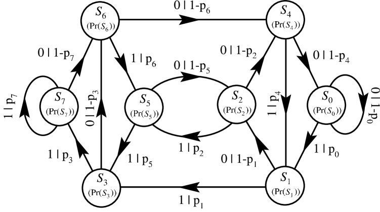
Figure 1: The most general ${r}=3$ $\epsilon$-machine. We show only the recurrent portion of the $\epsilon$-machine, as the transient part is not physically relevant (at this stage). The CSs are labeled by the last three spins seen, i.e. $S_{5}$ means that 101 were the last three spins seen. The numbers in parentheses are the asymptotic CS probabilities. The edge label $s|p$ indicates a transition on spin $s$ with probability $p$.

Now that a statistical description of the stacking process has been found in the form of an $\epsilon$-machine, it is desirable to give an intuitive notion of what the structure of the $\epsilon$-machine tells us about the patterns and disorder in a stacking process. In this section, we define and discuss architectural features of ${r}=3$ $\epsilon$-machines and their relation to the FM. Specifically, we discuss the form that growth, deformation, and layer-displacement faulting for the 2H and 3C structures assume on an ${r}=3$ $\epsilon$-machine. With this connection in place, we then address the general interpretation of $\epsilon$-machines as related to the stacking of CPSs and demonstrate the superiority of the $\epsilon$-machine as a general indicator of structure and disorder in CPSs.

III.1 Causal-State Cycles

III.1.1 Definitions

Since the $\epsilon$-machine reconstructed at ${r}$ can distinguish at most only $2^{{r}}$ pasts, it can have no more than $2^{{r}}$ CSs. The most general reconstructed $\epsilon$-machine of memory length ${r}$ is topologically equivalent to a de Bruijn graph Teubner (1990) of order ${r}$. By “most general” we mean that all length-${r}$ pasts are distinguished and all allowed transitions between CSs exist. Under these assumptions, the most general binary ${r}=3$ $\epsilon$-machine (which has $2^{3}=8$ CSs and $2^{3+1}=16$ transitions) is shown in Fig. 1. It is known that de Bruijn graphs can broken into a finite number of closed, nonself-intersecting loops called simple cycles (SCs). Canright and Watson (1996)

By analogy, we define a causal-state cycle (CSC) as a finite, closed, nonself-intersecting, symbol-specific path on an $\epsilon$-machine. We denote a CSC by the sequence of CSs visited in square brackets [ ]. The states themselves are labeled with a number (in decimal notation) that gives the sequence of the last three spins leading to that CS. For example, for an ${r}=3$ reconstructed $\epsilon$-machine, CS ${\cal S}_{3}$ means that $011$ were the last three spins observed before reaching that CS. The period of the CSC is the number of CSs that comprise it.

We further divide CSCs into strong and weak depending on the strengths of the transitions between the CSs that make up the CSC. The causal-state cycle probability ${P_{CSC}}$ is defined as the cumulative probability to complete one loop of a CSC, beginning on the CSC. We identify CSCs with large ${P_{CSC}}$ as strong CSCs and all others as weak CSCs.

[${\cal S}_{0}$]	(0)∗	3C
[${\cal S}_{7}$]	(1)∗	3C
[${\cal S}_{2}{\cal S}_{5}$]	(01)∗	2H
[${\cal S}_{1}{\cal S}_{3}{\cal S}_{6}{\cal S}_{4}$]	(0011)∗	4H
[${\cal S}_{1}{\cal S}_{3}{\cal S}_{7}{\cal S}_{6}{\cal S}_{4}{\cal S}_{0}$]	(000111)∗	6H
[${\cal S}_{5}{\cal S}_{2}{\cal S}_{4}{\cal S}_{1}{\cal S}_{3}{\cal S}_{7}$]	(001101)∗	6Ha
[${\cal S}_{2}{\cal S}_{5}{\cal S}_{3}{\cal S}_{7}{\cal S}_{4}{\cal S}_{1}$]	(110010)∗	6Ha
[${\cal S}_{5}{\cal S}_{2}{\cal S}_{4}{\cal S}_{0}{\cal S}_{1}{\cal S}_{3}{\cal S}_{7}{\cal S}_{6}$]	(00011101)∗	8Ha
[${\cal S}_{2}{\cal S}_{5}{\cal S}_{3}{\cal S}_{7}{\cal S}_{6}{\cal S}_{4}{\cal S}_{0}{\cal S}_{1}$]	(11100010)∗	8Ha
[${\cal S}_{3}{\cal S}_{6}{\cal S}_{5}$]	(011)∗	9R
[${\cal S}_{4}{\cal S}_{1}{\cal S}_{2}$]	(100)∗	9R
[${\cal S}_{7}{\cal S}_{6}{\cal S}_{5}{\cal S}_{3}$]	(0111)∗	12R
[${\cal S}_{0}{\cal S}_{1}{\cal S}_{2}{\cal S}_{4}$]	(1000)∗	12R
[${\cal S}_{3}{\cal S}_{6}{\cal S}_{4}{\cal S}_{0}{\cal S}_{1}$]	(00011)∗	15R
[${\cal S}_{4}{\cal S}_{1}{\cal S}_{3}{\cal S}_{7}{\cal S}_{6}$]	(11100)∗	15R
[${\cal S}_{5}{\cal S}_{2}{\cal S}_{4}{\cal S}_{0}{\cal S}_{1}{\cal S}_{3}{\cal S}_{6}$]	(0001101)∗	21Ra
[${\cal S}_{2}{\cal S}_{5}{\cal S}_{3}{\cal S}_{7}{\cal S}_{6}{\cal S}_{4}{\cal S}_{1}$]	(1110010)∗	21Ra
[${\cal S}_{3}{\cal S}_{6}{\cal S}_{4}{\cal S}_{0}{\cal S}_{1}{\cal S}_{2}{\cal S}_{5}$]	(0001011)∗	21Rb
[${\cal S}_{4}{\cal S}_{1}{\cal S}_{3}{\cal S}_{7}{\cal S}_{6}{\cal S}_{5}{\cal S}_{2}$]	(1110100)∗	21Rb

Table 2: The $19$ CSCs on an ${r}=3$ $\epsilon$-machine. In the first column, we give the CSC and in the second we show the stacking sequence in the Hägg notation implied by this CSC. If these CSCs are strongly represented on the $\epsilon$-machine, then we can interpret them as crystal structure. The corresponding crystal structures are shown in the third column in the Ramsdell notation. not (b) Some CSCs come in pairs related by spin-inversion symmetry, Varn and Canright (2001) i.e. [${\cal S}_{0}$] and [${\cal S}_{7}$] are both 3C structure, differing only in chirality. In cases where the Ramsdell notation is identical for different structures, we have attached a subscript to distinguish them. We list the period-$8$ hexagonal structures with a subscript to differentiate them from the more common 8H structure (00001111). One must perform $\epsilon$MSR at ${r}=4$ to discover this latter 8H structure.

III.1.2 Structural Interpretations

We begin by noting that a purely crystalline structure is simply the repetition of a sequence of MLs. This is realized on an $\epsilon$-machine as a CSC with a ${P_{CSC}}=1$. That is, an $\epsilon$-machine consisting of a single CSC repeats the same state sequence endlessly, giving a periodic stacking sequence, which physically is some crystal structure. It is therefore useful to catalog all of the possible CSCs on an ${r}=3$ $\epsilon$-machine, and this is done in Table 2. There are $19$ CSCs on an ${r}=3$ $\epsilon$-machine, and each can be thought of as a crystal structure if that CSC is strongly represented. (These should be verified by tracing them out on Fig. 1.)

However, if a nearly perfect crystal has a few randomly inserted stacking errors, these “mistakes” are physically an interruption of the regular ordering of MLs. That is, some error occurs, but after a relatively short distance the crystal returns to its regular stacking rule, thus restoring the crystalline structure. This is realized on an $\epsilon$-machine as a CSC with ${P_{CSC}}(\rm{crystal})\approx 1$ and another weakly represented CSC with ${P_{CSC}}(\rm{fault})\ll 1$. In this way, we interpret weakly represented CSCs as faults.

With this understanding in place, we note that an $\epsilon$-machine can quite naturally accommodate more than one crystal structure. Each such CSC must have a ${P_{CSC}}(\rm{crystal})\approx 1$, but they can be “connected” through a weak CSC, (${P_{CSC}}(\rm{fault})\ll 1$). However, to interpret two CSCs as crystalline structure, each must have ${P_{CSC}}(\rm{crystal})\approx 1$, and therefore necessarily they do not share a CS. (If they did, at least one CSC could not have a ${P_{CSC}}(\rm{crystal})\approx 1$.) Similarly, $\epsilon$-machines can accommodate more that one faulting structure.

III.2 Faulting Structures on $\epsilon$-Machines

As we did with crystal structures on an ${r}=3$ $\epsilon$-machine, it is instructive to identify some of the more common faults on the most general ${r}=3$ $\epsilon$-machine. We will consider only 2H and 3C structures with growth, deformation, and layer-displacement faults; but the extension to other crystal and fault structures is straightforward. We will only give the faulting structure on an $\epsilon$-machine to first order in the faulting probability, so that the basic graphical structure is clear. Thus, the connection with the FM is valid only for weak faulting; which is consistent with the FM’s domain of applicability. The $\epsilon$-machine, however, is valid for any degree of disorder, it is only the connection to the FM that is limited to weak faulting.

We also note that the faults on the $\epsilon$-machine in this interpretation are such that the occurrence of two adjacent faults is suppressed. If the probability of encountering a fault on a ML is (say) $p$, then the probability of two adjacent faults is $p^{2}$. That is, in our attempt to use the FM to interpret the structures captured by an $\epsilon$-machine, we ignore these higher-order terms. Thus, the issue of random versus nonrandom faulting in polytypism is not addressed here. But, again, we note that the $\epsilon$-machine description quite naturally describes random, nonrandom, and periodic faulting structures. Sebastian and Krishna (1994)

III.2.1 Growth Faults

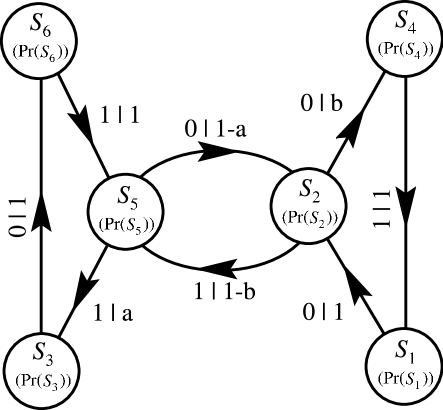
Figure 2: Growth faults for the 2H structure as they appear on a ${r}=3$ $\epsilon$-machine for small faulting probabilities $a$ and $b$. The [${\cal S}_{2}{\cal S}_{5}$] CSC is the 2H structure and the CSCs [${\cal S}_{5}{\cal S}_{3}{\cal S}_{6}$] and [${\cal S}_{2}{\cal S}_{4}{\cal S}_{1}$] give the faulting. This interpretation is only valid for small faulting probabilities.

Crystal growth often proceeds by a layer-addition process. Suppose a ML is added that cannot be thought of as a continuation of the previous crystal structure, but the MLs added subsequent to that ML return to the original stacking rule. Such a ML inserted into the sequence is called a growth fault. For the 2H structure, the rule is that the added ML has the same orientation as the next-to-last ML. For example, imagine an unfaulted 2H crystal, consisting of $A$ and $B$ MLs, is $...ABABAB...$. Then a growth fault in this structure is a $B$ ML followed by a $C$ ML. The remaining MLs continue to follow the 2H stacking rule, giving an overall stacking sequence such as

$$...A\>B\>A\>B\>A\>B\>\underline{C}\>B\>C\>B\>C\>B...~{},$$

where underlining indicates the fault plane.

Notice that the original crystal is composed of alternating $A$ and $B$ MLs, while after the fault it becomes a sequence of alternating $B$ and $C$ MLs. In terms of the Hägg notation, a growth fault for the 2H crystal corresponds to the insertion of a single $0$ or $1$ into the spin sequence. For example, $...01010101...$ becomes $...0101\underline{1}0101...$ upon insertion of a $1$, where the underlining indicates the inserted spin.

This can be demonstrated on the $\epsilon$-machine shown in Fig. 2 with small faulting probabilities $a$ and $b$. This $\epsilon$-machine implies that the CSC represented by [${\cal S}_{2}{\cal S}_{5}$] is dominant, which is simply the 2H structure. With small faulting probabilities $a$ or $b$, a $0$ or a $1$, respectively, is randomly inserted into the 2H crystalline structure.

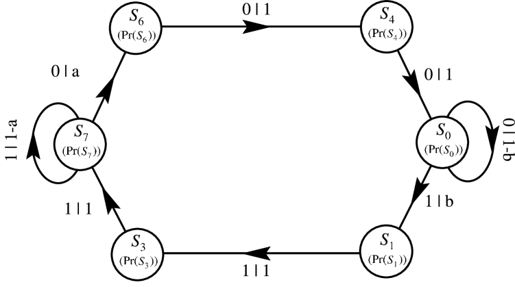
Figure 3: Growth faults for the 3C structure on a ${r}=3$ $\epsilon$-machine with small faulting probabilities $a$ and $b$. The CSCs [${\cal S}_{7}$] and [${\cal S}_{0}$] give the twinned 3C structure, while the paths ${\cal S}_{7}{\cal S}_{6}{\cal S}_{4}{\cal S}_{0}$ and ${\cal S}_{0}{\cal S}_{1}{\cal S}_{3}{\cal S}_{7}$ give the faulting. Here we have an example of a faulting structure that induces a transition between two crystal structures.

In the 3C structure, the stacking rule is that the added ML is different from the previous two MLs. There are, of course, two distinct, symmetry-related 3C structures; one being the $...ABCABC...$ and the other its spatial inversion $...CBACBA...$. The spin sequences for these are $...1111...$ and $...0000...$, respectively. A growth fault for this crystal gives a stacking sequence such as

$$...A\>B\>C\>A\>B\>\underline{C}\>B\>A\>C\>B\>A...~{},$$

where underlining again indicates the fault plane. It is conventional to take the indicated ML as the fault plane since it is the only ML in the cubic stacking sequence that is hexagonally related to its neighbors. In terms of Hägg notation, the sequence is $...11111|00000...$, where the vertical line indicates the fault plane. The effect of a growth fault in a 3C structure is then to switch from 3C structure of one chirality to another or to flip all spins after the fault plane. This fault is also known as a twin fault of the 3C structure, because it produces a crystal containing both kinds of 3C sequences. This growth fault is demonstrated in Fig. 3 with small faulting probabilities $a$ and $b$. The two CSCs [${\cal S}_{7}$] and [${\cal S}_{0}$] correspond to the two twinned 3C structures, with the transition sequences connecting them having a small total probability.

III.2.2 Deformation Faults

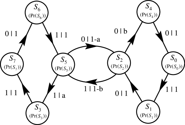
Figure 4: Deformation faulting for the 2H structure on a ${r}=3$ $\epsilon$-machine for small fault probabilities $a$ and $b$. A deformation fault is represented by a single spin flip.

Other faults can occur after a crystal structure has been formed. Caused by external stresses or inhomogeneous temperature distributions within the crystal, deformation faults are the result of one plane in the crystal slipping past another in a direction transverse to the stacking. An example of deformation faulting in the 2H structure is the following:

$$...A\>B\>A\>B\>|\>C\>A\>C\>A\>C\>A...~{}.$$

The vertical bar indicates the plane across which the slip occurred. In the Hägg notation a deformation fault in the 2H structure is realized by flipping a spin. In this example, the unfaulted sequence …10101010… transforms to …10111010…, where again the underlined spin demarcates the one flipped. The $\epsilon$-machine representation of this fault is shown in Fig. 4.

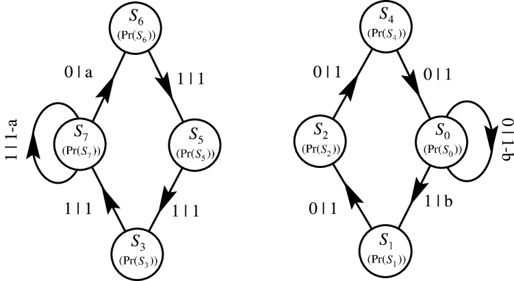
Figure 5: The two possible $\epsilon$-machines for deformation faulting in the 3C structure with small faulting probabilities $a$ and $b$. There are two $\epsilon$-machines, one for faulting from each of the 3C structures, [${\cal S}_{7}$] and [${\cal S}_{0}$]. They are disconnected, and hence faulting in the 3C structure of one chirality cannot cause the crystal to switch to another chirality. Hence this faulting mechanism does not cause twinning.

In the 3C structure, deformation faults appear much the same. An example of a deformation fault in a 3C structure is

$$...A\>B\>C\>A\>B\>C\>|\>B\>C\>A\>B\>C\>A...$$

The vertical bar again indicates the slip plane. Expressed in spin notation, the unfaulted 3C crystal $...11111111...$ becomes $...1111\underline{0}111...$, a single spin flip. The two corresponding $\epsilon$-machines are shown in Fig. 5.

III.2.3 Layer-Displacement Faults

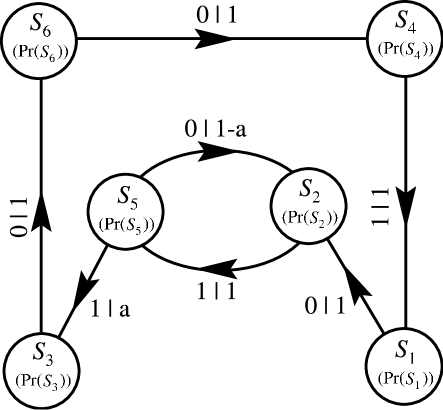
Figure 6: Layer-displacement faults for the 2H structure on a ${r}=3$ $\epsilon$-machine with small faulting probability $a$. Here, for the sake of clarity, we show only faulting initiating from the ${\cal S}_{5}$ CS, although a similar faulting structure can begin from the ${\cal S}_{2}$ CS.

Layer-displacement faults are characterized by a shifting of one or two MLs in the crystal, while leaving the remainder of the crystal undisturbed. As such, these faults do not disrupt the long-range order present in a structure. They are thought to be introduced at high temperatures by diffusion of the atoms through the crystal. Sebastian and Krishna (1994) In the 2H structure, an example of a layer-displacement fault is:

$$...A\>B\>A\>B\>\underline{C}\>B\>A\>B\>A...~{},$$

where the underlined ML is the faulted layer. Written as spins, $...10101010...$ becomes $...101\underline{10}010...$, the underlined spins indicating those that have flipped. A layer-displacement fault in the 2H structure is shown in Fig. 6.

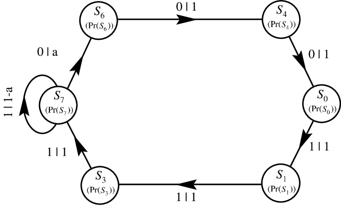
Figure 7: Layer-displacement faults for the 3C structure on a ${r}=3$ $\epsilon$-machine with small faulting probability $a$. Again, we show only faulting from the ${\cal S}_{7}$ CS, corresponding to the $...1111...$ spin sequence. A similar fault structure could be drawn for faulting from the ${\cal S}_{0}$ CS. A layer-displacement fault for the 3C structure is achieved by three consecutive spin flips. The difference between the fault structure here and that of a growth fault for the 3C structure is that growth faults produce twinning, whereas here the fault returns to the original crystal structure.

Layer-displacement faults in 3C structures are more difficult to realize, since each ML is sandwiched between two unlike MLs and changing its orientation violates the stacking constraints. It is therefore necessary for two adjacent MLs to shift. Consequently, one expects that they are rarer. An example of layer-displacement in the 3C structure is the following:

$$\ldots A\>B\>C\>A\>B\>C\>\underline{B\>A}\>C\>A\>B\>C\>AB\>\ldots~{},$$

where the underlined layers are faulted. The spin sequence changes from $\ldots 1111111\ldots$ to one where three consecutive spins have been flipped to $0$: $\ldots...1100011\ldots$. A layer-displacement fault on the 3C structure is shown in Fig. 7.

These common faulting structures for the 2H and 3C crystals are given in Table 3 along with the CSCs associated with them.

2H	Growth fault	${\cal S}_{5}{\cal S}_{3}{\cal S}_{6}$
		${\cal S}_{2}{\cal S}_{4}{\cal S}_{1}$
	Deformation fault	${\cal S}_{5}{\cal S}_{3}{\cal S}_{7}{\cal S}_{6}$
		${\cal S}_{2}{\cal S}_{4}{\cal S}_{0}{\cal S}_{1}$
	Layer-displacement fault	${\cal S}_{5}{\cal S}_{3}{\cal S}_{6}{\cal S}_{4}{\cal S}_{1}{\cal S}_{2}$
		${\cal S}_{2}{\cal S}_{4}{\cal S}_{1}{\cal S}_{3}{\cal S}_{6}{\cal S}_{5}$
3C	Growth fault	${\cal S}_{7}{\cal S}_{6}{\cal S}_{4}{\cal S}_{0}$
		${\cal S}_{0}{\cal S}_{1}{\cal S}_{3}{\cal S}_{7}$
	Deformation fault	${\cal S}_{7}{\cal S}_{6}{\cal S}_{5}{\cal S}_{3}$
		${\cal S}_{0}{\cal S}_{1}{\cal S}_{2}{\cal S}_{4}$
	Layer-displacement fault	${\cal S}_{7}{\cal S}_{6}{\cal S}_{4}{\cal S}_{0}{\cal S}_{1}{\cal S}_{3}$
		${\cal S}_{0}{\cal S}_{1}{\cal S}_{3}{\cal S}_{7}{\cal S}_{6}{\cal S}_{4}$

Table 3: The more common fault structures for the 2H and 3C structures on an ${r}=3$ $\epsilon$-machine. We make the following interpretation: If there is one parent structure (2H or 3C) that is strongly represented and a single additional CSC is associated with it as shown above, then we say that that crystal has the structure of the parent crystal with a certain amount of the given faulting. We should be clear here, however, not to confuse structure with mechanism. In this interpretation, the $\epsilon$-machine gives the structure that a crystal would have if it experienced a small amount of the faulting given. Structure does not necessarily imply mechanism.

III.3 $\epsilon$-Machine Decomposition and General Interpretation

The previous discussion has emphasized the important rôle that CSCs play in reflecting stacking structures—crystalline and fault. We have found that CSCs directly correspond to crystal and fault structures. The question then arises, can any arbitrary ${r}=3$ $\epsilon$-machine be decomposed into crystal and fault structures? We first note that the only difference between fault and crystal structure is the magnitude of the ${P_{CSC}}$ associated with each CSC. It seems reasonable, then, to break an $\epsilon$-machine into a sum of CSCs. So we formally write,

$$\mathcal{E}\sim\sum_{i}\nu_{i}(CSC_{i})~{},$$ (24)

where $\mathcal{E}$ is the $\epsilon$-machine, $\nu_{i}$ is the fraction of the $\epsilon$-machine that can be attributed to the $i^{\mathrm{th}}$ CSC, and $CSC_{i}$ is the $i^{\mathrm{th}}$ CSC. The most general binary ${r}=3$ $\epsilon$-machine can be specified by eight variables. It is known, however, that there are $19$ CSCs on such an $\epsilon$-machine. Teubner (1990) So, unless there is a fortuitous vanishing of either CSs or $\epsilon$-machine transitions, or the imposition of additional constraints, the decomposition in Eq. (24) is not unique and therefore of questionable use. We note this situation is not expected to improve with larger ${r}$. The number of parameters on the ${r}^{\mathrm{th}}$ $\epsilon$-machine grows exponentially in ${r}$, while the number of CSCs appears to increase as the exponential of an exponential in ${r}$. Teubner (1990) Thus, in general, it is not possible to decompose an $\epsilon$-machine into CSCs uniquely.

The main purpose of such a decomposition is to provide intuition into the structure present and possibly insight into the physical mechanisms that may have led to a particular structure. In this limited capacity Eq. (24) may be helpful. We stress that Eq. (24) has no other use than this and certainly cannot be used to calculate physical quantities. Only the entire $\epsilon$-machine is suitable for such calculations.

How, then do we intuitively understand structure on an $\epsilon$-machine? In one picture—the weak faulting limit—we view the $\epsilon$-machine as a collection of CSCs. The decomposition given by Eq. (24), while not unique, may be sensible. In this case, we have the same interpretation as the FM. However, the $\epsilon$-machine has a broader range of applicability. It can, for instance, accommodate more than one crystal structure and detail how the stacking alternates between the two. The FM, to our knowledge, admits no such multicrystalline structures. The $\epsilon$-machine provides a more detailed account of multiple faulting structures. The FM, too, can reflect more than one kind of faulting structure, but the description is a stochastic one. The $\epsilon$-machine has no difficulty in reflecting any stacking structures, even closely spaced faulting structures. Thus, we retain the structural interpretations of §III.1.2 for the case of weakly faulted structures.

In other circumstances, when a sensible decomposition of the $\epsilon$-machine into crystal and faulting structures is not possible, it still gives insight into important stacking sequences and their spatial relations. Although it is no longer as advantageous to view the $\epsilon$-machine as a collection of CSCs, we note that stacking sequence probabilities are readily observed on the $\epsilon$-machine either through direct calculation—the $\epsilon$-machine specifies sequence frequencies of any length—or, more simply for shorter sequences, by asymptotic CS probabilities. The likelihood of seeing two sequences in close proximity can be found by tracing the appropriate path through the $\epsilon$-machine. Since the $\epsilon$-machine is valid for any degree of disorder, we can find the relative importance of stacking sequences for even heavily faulted crystals or for crystals in which no regular stacking structures exist. The architecture of the $\epsilon$-machine—i.e., the number, arrangement, and connections between the CSs, then provides an intuitive interpretation for the complexity and organization of the structure. One sees how the various stacking structures are related and how one blends into another upon scanning the crystal.

Thus, in addition to providing a formidable calculational tool, the $\epsilon$-machine provides a new way of viewing structure in layered materials; it is not tethered to the assumption of a parent crystal permeated with weak faults. It gives a generalized way to view and compare the structure of different crystals, even when they have different—or no—parent structures. This should prove especially helpful in understanding solid-state transformations in layered materials, as we intend to demonstrate in follow-on work.

Finally, we note that these are interpretations of convenience, not necessity. The $\epsilon$-machine is a unique description of the stacking process, and thus any quantities that depend directly on a statistical description of the stacking are amenable to calculation.

For those instances where a sensible decomposition of the $\epsilon$-machine is possible—i.e., the weak faulting limits—we employ Eq. (24) for the limited purpose of providing an intuitive understanding of the disordered structure We will call $\nu_{i}$ either the fraction of crystal structure or, for weak CSCs, the fault density. This is, of course, different from the fault probability generally used in the literature. The fault probability is the frequency, upon scanning the stacking sequence, that one finds a particular fault in the sequence.

IV Example Processes

We consider four prototype processes to demonstrate $\epsilon$MSR. In Example A, we reconstruct an $\epsilon$-machine for a known ${r}=3$ process and show that the technique works in this case and, indeed, for any process that has ${r}_{l}\leq 3$. In Example B, we consider a process that cannot be represented on a ${r}=3$ $\epsilon$-machine. We reconstruct an $\epsilon$-machine for a process that requires a ${r}_{l}=4$ memory length and find that a ${r}=3$ $\epsilon$-machine gives a reasonable approximation. In Example C, we treat a process with ${r}_{l}=1$ to demonstrate that $\epsilon$MSR does terminate at the minimum ${r}$. We also show that had we not terminated reconstruction at ${r}=1$, the equivalence relation, Eq. (11) would require the merging of equivalent histories that would effectively find the ${r}=1$ $\epsilon$-machine. Finally, in Example D, we reconstruct the ${r}=3$ $\epsilon$-machine for the even process—a finite-state process that has a distinctive kind of infinite memory. Crutchfield and Feldman (2003); Crutchfield (1992) Again, we find that the ${r}=3$ $\epsilon$-machine gives a reasonable approximation.

In Examples A, B, and D, we solve the spectral equations at ${r}=3$ with the memory-length reduction approximation via a Monte Carlo technique. Varn (2001) These equations are given in Appendix A. To find the predicted CFs for each $\epsilon$-machine, we take a sample spin sequence generated by the $\epsilon$-machine of length 400 000 and find the CFs by directly scanning the resulting stacking sequence. The diffraction spectra are calculated from Eq. (1) using a sample of 10 000 MLs. Since these are theoretical spectra, and have no error, we are not able to set an acceptable threshold error in advance. Instead, we have chosen examples, except for Example C, that require the ${r}=3$ solutions and we solve these examples at ${r}=3$. In the event that a CS is assigned an asymptotic state probability of less than $0.01$, we take that CS to be nonexistent.

We also calculate the information-theoretic quantities described in §II.7 for each example and the reconstructed $\epsilon$-machine and display the results in Table 7. Analyzing these examples not only demonstrates the feasibility and accuracy of spectral $\epsilon$-machine reconstruction, but they also serve to illustrate how $\epsilon$-machines capture structure and disorder. In the companion sequel, Varn et al. (2002b) we apply the same procedures to the analysis of experimental diffraction spectra from ZnS, focusing on the novel physical and material properties that can be discovered with this technique.

IV.1 Example A

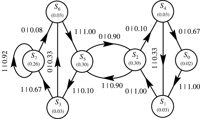
Figure 8: The ${r}=3$ $\epsilon$-machine for the Example A process. The asymptotic probabilities are given for each CS. The large CSC probabilities for the [${\cal S}_{7}$] CSC (${P_{CSC}}([{\cal S}_{7}])=0.92$) and the [${\cal S}_{2}{\cal S}_{5}$] CSC (${P_{CSC}}[{\cal S}_{2}{\cal S}_{5}])=0.81$) suggest that one think of these cycles as crystal structure and everything else as faulting.

Figure 9: A comparison between the diffraction spectra $\mathsf{I}(l)$ generated by Example A and by the ${r}=3$ spectrally reconstructed $\epsilon$-machine. The differences between the diffraction spectra for Example A and the ${r}=3$ reconstructed $\epsilon$-machine are too small to be seen. We calculate ${\cal R}=2\%$, but this is largely due to numerical error. (See text.) The peak at $l\approx 1/3$ corresponds to the 3C structure and the two peaks at $l\approx 1/2$ and $l\approx 1$ to the 2H structure.

We begin with the sample process given in Fig. 8. This process can approximately be decomposed into FM structural components using Eq. (24) in the following way:

$\begin{array}[]{lr}\textrm{2H}&$ 54\% $\\ \textrm{3C${}^{+}$}&$ 24\% $\\ \textrm{Deformation fault}&$ 16\% $\\ \textrm{Growth fault}&$ 6\% $\end{array}$

where the “+” on 3C indicates that only the positive chirality ($...1111...$) structure is present. The faulting is given with reference to the 2H crystal.

The diffraction spectrum from this process is shown in Fig. 9. The experienced crystallographer has little difficulty guessing the underlying crystal structure: the peaks at $l\approx 1/2$ and at $l\approx 1$ suggest the 2H structure; while the peak at $l\approx 1/3$ is characteristic of the 3C structure.

The mechanism responsible for the faulting is less clear, however. It is known that various kinds of fault produce different effects on the Bragg peaks. Sebastian and Krishna (1994) For instance, both growth and deformation faults broaden the peaks in the diffraction spectrum of the 2H structure, the difference being that growth faults broaden the integer-$l$ peaks three times more than the half-integer-$l$ peaks, while broadening due to deformation faulting is about equal. The FWHM for the peaks are $0.028$, $0.034$, and $0.049$ for $l\approx 0.33$, $0.5$, and $1$, respectively. This gives then a ratio of about $1.4$ for the integer-$l$ to half-integer-$l$ broadening, suggesting (perhaps) that deformation faulting is prominent. One expects there to be no shift in the position of the peaks for either growth or deformation faulting; which is clearly not the case here. In fact, the two peaks associated with the 2H structure at $l\approx 0.5$ and 1 are shifted by $\Delta l\approx 0.006$ and 0.009, respectively. This analysis is, of course, only justified for one parent crystal in the overall structure, nonetheless if we neglect the peak shifts, the simple intuitive analysis appears to give good qualitative results here.

With the 3C peak, both deformation and growth faults produce a broadening, the difference being that the broadening is asymmetrical for the growth faults. One also expects there to be some peak shifting for the deformation faulting. There is a slight shift ($\Delta l\approx 0.002$) for the $l\approx 1/3$ peak and the broadening seems (arguably) symmetric, so one is tempted to guess that deformation faulting is important here. Indeed, the CSC [${\cal S}_{7}{\cal S}_{6}{\cal S}_{5}{\cal S}_{3}$] is consistent with deformation faulting in the 3C crystal. Heuristic arguments, while not justified here, seem to give qualitative agreement with the known structure.

Figure 10: A comparison of the CFs $Q_{s}(n)$ between the Example A process and the ${r}=3$ reconstructed $\epsilon$-machine. As with the diffraction spectra, the differences are too small to be seen on the graph. As an aid to the eye, here and in other graphs showing CFs, we connect the the values of adjacent CFs with straight lines. The CFs, of course, are defined only for integer values of $n$.

The $\epsilon$-machine description does better. We follow the spectral reconstruction procedure given in §II. We Fourier analyze the spectrum over the interval $0\leq l\leq 1$. The figures-of-merit are equal to their theoretical values within numerical error. The reconstructed $\epsilon$-machine is equivalent to the original one, with CS probabilities and transition probabilities typically within 0.1% of their original values, except for the transition $1|0.33$ from ${\cal S}_{4}$, which was 1% too small. Not surprisingly, the process shown in Fig. 8 is the reconstructed $\epsilon$-machine and so we do not repeat the figure.

The two-layer CFs $Q_{s}(n)$ versus $n$ from the process and from the reconstructed $\epsilon$-machine are shown in Fig. 10. The differences are too small to be seen on the graph. We calculate the profile $\cal R$-factor to compare the “experimental” spectrum (Example A) to the “theoretical” spectrum ($\epsilon$-machine) and find a value of ${\cal R}\approx 2\%$. If we generate several spectra from the same process, we find profile $\cal R$-factors of similar magnitude. This error is then must be due to sampling. It stems from the finite spin sequence length we use to calculate the CFs and our method for setting them equal to their asymptotic value. (See §II.2.) This can be improved by taking longer sample sequence lengths and refining the procedure for setting the CFs to their asymptotic value. Since typical profile $\cal R$-factors comparing theory and experiment are much larger than this, at present, this does not seem problematic. A comparison of the two spectra is shown in Fig. (9). This kind of agreement is typical of spectral $\epsilon$-machine reconstruction from any process that can be represented as a ${r}=3$ $\epsilon$-machine. Varn (2001)

We find by direct calculation from the $\epsilon$-machine that both Example A and the reconstructed process have a configurational entropy of ${h_{\mu}}\approx 0.44$ bits/spin, a statistical complexity of ${C_{\mu}}\approx 2.27$ bits, and an excess entropy of ${\bf E}\approx 0.95$ bits.

Since the original process was representable as an $r=3$ $\epsilon$-machine, this first example is largely a consistency check on $\epsilon$MSR. In the next example, we treat an ${r}>3$ process not representable by the ${r}=3$ $\epsilon$-machines that we reconstruct.

IV.2 Example B

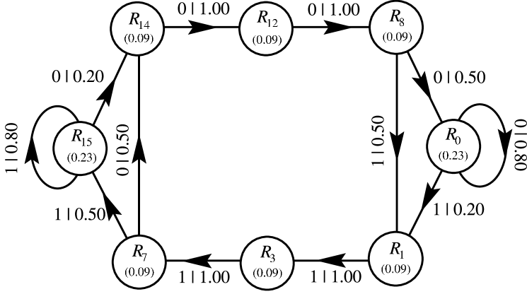
Figure 11: The process for Example B. Since it has a memory of ${r}_{l}=4$, we label the states with the last four spins observed: i.e., $\mathcal{R}_{12}$ means that $1100$ were the last four spins. The CSCs [$\mathcal{R}_{15}$] and [$\mathcal{R}_{0}$] give rise to 3C structure and the CSC [$\mathcal{R}_{1}\mathcal{R}_{3}\mathcal{R}_{7}\mathcal{R}_{14}\mathcal{R}_{12}\mathcal{R}_{8}$] generates 6H structure.

Upon annealing, a solid-state transformation in ZnS from the 2H structure to either the 3C or 6H structures is possible, sometimes both occurring in different parts of the same crystal. Sebastian and Krishna (1994) However, two crystal structures represented with an $\epsilon$-machine cannot share a CS, as discussed in §III.1.2. On a ${r}=3$ $\epsilon$-machine, for example, both the CSCs associated with the 3C and the 6H structures share the CSs ${\cal S}_{7}$ and ${\cal S}_{0}$, so a crystal containing both structures cannot be properly modeled at ${r}=3$. In fact, it is necessary to use an ${r}=4$ $\epsilon$-machine to encompass both structures. So, to see how well spectral reconstruction works at ${r}=3$ for an ${r}=4$ process, we consider the process shown in Fig. 11. The CSC [$\mathcal{R}_{1}\mathcal{R}_{3}\mathcal{R}_{7}\mathcal{R}_{14}\mathcal{R}_{12}\mathcal{R}_{8}$] would give rise to 6H structure if it were a strong CSC, but we find that $P_{6H}=0.25$. We say then that this is mild 6H structure. The CSCs [$\mathcal{R}_{0}$] and [$\mathcal{R}_{15}$] give the twinned 3C structures.

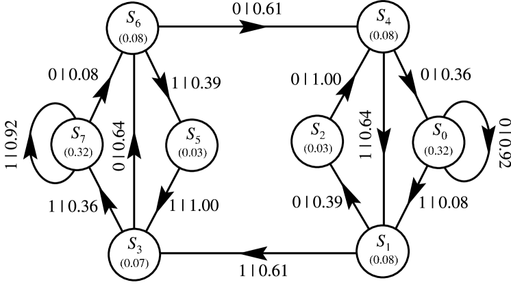
Figure 12: The $\epsilon$-machine reconstructed at ${r}=3$ for Example B.

The figures of merit were all equal to their theoretical values within numerical error. Employing spectral reconstruction, we find the ${r}=3$ $\epsilon$-machine shown in Fig. 12. All CSs are present and all transitions, save those that connect the ${\cal S}_{2}$ and ${\cal S}_{5}$ CSs, are present. A comparison of the CFs for the original process and the reconstructed $\epsilon$-machine is given in Fig. 13. The agreement is remarkably good. It seems that the ${r}=3$ $\epsilon$-machine picks up most of the structure in the original process.

There is similar, though not as good, agreement in the diffraction spectra, as Fig. 14 shows. The most notable discrepancies are in the small rises at $l\approx 1/6$ and $l\approx 5/6$. We calculate a profile ${\cal R}$-factor of ${\cal R}=12\%$ between the diffraction spectra for Example B and the reconstructed $\epsilon$-machine. The ${r}=3$ $\epsilon$-machine has difficulty reproducing the 6H structure in the presence of 3C structure, as expected.

Figure 13: A comparison of the CFs $Q_{s}(n)$ generated by the ${r}=3$ reconstructed $\epsilon$-machine (dashed line) and generated by Example B (solid line). The agreement is excellent.

Given the good agreement between the correlation functions and the spectra generated by Example B and the ${r}=3$ $\epsilon$-machine, we are led to ask what the differences between the two are. In Table 4 we give the frequencies of the eight length-3 sequences generated by each process. The agreement is excellent. They both give the same probabilities for the most common length-$3$ sequences, $111$ and $000$. Example B does forbid two length-$3$ sequences, $101$ and $010$, which the reconstructed ${r}=3$ $\epsilon$-machine allows with a small probability (0.03). At the level of length-$3$ sequences, the $\epsilon$-machine is capturing most of the structure in the stacking sequence.

A similar analysis allows us to compare the probabilities of the $16$ length-$4$ sequences generated by each; the results are given in Table 5. There are more striking differences here. The frequencies of the two most common length-4 sequences in Example B, ${\rm P}(1111)={\rm P}(0000)=0.23$, are overestimated by the ${r}=3$ $\epsilon$-machine, which assigns them a probability of $0.29$ each. Similarly, sequences forbidden by Example B—$1101$, $1011$, $1010$, $1001$, $0110$, $0101$, $0100$, $0010$—are not necessarily forbidden by the ${r}=3$ $\epsilon$-machine. In fact, the ${r}=3$ $\epsilon$-machine forbids only two of them, $0101$ and $1010$. This implies that ${r}=3$ $\epsilon$-machine can find spurious sequences that are not in the original stacking sequence. This is to be expected. But the ${r}=3$ $\epsilon$-machine does detect important features of the original process. It finds that this is a twinned 3C structure. It also finds that 2H structure plays no role in the stacking process. (We see this by the absence of transitions between the ${\cal S}_{2}$ and ${\cal S}_{5}$ CSs in Fig. 12.)

One can also attempt to decompose the ${r}=3$ $\epsilon$-machine into a sum of CSCs and interpret this as crystal and fault structure. However, as is typically the case, there is no unique decomposition and so therefore such an exercise is of questionable validity. With the exception of the sequences $1111$ and $0000$, the other twelve nonvanishing sequences all appear with a small, but rather constant probability of $0.03$ or $0.05$. One possible interpretation is to say that the CSCs [${\cal S}_{0}$] and [${\cal S}_{7}$] contribute to 3C structure with a weight of $0.58$. We could further interpret the [${\cal S}_{7}{\cal S}_{6}{\cal S}_{5}{\cal S}_{3}$] and [${\cal S}_{0}{\cal S}_{1}{\cal S}_{2}{\cal S}_{4}$] CSCs as deformation faulting of the 3C structure giving a combined weight of $0.24$. And finally, we could associate the CSC [${\cal S}_{1}{\cal S}_{3}{\cal S}_{6}{\cal S}_{4}$] with 4H structure. This last interpretation of the CSC [${\cal S}_{1}{\cal S}_{3}{\cal S}_{6}{\cal S}_{4}$] with any crystal structure is troublesome as the $P_{CSC}\ll 1$. Another possible decomposition would be to again assign the CSCs [${\cal S}_{7}$] and [${\cal S}_{7}$] to the 3C structure with a weight of 0.58, to interpret the paths ${\cal S}_{7}$${\cal S}_{6}$${\cal S}_{4}$${\cal S}_{0}$ and ${\cal S}_{0}$${\cal S}_{1}$${\cal S}_{3}$${\cal S}_{7}$ as as twin faulting with a probability weight of $0.18$, treat the CSC [${\cal S}_{1}{\cal S}_{3}{\cal S}_{6}{\cal S}_{4}$] as 4H structure, and finally to interpret the two CSCs [${\cal S}_{1}{\cal S}_{2}{\cal S}_{4}$] and [${\cal S}_{3}{\cal S}_{6}{\cal S}_{5}$] as 9R structures. These two descriptions are clearly rather different and, arguably, have no use in any account, other than serving to illustrate the ambiguity of FM-like structural interpretations.

In addition to the nonuniqueness difficulties, by simply listing the probability density of the various crystals and fault structures, we say nothing about how one crystal converts into another as one scans the stacking sequence. This exercise demonstrates the impoverished view of crystal structure inherent in the FM. In short, the stacking sequence implied by the $\epsilon$-machine in Fig. 12 comes from a physical structure that is not describable in terms of the FM.

Figure 14: A comparison of the diffraction spectra $\mathsf{I}(l)$ between ${r}=3$ reconstructed $\epsilon$-machine and the process of Example B. The agreement is surprisingly good. The small peaks at $l\approx 1/6$ and $l\approx 5/6$ correspond to the 6H structure. The ${r}=3$ $\epsilon$-machine has difficulty in reproducing these because the 6H and the 3C structure both share the ${\cal S}_{7}$ and ${\cal S}_{0}$ CSs and so require an $\epsilon$-machine reconstructed at ${r}=4$ to properly disambiguate them.

Sequence	Example B	$\epsilon$MSR	Sequence	Example B	$\epsilon$MSR
111	0.32	0.32	011	0.09	0.07
110	0.09	0.07	010	0.00	0.03
101	0.00	0.03	001	0.09	0.08
100	0.09	0.08	000	0.32	0.32

Table 4: The frequencies of length-3 sequences obtained from the Example B and the $\epsilon$-machine reconstructed at ${r}=3$.

Sequence	Example B	$\epsilon$MSR	Sequence	Example B	$\epsilon$MSR
1111	0.23	0.29	0111	0.09	0.03
1110	0.09	0.03	0110	0.00	0.04
1101	0.00	0.03	0101	0.00	0.00
1100	0.09	0.04	0100	0.00	0.03
1011	0.00	0.03	0011	0.09	0.05
1010	0.00	0.00	0010	0.00	0.03
1001	0.00	0.05	0001	0.09	0.03
1000	0.09	0.03	0000	0.23	0.29

Table 5: The frequencies of length-4 sequences obtained from the Example B and the $\epsilon$-machine reconstructed at ${r}=3$.

We find by direct calculation that the Example B process has a configurational entropy of ${h_{\mu}}=0.51$ bits/spin, a statistical complexity of ${C_{\mu}}=2.86$ bits, and an excess entropy of ${\bf E}=0.82$ bits. The reconstructed process gives similar results with a configurational entropy ${h_{\mu}}=0.54$ bits/spin, a statistical complexity of ${C_{\mu}}=2.44$ bits, and an excess entropy of ${\bf E}=0.83$ bits.

IV.3 Example C

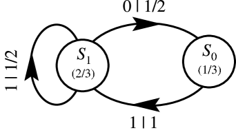
Figure 15: The recurrent portion of the $\epsilon$-machine for the golden mean process, Example C. The process has a memory length of ${r}=1$, and so we label each CS by the last spin seen.

We treat this next system, Example C, to contrast it with the last and to demonstrate how pasts with equivalent futures are merged to form CSs. The $\epsilon$-machine for this system is shown in Fig. 15 and is known as the golden mean process. The rule for generating the golden mean process is simply stated: a 0 or 1 are allowed with equal probability unless the previous spin was a 0, in which case the next spin is a $1$. Clearly then, this process needs to only remember the previous spin, and hence it has a memory length of ${r}=1$. It forbids the sequence 00 and all sequences that contain this as a subsequence. The process is so-named because the total number of allowed sequences grows with sequence length at a rate given by the golden mean $\phi=(1+\sqrt{5})/2$.

We employ the $\epsilon$MSR algorithm and find the $\epsilon$-machine given (again) in Fig. 15 at ${r}=1.$ A comparison of the CFs from Example C and the golden mean process are given in Fig. 16. The differences are too small to be seen. We next compare the diffraction spectra, and these are shown in Fig. 17. We find excellent agreement and calculate a profile ${\cal R}$-factor of ${\cal R}=2\%$. At this point $\epsilon$MSR should terminate, as we have found satisfactory agreement (to within the numerical error of our technique) between “experiment”, Example C, and “theory”, the reconstructed $\epsilon$-machine.

Figure 16: A comparison of the CFs $Q_{s}(n)$ generated by the ${r}=1$ reconstructed $\epsilon$-machine and the golden mean process of Example C. The CFs decay quickly to their asymptotic value of $1/3$.

Figure 17: A comparison of the diffraction spectra for Example C and the reconstructed ${r}=1$ $\epsilon$-machine. The agreement is excellent. One finds a profile ${\cal R}$-factor of 2% between the “experimental” spectrum, Example C, and the “theoretical” spectrum calculated from the reconstructed $\epsilon$-machine.

Let us suppose that instead, we increment ${r}$ and follow the $\epsilon$MSR algorithm as if the agreement at ${r}=1$ had been unsatisfactory. In this case, we would have generated the “$\epsilon$-machine” shown in Fig. 18 at the end of step 3b. We have yet to apply the equivalence relation Eq. (11) and so let us call this the nonminimal $\epsilon$-machine. That is, we have not yet combined pasts with equivalent futures to form CSs, step 3c. Let us do that now.

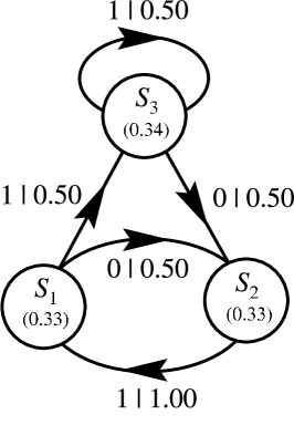
Figure 18: The ${r}=2$ reconstructed nonminimal $\epsilon$-machine for the golden mean process, Example C.

We observe that the state ${\cal S}_{2}$ is different from the other two, ${\cal S}_{1}$ and ${\cal S}_{3}$, in that one can only see the spin $1$ upon leaving this state. Therefore it cannot possibly share the same futures as ${\cal S}_{1}$ and ${\cal S}_{3}$, so no equivalence between them is possible. However, we do see that ${\rm P}(1|{\cal S}_{1})={\rm P}(1|{\cal S}_{3})=1/2$ and ${\rm P}(0|{\cal S}_{1})={\rm P}(0|{\cal S}_{3})=1/2$ and, thus, these states share the same probability of seeing futures of length-$1$. More formally, we can write

$${\sf T}_{01\rightarrow 1s}^{(s)}={\sf T}_{11\rightarrow 1s}^{(s)}~{}.$$ (25)

Since we are labeling the states by the last two symbols seen at ${r}=2$, within our approximation they do have the same futures and thus ${\cal S}_{1}$ and ${\cal S}_{3}$ can be merged to form a single CS. The result is the $\epsilon$-machine shown in Fig. 15.

In general, in order to merge two histories, we check that each has an equivalent future up to the memory length ${r}$. In this example, we need only check futures up to length-$1$, because after the addition of one spin ($s$) each is labeled by the same past, namely $1s$. Had we tried to merge the pasts $11$ and $10$, we would need to check all possible futures after the addition of two spins, after which the states would have the same futures (by assumption). That is, we would require

$${\sf T}_{11\rightarrow 1s}^{(s)}={\sf T}_{10\rightarrow 0s}^{(s)}$$ (26)

and

$${\sf T}_{1s\rightarrow ss^{\prime}}^{(s^{\prime})}={\sf T}_{0s\rightarrow ss^{\prime}}^{(s^{\prime})}$$ (27)

for all $s,s^{\prime}$.

We find by direct calculation from the $\epsilon$-machine that the both Example C and the reconstructed process have a configurational entropy of ${h_{\mu}}\approx 0.67$ bits/spin, a statistical complexity of ${C_{\mu}}\approx 0.92$ bits, and an excess entropy of ${\bf E}\approx 0.25$ bits.

IV.4 Example D

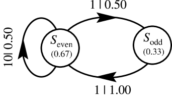
Figure 19: The recurrent portion of the $\epsilon$-machine for the even process, Example D. Since the CSs cannot be specified by a finite history of previous spins, we have labeled them ${\cal S}_{\rm even}$ and ${\cal S}_{\rm odd}$.

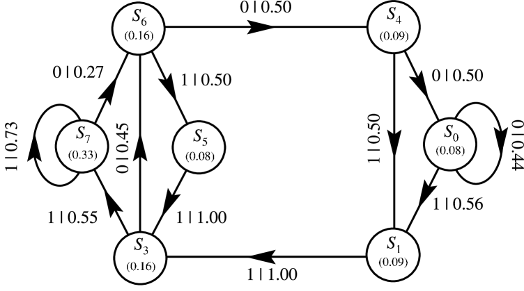
Figure 20: The ${r}=3$ reconstructed $\epsilon$-machine for the even process of Example D. Since the even process forbids the sequences $\{01^{2k+1}0,k=0,1,2,\ldots\}$ and all sequences containing them, it is satisfying to see that $010$ is forbidden by the reconstructed $\epsilon$-machine, as evidenced by the missing ${\cal S}_{2}$ CS.

We now consider a simple finite-state process that cannot be represented by a finite-order Markov process, called the even process, Crutchfield and Feldman (2003); Crutchfield (1992) as the previous examples could. The even language Hopcroft and Ullman (1979); Badii and Politi (1997) consists of sequences such that between any two $0$’s either there are no $1$s or an even number. In a sequence, therefore, if the immediately preceding spin was a $1$, then the admissibility of the next spin requires remembering the evenness of the number of previous consecutive $1$s, since seeing the last $0$. In the most general instance, this requires an indefinitely long memory and so the even process cannot be represented by any finite-order Markov chain.

We define the even process as follows: If a $0$ or an even number of consecutive $1$s were the last spin(s) seen, then the next spin is either $1$ or $0$ with equal probability; otherwise the next spin is $1$. While this might seem somewhat artificial for the stacking of simple polytypes, one cannot exclude this class of (so-called sofic) structures on physical grounds. Indeed, such long-range memories may be induced in a solid-state phase transformations between two crystal structures. Kabra and Pandey (1988b); Varn and Crutchfield It is instructive, therefore, to explore the results of our procedure on processes with such structures.

Additionally, analyzing a sofic process provides a valuable test of $\epsilon$MSR as practiced here. Specifically, we invoke a finite-order Markov approximation for the solution of the ${r}=3$ equations, and we shall determine how closely this approximates the even process with its effectively infinite range.

The $\epsilon$-machine for this process is shown in Fig. 19. Its causal-state transition structure is equivalent to that in the $\epsilon$-machine for the golden mean process. They differ only in the spins emitted upon transitions out of the ${\cal S}_{1}$ CS. It seems, then, that this process should be easy to detect.

Figure 21: A comparison of the CFs $Q_{s}(n)$ generated by the ${r}=3$ reconstructed $\epsilon$-machine and the even process of Example D. The CFs decay quickly to their asymptotic value of $1/3$.

The result of $\epsilon$-machine reconstruction at ${r}=3$ is shown in Fig. 20. Again, it is interesting to see if the sequences forbidden by the even process are also forbidden by the ${r}=3$ $\epsilon$-machine. One finds that the sequence $010$—forbidden by the process—is also forbidden by the reconstructed $\epsilon$-machine. This occurs because CS ${\cal S}_{2}$ is missing. We do notice that the reconstructed $\epsilon$-machine has much more “structure” than the original process. We now examine the source of this additional structure.

Let us first contrast differences between $\epsilon$MSR and other $\epsilon$-machine reconstruction techniques, taking the subtree-merging method (SMM) of Crutchfield and Young Crutchfield and Young (1989); Crutchfield (1994) as the alternative prototype. There are two major differences. First, since here we estimate sequence probabilities from the diffraction spectra and not a symbol sequence, we find it necessary to invoke the memory-length reduction approximation at ${r}\geq 3$ to obtain a complete set of equations. Specifically, we assume that only histories up to range ${r}$ are needed to make an optimal prediction of the next spin. Second, we assume that we can label CSs by their length-${r}$ history.

We can test these assumptions in the following way. For the first, we compare the frequencies of length-$4$ sequences obtained from each method. This is shown in Table 6. The agreement is excellent. All sequence frequencies are within $\pm 0.01$ of the correct values. The small differences are due to the memory-length reduction approximation. So this does have an effect, but it is small here.

To test the second assumption, we can compare the $\epsilon$-machines generated from each method given the same length-$4$ sequence probabilities. Doing so, SMM gives the $\epsilon$-machine for the even process shown in Fig. 19. $\epsilon$MSR gives a different result. After merging pasts with equivalent futures, one finds that shown in Fig. 22. For clarity, we explicitly show the length-$3$ sequence histories associated with each CS, but do not write out the asymptotic state probabilities.

The $\epsilon$-machine generated by $\epsilon$MSR is in some respects as good as that generated by SMM. Both reproduce the sequence probabilities up to length-$4$ from which they were estimated. The difference is that for $\epsilon$MSR, our insistence that histories be labeled by the last ${r}$-spins forces the representation to be Markovian of range ${r}$. Here, a simpler model for the process, as measured by the smaller statistical complexity ($0.92$ bits as compared to $1.92$ bits), can be found. So the notion of minimality is violated. That is, $\epsilon$MSR searches only a subset of the space from which processes can belong. Should the true process lie outside this subset (Markovian processes of range ${r}$), then $\epsilon$MSR returns an approximation to the true process. The approximation may be both more more complex and less predictive than the true process. It is interesting to note that had we given SMM the sequence probabilities found from the solutions of the spectral equations, we would have found, (within some error) the $\epsilon$-machine given in Fig. 19.

We find, then, that there are two separate consequences to applying $\epsilon$MSR that affect the reconstructed $\epsilon$-machine. The first is that for ${r}\geq 3$, the memory-length reduction approximation must be invoked to obtain a complete set of equations. This approximation limits the histories treated and can affect the values estimated for the sequence probabilities. The second is the state-labeling scheme. Only for Markovian (non-sofic) processes can CSs be labeled by a unique finite history. Making this assumption effectively limits the class of processes one can detect to those that are block-${r}$ Markovian. To see this more clearly, we can catalog the possible histories that lead to the two CSs in Fig. 19. In doing so, we find that the histories $000$, $011$, $110$, $100$, and $100$ always leave the process in CS ${\cal S}_{\rm even}$. Similarly, the histories $001$ and $101$ always leave the process in CS ${\cal S}_{\rm odd}$. But having seen the history $111$ does not specify the CS as one can arrive in both CSs from this history. So the labeling of CSs by histories fails here.

Then why do we not find sequence probabilities by solving the spectral equations and then use SMM to reconstruct the $\epsilon$-machine? There are two reasons. The first is that in general one must know sequence probabilities for longer sequences than is necessary for $\epsilon$MSR. Solving the spectral equations for these longer sequence frequencies is onerous. The second is that error in the sequence probabilities found from solving the spectral equations for these longer sequences makes identifying equivalent pasts almost impossible. The even process is an exception here, since one needs to consider only futures of length $1$. This is certainly not the case in general.

Sequence	$\epsilon$MSR	SMM	Sequence	$\epsilon$MSR	SMM
1111	0.24	0.25	0111	0.08	0.09
1110	0.09	0.08	0110	0.07	0.08
1101	0.09	0.08	0101	0.00	0.00
1100	0.08	0.08	0100	$<$ 0.01	0.00
1011	0.08	0.08	0011	0.08	0.08
1010	0.00	0.00	0010	$<$ 0.01	0.00
1001	0.04	0.04	0001	0.05	0.04
1000	0.04	0.04	0000	0.04	0.04

Table 6: The frequencies of length-$4$ sequences obtained from $\epsilon$MSR and SMM for the even process. At most, they differ by $\pm 0.01$.

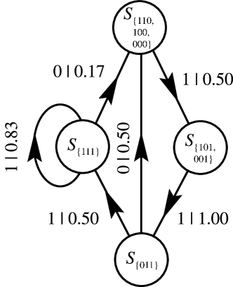
Figure 22: The $\epsilon$-machine inferred from the exact sequence frequencies. The causal states are labeled with the (possibly several) histories that can lead to them.

Having explored the differences between $\epsilon$MSR and SSM, we now return to a comparison of the results of each method. A comparison of the CFs for the even process and the reconstructed $\epsilon$-machine is given in Fig. 21. We see that both decay quite quickly to their asymptotic values of $1/3$. There is good agreement, except in the region between $5\leq n\leq 10$. Examining the diffraction spectra in Fig. 23, we see that there is likewise good agreement except in the region $0.7<l<0.9$. The profile ${\cal R}$-factor between the two spectra is ${\cal R}\approx 8\%$, which indicates that there is reasonable agreement.

There is a curious isolated zero in the process’s spectrum at $l=5/6$. The other interesting feature is the broad peak at $l\approx 1/3$. One might guess that this originates from some 3C⁺ structure and, indeed, glancing at the reconstructed $\epsilon$-machine of Fig. 20 shows that the CSC [${\cal S}_{7}$] is strongly represented. The faulting is less clear. We would expect, though, that presence of the CSC [${\cal S}_{7}{\cal S}_{6}{\cal S}_{4}{\cal S}_{0}{\cal S}_{1}{\cal S}_{3}$] would indicate layer-displacement faulting and the CSC [${\cal S}_{7}{\cal S}_{6}{\cal S}_{5}{\cal S}_{3}$] supports this.

We find by direct calculation from the even process that it has a configurational entropy of ${h_{\mu}}=0.67$ bits/spin, a statistical complexity of ${C_{\mu}}=0.92$ bits, and an excess entropy of ${\bf E}=0.91$ bits. The reconstructed $\epsilon$-machine gives information-theoretic quantities that are rather different. We find a configurational entropy ${h_{\mu}}=0.80$ bits, a statistical complexity of ${C_{\mu}}=2.63$ bits, and an excess entropy of ${\bf E}=0.22$ bits.

One reason that the reconstructed $\epsilon$-machine gives CFs and diffraction spectra in such good agreement with the even process in spite of the fact that the information-theoretic quantities are different is the insensitivity of the CFs and diffraction spectra to the probabilities of long sequences: Eq. (9) adds sequence probabilities to find CFs. The fact that the even process has such a long memory is masked by this. However, information-theoretic quantities are sensitive to the structure of long sequences. $\epsilon$-Machine reconstruction at ${r}=4$ should prove interesting, in this light, since the even process picks up another forbidden sequence—$01110$—and this additional structure would be reflected in the reconstructed $\epsilon$-machine.

Figure 23: A comparison between the diffraction spectra $\mathsf{I}(l)$ generated by the ${r}=3$ reconstructed $\epsilon$-machine and by the even process of Example D. The agreement is good except in the region $0.7<l<0.9$. Notably, the diffraction spectra for the even process has an isolated zero at $l=5/6$.

For comparison we list each of the example’s information-theoretic properties in Table 7.

System	Range	${h_{\mu}}$ [bits/ML]	${C_{\mu}}$ [bits]	${\bf E}$ [bits]	$\Delta$
Example A	3	0.44	2.27	0.95	0.00
$\epsilon$-machine	3	0.44	2.27	0.95	0.00
Example B	4	0.51	2.86	0.82	0.00
$\epsilon$-machine	3	0.54	2.44	0.83	-0.01
Example C	1	0.67	0.92	0.25	0.00
$\epsilon$-machine	1	0.67	0.92	0.25	0.00
Example D	$\infty$	0.67	0.92	0.91
$\epsilon$-machine	3	0.79	2.58	0.21	0.00

Table 7: Measures of intrinsic computation calculated from the processes of Examples A, B, C, and D and their (${r}=3$) reconstructed $\epsilon$-machines. For Examples A, B, and C the reconstructed $\epsilon$-machines give good agreement. For Example D, however, the reconstructed $\epsilon$-machine requires more memory and still has a entropy density ${h_{\mu}}$ significantly higher than that of the even process. The last column gives $\Delta={C_{\mu}}-{\bf E}-{r}{h_{\mu}}$ as a consistency check derived from Eq. (23), which describes order-${r}$ Markov processes. Recall that the even process of Example D is not a finite-${r}$ process and so Eq. (23) does not hold. All one can say is that ${\bf E}\leq{C_{\mu}}$, which is the case for Example D.

IV.5 Possible Difficulties with Applying $\epsilon$MSR

We have given four examples that demonstrate successful applications of $\epsilon$MSR. We have found instances, however, when the $\epsilon$MSR has difficulties converging to a satisfactory result. We now analyze each step in $\epsilon$MSR as given in Table 1 and discuss possible problems that may be encountered.

Step 1. Several problems can arise here. One is that the figures-of-merit, $\beta$ and $\gamma$, are sufficiently different from their theoretical values over all possible $l$-intervals that $\epsilon$MSR should not even be attempted. Even if one does find an interval such that they indicate satisfactory spectral data, it is possible that the CFs extracted over this interval are unphysical. That is, there is no guarantee that all of the CFs are both positive and less than unity. In such a case, no stacking of MLs can reproduce these CFs. Finally, if error ranges have not been reported with the experimental data, it may not be possible to set the error threshold $\Gamma$.

Step 2. The ${\rm P}(\omega^{r})$ solutions to the spectral equations are not guaranteed to be either real or positive for ${r}\geq 3$. If this is so, then no physical stacking of MLs can reproduce the CFs from the spectrum.

Step 3. Given ${\rm P}(\omega^{r})$ that satisfy the elementary conditions of probability (i.e., there is no difficulty at step 2), step 3 will return a machine that generates ${\rm P}(\omega^{r})$. It is possible, however, that the resulting states are not strongly connected, and thus the result may not be interpreted as a single $\epsilon$-machine.

Step 4. There are no difficulties here.

Step 5. It is possible that one is required to go to an ${r}$ that is cumbersome to calculate. In this case, one terminates the procedure through practicality.

We find that the roots of these difficulties can be ultimately traced to four problems: (i) excessive error in the diffraction spectrum, (ii) the process has statistics that are too complex to be captured by a finite-range Markov process, (iii) the memory-length approximation is not satisfied, and (iv) the initial assumptions of polytypism are violated. We are likely to discover (i) in step 1. For (ii) and (iii), we find no difficulties at step 1, but rather at steps 2, 3, and 5. For (iv), we have not examined this case in detail. However, we expect that if the assumptions of the stacking of MLs (§III) are not met, then since Eq. (1) is no longer valid, the CFs found by Fourier analysis will not reflect the actual stacking probabilities. This will likely be interpreted as poor figures-of-merit, and $\epsilon$MSR will terminate at step 1.

Of the three possible difficulties only (ii) and (iii) should be considered to be inherent to $\epsilon$MSR. It is satisfying that $\epsilon$MSR can detect errors in the diffraction spectrum and then stop, so that it does not generate an invalid representation that simply describes “error” or “noise”.

V Characteristic Lengths in CPSs

We now return to one of the mysteries of polytypism, namely that of the long-range order which they seem to possess. It is of interest, then, to ask what, if anything, the spectrally reconstructed $\epsilon$-machine indicates about the range of interactions between MLs. In this section, we discuss and quantify several characteristic lengths that can be estimated from reconstructed $\epsilon$-machines.

(i) Correlation Length, $\lambda_{c}$. From statistical mechanics, we have the notion of a correlation length, Binney et al. (1993); Yeomans (1992) which is simply the characteristic length scale over which “structures” are found. The correlation functions $Q_{c}(n)$, $Q_{a}(n)$, and $Q_{s}(n)$ are known to decay to $1/3$ for many disordered stackings. (For some exceptions, see Kabra and Pandey, Kabra and Pandey (1988b) Yi and Canright, Yi and Canright (1996) and Varn. Varn (2001)) For the disordered cases considered here, exponential decay to $1/3$ seems to be the rule. We therefore define the correlation length $\lambda_{c}$ as the characteristic length over which correlation information is lost with increasing separation $n$. More precisely, let us define $\Psi_{q}(n)$ as

$$\Psi_{q}(n)=\sum_{\alpha}\Bigl{|}Q_{\alpha}(n)-\frac{1}{3}\Bigr{|}~{},$$ (28)

so that $\Psi_{q}(n)$ gives a measure of the deviation of the CFs from their asymptotic value. Then we say that

$$\Psi_{q}(n)=F(n)\times 2^{-n/\lambda_{c}}~{},$$ (29)

where $F(n)$ is some function of $n$.

For those cases where the CFs do not decay to $1/3$, we say that the correlation length is infinite. We find that exponential decay is not always obeyed, but it seems to be common,not (f) and the correlation length thus defined gives a useful measure of the rate of coherence loss as $n$ increases. Our definition of correlation length is similar to the characteristic length $L$ defined by Shrestha and Pandey. Shrestha and Pandey (1996a, 1997)

(ii) Recurrence Length, $\mathcal{P}$. For an exactly periodic process, the period gives the length over which a template pattern repeats itself. We can generalize this for arbitrary, aperiodic processes in the following way. Let us take the recurrence length $\mathcal{P}$ as the geometric mean of the distances between visits to each CS weighted by the probability to visit that CS:

$$\mathcal{P}\equiv\prod_{{\cal S}_{i}\in{\cal S}}T_{i}^{p_{i}}~{},$$ (30)

where $T_{i}$ is the average distance between visits to a CS and $p_{i}$ is the probability of visiting that CS. Then,

$$\mathcal{P} = \prod_{{\cal S}_{i}\in{\cal S}}(2^{\log_{2}T_{i}})^{p_{i}}$$ (31)

$$= \prod_{{\cal S}_{i}\in{\cal S}}2^{-p_{i}\log_{2}p_{i}}$$

$$= 2^{-\sum_{{\cal S}_{i}\in{\cal S}}p_{i}\log_{2}p_{i}}$$

$$= 2^{{C_{\mu}}}~{},$$

where we have used the relation $T_{i}=1/p_{i}$.

For periodic processes, ${C_{\mu}}=\log_{2}\mathcal{P}$ and so $\mathcal{P}$ is simply a process’s period. For aperiodic processes $\mathcal{P}$ gives a measure of the average distance over which the $\epsilon$-machine returns to a CS. Notice that this is defined as the average recurrence length in the Hägg notation. For cubic and rhombohedral structures, for example, this is one-third of the physical repeat distance in the absolute stacking sequence.

(iii) Memory Length, ${r}_{l}$. Recall from §II.7 that the memory length is an integer which specifies the maximum number of previous spins that one must know in the worst case to make an optimal prediction of the next spin. For an ${r}^{\mathrm{th}}$-order Markov process this is ${r}$.

(iv) Interaction Length, ${r}_{I}$. The interaction length is an integer that gives the maximum range over which spin-spin interactions appear in the Hamiltonian.

We calculated the $\lambda_{c}$, $\mathcal{P}$, and ${r}_{l}$ (in units of MLs) for Examples A-D as well as for three crystal structures. The results are displayed in Table 8. We see that each captures a different aspect of the system. The correlation length $\lambda_{c}$ sets a scale over which a process is coherent. For crystals, as shown in Table 8, this length is infinite. For more disordered systems, this value decreases. The generalized period $\mathcal{P}$ is a measure of the scale over which the pattern produced by the process repeats. The memory length ${r}_{l}$ is most closely related to what we might think as the maximum range of “influence” of a spin. That is, it is the maximum distance over which one might need to look to obtain information to predict a spin’s value.

For periodic, infinitely correlated systems spins at large separation carry information about each other, as seen in crystals. But this information is redundant. Outside a small neighborhood one gets no additional information by knowing the orientation a spin assumes. Notice that one can have an infinite memory length with a relatively small correlation length, as seen for the even system (Example D). That is, even though on average the knowledge one has about a spin may decay, there are still configurations in which distantly separated spins carry information about each other that is not stored in the intervening spins.

If we know the $\epsilon$-machine for a process, then we can directly calculate $\lambda_{c}$, $\mathcal{P}$, and ${r}_{l}$. How, then, do these relate to the interaction length ${r}_{I}$? Infinite correlation lengths can be achieved with very small ${r}_{I}$, as in the case of simple crystals. So correlation lengths alone imply little about the range of interactions. For a periodic system in the ground state, the configuration’s period puts a lower bound on the interaction length via ${r}_{I}\geq\log_{2}\mathcal{P}$—barring fine tuning of parameters, such as found at the multiphase boundaries in the ANNNI model Yeomans (1988) or those imposed by symmetry considerations. Varn and Canright (2001); Canright and Watson (1996) This does not hold, however, for systems above the ground state. The most likely candidate for a useful relation between ${r}_{I}$ and a quantity generated from the $\epsilon$-machine is ${r}_{l}$. Again, ${r}_{l}$ sets a lower bound on ${r}_{I}$, if the system is in the ground state. For polytypes, the multitude of observed structures suggests that most are not in the ground state and, thus, one does not know what the relation between ${r}_{I}$ and ${r}_{l}$ is. It is conceivable, especially in the midst of a solid-state phase transition, that small ${r}_{I}$ could generate large ${r}_{l}$. Although, an $\epsilon$-machine is a complete description of the underlying stacking process, one should be able to calculate from it the interaction length in the case that the system not in the ground state. We suspect the answer lies in the different ways in which a Hamiltonian and an $\epsilon$-machine describe a material.

System	$\lambda_{c}$	$\mathcal{P}$	${r}_{l}$
Example A, ${r}=3$	$\sim 7.4$	4.8	3
Example B, ${r}=4$	$\sim 7.8$	7.3	4
Example C, Golden Mean	$\sim 4.5$	1.9	$1$
Example D, Even Process	$\sim 1.7$	1.9	$\infty$
3C	$\infty$	1	0
2H	$\infty$	2	1
6H	$\infty$	6	3

Table 8: A comparison of the three characteristic lengths that one can calculate from knowledge of the $\epsilon$-machine: the correlation length $\lambda_{c}$, the recurrence length $\cal P$, and the memory length ${r}_{l}$.

VI Conclusions

We offer here a new way of treating planar disorder in CPSs. We find the minimal, unique description of the stacking for any amount and kind of ordered and disordered sequence that a material may contain. We demonstrated how this description—the $\epsilon$-machine—can be directly inferred from experimental diffraction spectra. $\epsilon$MSR uses all of the information in the spectrum, both Bragg-like and diffuse scattering. Our description is necessarily statistical, in that we do not find the specific stacking sequence that gave rise to the diffraction pattern, but rather a minimal description of the ensemble of stackings that could have generated the diffraction spectrum. We contend that this statistical description is the most useful form in which to express the structure of the crystal. From it, physical parameters such as the entropy per ML, the statistical complexity, and the average stacking-fault energy for disordered stacking sequences are calculable. Varn et al. (2002b) Indeed, could we have found a specific stacking sequence millions of MLs in length, one still would search for some way to compress this information into a useful form. In short, one would want to find its $\epsilon$-machine. We therefore state that our solution—which is directly determined from experimental diffraction spectra—offers the most complete and compact understanding of the stacking process and, thus, of the solid’s structure. On this basis, we say that (i) $\epsilon$MSR has solved the problem of inferring structural information from diffraction spectra for CPSs and (ii) the resulting $\epsilon$-machine is the unique and minimal expression of that structure.

We illustrated the approach by solving the inference problem for ${r}=3$, which gives stacking-sequence probabilities up to length $4$. Unlike previous work, we considered all the possible sequences of this length without invoking symmetry arguments. This highlights the need for good experimental data. It is important to get accurate diffraction spectra over a unit $l$-interval that records the intensity of both the Bragg-like peaks and the diffuse scattering. We have shown that there exist quantities, called the figures-of-merit, that measure the quality of the spectral data over a particular unit $l$-interval and that help determine a suitable interval for $\epsilon$-machine spectral reconstruction.

While we have addressed only CPSs here, the extension to other layered structures is straightforward. A first theoretical task in this is to find an expression for the diffracted intensity in terms of suitable CFs and to relate these CFs to the sequence distribution (and thence to an $\epsilon$-machine). While such an $\epsilon$-machine may draw from an alphabet larger than two for more complicated polytypes, such as micas and kaolins, Varn and Canright (2001) there are in principle no theoretical obstacles to applying $\epsilon$MSR to more complicated polytypic structures.

More generally, $\epsilon$MSR also contributes to the machine-learning side of computational mechanics. $\epsilon$MSR is novel, in that we use a power spectrum to reconstruct the $\epsilon$-machine instead of a temporal data sequence, as prior algorithms have. We see this as a prelude to the question of how one infers an $\epsilon$-machine from general spectral data and are continuing research along these lines.

There are, however, some limitations to $\epsilon$MSR, as presented here. We only attempted $\epsilon$-machine reconstruction up to ${r}=3$. While in principle one can attempt it for any ${r}$, there are computational complexity difficulties. In the most general case, the number of variables one needs to solve for is exponential in ${r}$, and many of the equations are nonlinear. More seriously, the maximum number of terms in any equation grows as an exponential of an exponential in ${r}$. For ${r}=3$, there were $11$ terms in two of the equations. At ${r}=4$, two of the equations have $171$ terms, all of them nonlinear. For ${r}=5$, this grows to $43690$ terms. Varn (2001) These terms are all additive, so a fortuitous cancellation is not possible. It is possible, however, that physical insight into the relative importance of sequences may allow one to neglect a number of terms in these equations. We feel that the general case of ${r}=4$ is tractable, and this is a subject of current research. We also suspect that there are alternative algorithms that will greatly reduce the computational complexity of finding solutions.

Finally, we stress that there is a difference between structure and mechanism in disordered stacking sequences. The $\epsilon$-machine describes the structure, but has little to say about how the material came to be stacked in this fashion. While it is possible to formally identify CSCs with “faulting structures”, this can be misleading. It is certainly possible that the cumulative effects of repeated faulting by a particular mechanism may lead to a structure that is different from a crystal simply permeated with that kind of fault. That is, for high fault densities, adjacent faults may be produced in the same way, but the close proximity of the faults may cause us to interpret the structure differently—e.g., as a small segment of complex crystal.

In order to determine the mechanism of faulting in, say, an annealed crystal undergoing a solid-state phase transition, it is desirable to begin with many (identical) crystals and arrest the solid-state transformation at various stages. By reconstructing the $\epsilon$-machine after different annealing times, the route to disorder can be made plain. The result is a picture of how structure (as captured by intermediate $\epsilon$-machines) changes during annealing. This change in structure should give direct insight into the structure-forming mechanisms. This should be compared with the numerical simulation of faulting in a crystal, such as those done by Kabra and Pandey, Kabra and Pandey (1988b) Engel, Engel (1990) Shrestha and Pandey, Shrestha and Pandey (1996a, 1997) Gosk, Gosk (2000, 2001) and Ramasesha and Rao. Ramasesha and Rao (1977) We note that in such simulations, the $\epsilon$-machine can be directly calculated from the sequence to high accuracy. Some experimental work on solid-state phase transitions has been done, Sebastian and Krishna (1994) but we hope that there will be additional effort in this direction.

Appendix A The Spectral Equations

A.1 ${r}=1$

The spectral equations at ${r}=1$ are linear and admit an analytical solution. Specifically, we write out Eqs. (7), (8), and (9) for ${r}=1$ and solve them. We find,

$${\rm P}(11) = Q_{r}(2)~{},$$

$${\rm P}(01) = p(10)=\frac{1}{2}[1-Q_{c}(2)-Q_{r}(2)]~{},$$

$${\rm P}(00) = Q_{c}(2)~{}.$$

A.2 ${r}=2$

Similarly, the spectral equations at ${r}=2$ are linear and also can be solved analytically. Again, we write out Eqs. (7), (8), and (9) for ${r}=2$ and solve them. We find,

$${\rm P}(000) = [3Q_{c}(2)-2Q_{c}(3)-3Q_{r}(2)-4Q_{r}(3)+3]/6~{},$$

$${\rm P}(001) = [3Q_{c}(2)+2Q_{c}(3)+3Q_{r}(2)+4Q_{r}(3)-3]/6~{},$$

$${\rm P}(010) = [-3Q_{c}(2)-2Q_{c}(3)-3Q_{r}(2)-Q_{r}(3)+3]/3~{},$$

$${\rm P}(011) = [3Q_{c}(2)+4Q_{c}(3)+3Q_{r}(2)+2Q_{r}(3)-3]/6~{},$$

$${\rm P}(100) = [3Q_{c}(2)+2Q_{c}(3)+3Q_{r}(2)+4Q_{r}(3)-3]/6~{},$$

$${\rm P}(101) = [-3Q_{c}(2)-Q_{c}(3)-3Q_{r}(2)-2Q_{r}(3)+3]/3~{},$$

$${\rm P}(110) = [3Q_{c}(2)+4Q_{c}(3)+3Q_{r}(2)+2Q_{r}(3)-3]/6~{},$$

$${\rm P}(111) = [-3Q_{c}(2)-4Q_{c}(3)+3Q_{r}(2)-2Q_{r}(3)+3]/6~{}.$$

A.3 ${r}=3$

At ${r}=3$, we require $16$ relations to constrain the length-$4$ binary-sequence probabilities. Now, however, we encounter nonlinearities, and by necessity the spectral equations are solved numerically. We write them out here.

At ${r}=3$, Eq. (7) implies the following seven equations.

$${\rm P}(0111) = {\rm P}(1110)~{},$$

$${\rm P}(0001) = {\rm P}(1000)~{},$$

$${\rm P}(0011)+{\rm P}(1011) = {\rm P}(0111)+{\rm P}(0110)~{},$$

$${\rm P}(0101)+{\rm P}(1101) = {\rm P}(1011)+{\rm P}(1010)~{},$$

$${\rm P}(0010)+{\rm P}(1010) = {\rm P}(0101)+{\rm P}(0100)~{},$$

$${\rm P}(0001)+{\rm P}(1001) = {\rm P}(0011)+{\rm P}(0010)~{},$$

$${\rm P}(0100)+{\rm P}(1100) = {\rm P}(1001)+{\rm P}(1000)~{}.$$

Equation (8) provides for normalization, providing one additional constraint. Finally, the remaining $8$ relations are obtained by relating sequence probabilities to CFs as prescribed by Eq. (9). We further reduce the last two relations which involve sequence probabilities of length-$5$ to those of length-$4$ via relations of the form given by Eq. (10). We find,

$$Q_{c}(2) = {\rm P}(0000)+{\rm P}(0001)+{\rm P}(0010)+{\rm P}(0011)~{},$$

$$Q_{r}(2) = {\rm P}(1100)+{\rm P}(1101)+{\rm P}(1110)+{\rm P}(1111)~{},$$

$$Q_{c}(3) = {\rm P}(0110)+{\rm P}(0111)+{\rm P}(1010)+{\rm P}(1011)$$

$$+{\rm P}(1100)+{\rm P}(1101)~{},$$

$$Q_{r}(3) = {\rm P}(0010)+{\rm P}(0011)+{\rm P}(0100)+{\rm P}(0101)$$

$$+{\rm P}(1000)+{\rm P}(1001)~{},$$

$$Q_{c}(4) = {\rm P}(1111)+{\rm P}(1000)+{\rm P}(0100)+{\rm P}(0010)$$

$$+{\rm P}(0001)~{},$$

$$Q_{r}(4) = {\rm P}(0000)+{\rm P}(0111)+{\rm P}(1011)+{\rm P}(1101)$$

$$+{\rm P}(1110)~{},$$

$$Q_{c}(5) = \frac{{\rm P}^{2}(0000)}{{\rm P}(0000)+{\rm P}(0001)}+\frac{{\rm P}(0011){\rm P}(0111)}{{\rm P}(0111)+{\rm P}(0110)}$$

$$+\frac{{\rm P}(0101){\rm P}(1011)}{{\rm P}(1011)+{\rm P}(1010)}+\frac{{\rm P}(0110){\rm P}(1101)}{{\rm P}(1101)+{\rm P}(1100)}$$

$$+\frac{{\rm P}(0111){\rm P}(1110)}{{\rm P}(1110)+{\rm P}(1111)}+\frac{{\rm P}(1001){\rm P}(0011)}{{\rm P}(0011)+{\rm P}(0010)}$$

$$+\frac{{\rm P}(1010){\rm P}(0101)}{{\rm P}(0101)+{\rm P}(0100)}+\frac{{\rm P}(1011){\rm P}(0110)}{{\rm P}(0110)+{\rm P}(0111)}$$

$$+\frac{{\rm P}(1100){\rm P}(1001)}{{\rm P}(1001)+{\rm P}(1000)}+\frac{{\rm P}(1101){\rm P}(1010)}{{\rm P}(1010)+{\rm P}(1011)}$$

$$+\frac{{\rm P}(1110){\rm P}(1100)}{{\rm P}(1100)+{\rm P}(1101)}~{},$$

$$Q_{r}(5) = \frac{{\rm P}^{2}(1111)}{{\rm P}(1111)+{\rm P}(1110)}+\frac{{\rm P}(1100){\rm P}(1000)}{{\rm P}(1000)+{\rm P}(1001)}$$

$$+\frac{{\rm P}(1010){\rm P}(0100)}{{\rm P}(0100)+{\rm P}(0101)}+\frac{{\rm P}(1001){\rm P}(0010)}{{\rm P}(0010)+{\rm P}(0011)}$$

$$+\frac{{\rm P}(1000){\rm P}(0001)}{{\rm P}(0001)+{\rm P}(0000)}+\frac{{\rm P}(0110){\rm P}(1100)}{{\rm P}(1100)+{\rm P}(1101)}$$

$$+\frac{{\rm P}(0101){\rm P}(1010)}{{\rm P}(1010)+{\rm P}(1011)}+\frac{{\rm P}(0100){\rm P}(1001)}{{\rm P}(1001)+{\rm P}(1000)}$$

$$+\frac{{\rm P}(0011){\rm P}(0110)}{{\rm P}(0110)+{\rm P}(0111)}+\frac{{\rm P}(0010){\rm P}(0101)}{{\rm P}(0101)+{\rm P}(0100)}$$

$$+\frac{{\rm P}(0001){\rm P}(0011)}{{\rm P}(0011)+{\rm P}(0010)}~{}.$$

References

- von Laue (1918) M. von Laue, Ann. Phys., Lpz. 56, 497 (1918).
- Frey (1995) F. Frey, Acta Crystallogr., Sec. B 51, 592 (1995).
- Jagodzinski (1987) H. Jagodzinski, Progress in Crystal Growth and Characterization of Materials 14, 47 (1987).
- Proffen and Welberry (1998) T. Proffen and T. R. Welberry, Phase Transitions 67, 373 (1998).
- Welberry (1985) T. R. Welberry, Rep. Prog. Phys. 48, 1543 (1985).
- Schulz (1982) H. Schulz, in Current Topics in Materials Science, edited by E. Kaldis (North-Holland, Amsterdam, 1982), vol. 8.
- Guinier (1963) A. Guinier, X-Ray Diffraction in Crystals, Imperfect Crystals, and Amorphous Bodies (W.H. Freeman and Company, 1963).
- Woolfson (1997) M. M. Woolfson, An Introduction to X-ray Crystallography (Cambridge, 1997).
- Hirth and Lothe (1982) J. P. Hirth and J. Lothe, Theory of Dislocations (John Wiley, 1982), 2nd ed.
- Ashcroft and Mermin (1976) N. W. Ashcroft and N. D. Mermin, Solid State Physics (Saunders College Publishing, 1976).
- Kittel (1996) C. Kittel, Introduction to Solid State Physics (John Wiley & Sons, 1996), 7th ed.
- Sebastian and Krishna (1994) M. T. Sebastian and P. Krishna, Random, Non-Random and Periodic Faulting in Crystals (Gordon and Breach, 1994).
- Frank (1951a) F. C. Frank, Philos. Mag. 42, 809 (1951a).
- Frey and Boysen (1981) F. Frey and H. Boysen, Acta Crystallogr., Sec. A 37, 819 (1981).
- Verma and Krisha (1966) A. R. Verma and P. Krisha, Polymorphism and Polytypism in Crystals (John Wiley & Sons, 1966).
- Trigunayat (1991) G. C. Trigunayat, Solid State Ionics 48, 3 (1991).
- Pandey and Krishna (1982) D. Pandey and P. Krishna, in Current Topics in Materials Science, edited by E. Kaldis (North-Holland, 1982).
- Frevel et al. (1992) L. K. Frevel, D. R. Petersen, and C. K. Saha, J. Mater. Sci. 27, 1913 (1992).
- Baumhauer (1912) H. Baumhauer, Z. Kristallogr. 50, 33 (1912).
- not (a) This is only approximately true. For a recent discussion, see G. C. Trigunayat, Solid State Ionics 48, 3 (1991).
- Varn and Canright (2001) D. P. Varn and G. S. Canright, Acta Crystallogr. Sec. A 57, 4 (2001).
- Engel and Needs (1990) G. E. Engel and R. J. Needs, J. Phys. Cond. Mat. 2, 367 (1990).
- Cheng et al. (1987) C. Cheng, R. J. Needs, V. Heine, and N. Churcher, Europhys. Lett. 4, 475 (1987).
- Shaw and Heine (1990) J. J. A. Shaw and V. Heine, J. Phys. Cond. Mat. 2, 4351 (1990).
- Frank (1951b) F. C. Frank, Philos. Mag. 42, 1014 (1951b).
- Jagodzinski (1954) H. Jagodzinski, Acta Crystallogr. 7, 300 (1954).
- Yeomans (1988) J. Yeomans, Solid State Physics 41, 151 (1988).
- Pandey (1989) D. Pandey, Phase Transitions 16/17, 247 (1989).
- Landau (1937) L. Landau, Phys. Z. Sowjetunion 12, 579 (1937).
- Lifschitz (1937) I. M. Lifschitz, Phys. Z. Sowjetunion 12, 623 (1937).
- Wilson (1942) A. J. C. Wilson, Proc. R. Soc. Ser. A 180, 277 (1942).
- Hendricks and Teller (1942) S. Hendricks and E. Teller, J. Chem. Phys. 10, 147 (1942).
- Jagodzinski (1949a) H. Jagodzinski, Acta Crystallogr. 2, 201 (1949a).
- Jagodzinski (1949b) H. Jagodzinski, Acta Crystallogr. 2, 208 (1949b).
- Barrett (1950) C. S. Barrett, Trans. Metall. Soc. AIME 188, 123 (1950).
- Patterson (1952) M. S. Patterson, J. Appl. Phys. 23, 805 (1952).
- not (b) For close-packed crystal structures it is common to use the Ramsdell notation, nX, where n gives the total number of ML’s in the unit cell and X specifies the crystal symmetry. We use H to denote hexagonal symmetry, C for cubic, R for rhombohedral and L if the symmetry is unknown. This notation is not necessarily unique for some longer period polytypes. We will use the Ramsdell notation to specify crystal structures. The equivalents in the Hägg notation are given in Table 2. For a more complete discussion, see Ref. Sebastian and Krishna, 1994.
- Gevers (1954a) R. Gevers, Acta Crystallogr. 7, 492 (1954a).
- Gevers (1954b) R. Gevers, Acta Crystallogr. 7, 337 (1954b).
- Johnson (1963) C. A. Johnson, Acta Crystallogr. 16, 490 (1963).
- Prasad and Lele (1970) B. Prasad and S. Lele, Acta Crystallogr., Sec. A 26, 54 (1970).
- Pandey and Krishna (1976) D. Pandey and P. Krishna, Acta Crystallogr., Sec. A 32, 488 (1976).
- Pandey and Krishna (1977) D. Pandey and P. Krishna, J. Phys. D. 10, 2057 (1977).
- Michalski (1988) E. Michalski, Acta Crystallogr. A 44, 640 (1988).
- Michalski et al. (1988) E. Michalski, S. Kaczmarek, and M. Demianiuk, Acta Crystallogr. A 44, 650 (1988).
- Pandey et al. (1980a) D. Pandey, S. Lele, and P. Krishna, Proc. R. Soc. London Ser. A 369, 435 (1980a).
- Pandey et al. (1980b) D. Pandey, S. Lele, and P. Krishna, Proc. R. Soc. London Ser. A 369, 451 (1980b).
- Pandey et al. (1980c) D. Pandey, S. Lele, and P. Krishna, Proc. R. Soc. London Ser. A 369, 463 (1980c).
- Sebastian (1988) M. T. Sebastian, J. Mat. Sci. 23, 2014 (1988).
- Sebastian and Krishna (1984) M. T. Sebastian and P. Krishna, Philos. Mag. A 49, 809 (1984).
- Sebastian and Krishna (1987a) M. T. Sebastian and P. Krishna, Crys. Res. Tech. 22, 929 (1987a).
- Sebastian and Krishna (1987b) M. T. Sebastian and P. Krishna, Crys. Res. Tech 22, 1063 (1987b).
- Sebastian et al. (1982) M. T. Sebastian, D. Pandey, and P. Krishna, Phys. Status Solidi A 71, 633 (1982).
- Frey et al. (1986) F. Frey, H. Jagodzinski, and G. Steger, Bull. Min. 109, 117 (1986).
- Pandey and Lele (1986a) D. Pandey and S. Lele, Acta Metall. 34, 405 (1986a).
- Pandey and Lele (1986b) D. Pandey and S. Lele, Acta Metall. 34, 415 (1986b).
- Jagodinski (1972) H. Jagodinski, Sov. Phys. Crystallogr. 16, 1081 (1972).
- (58) D. P. Varn, J. P. Crutchfield, and G. S. Canright, unpublished.
- Dornberger-Schiff (1972) K. Dornberger-Schiff, Sov. Phys. Crystallogr. 16, 1091 (1972).
- Farkas-Jahnke (1973a) M. Farkas-Jahnke, Acta Crystallogr., Sec. B 29, 407 (1973a).
- Farkas-Jahnke (1973b) M. Farkas-Jahnke, Acta Crystallogr., Sec. B 29, 413 (1973b).
- Gosk (2000) J. B. Gosk, Crys. Res. Tech. 35, 101 (2000).
- Palosz and Przedmojski (1976) B. Palosz and J. Przedmojski, Acta Crystallogr., Sec. A 32, 409 (1976).
- Treacy et al. (1991) M. M. J. Treacy, J. M. Newsam, and M. W. Deem, Proc. R. Soc. London, Ser. A 433, 499 (1991).
- Kabra and Pandey (1988a) V. K. Kabra and D. Pandey, Act Crystallogr. Sec. A 51, 329 (1988a).
- Krishna and Marshall (1971a) P. Krishna and R. C. Marshall, J. Cryst. Growth 11, 147 (1971a).
- Krishna and Marshall (1971b) P. Krishna and R. C. Marshall, J. Cryst. Growth 9, 319 (1971b).
- Sebastian and Krishna (1987c) M. T. Sebastian and P. Krishna, Phys. Stat. Sol. A 101, 329 (1987c).
- Sebastian et al. (1987) M. T. Sebastian, K. Narayanan, and P. Krishna, Phys. Stat. Sol. A 102, 241 (1987).
- Shrestha and Pandey (1996a) S. P. Shrestha and D. Pandey, Europhys. Lett. A 34, 269 (1996a).
- Shrestha and Pandey (1996b) S. P. Shrestha and D. Pandey, Acta Mater. 44, 4949 (1996b).
- Shrestha et al. (1996) S. P. Shrestha, V. Tripathi, V. K. Kabra, and D. Pandey, Acta Mater. 44, 4937 (1996).
- Shrestha and Pandey (1997) S. P. Shrestha and D. Pandey, Proc. R. Soc. London Ser. A 453, 1311 (1997).
- not (c) There are other techniques for discovering structure in solids that do use the diffuse scattering quantitatively, such as reverse Monte Carlo simulation [D. A. Keen and R. L. McGreevy, Nature 344, 423 (1990)], but to our knowledge these have not been applied to planar disorder in CPS’s.
- Varn et al. (2002a) D. P. Varn, G. S. Canright, and J. P. Crutchfield, Phys. Rev. B. 66, 156 (2002a).
- Crutchfield and Young (1989) J. P. Crutchfield and K. Young, Phys. Rev. Lett. 63, 105 (1989).
- Crutchfield and Feldman (1997) J. P. Crutchfield and D. P. Feldman, Phys. Rev. E 55, R1239 (1997).
- Crutchfield and Feldman (2003) J. P. Crutchfield and D. P. Feldman, CHAOS (2003), in press.
- Feldman and Crutchfield (1998) D. P. Feldman and J. P. Crutchfield, Santa Fe Institute Working Paper 98-04-026 (1998).
- Shalizi and Crutchfield (2001) C. R. Shalizi and J. P. Crutchfield, J. Stat. Phys. 104, 819 (2001).
- Feldman (1998) D. P. Feldman, Ph.D. thesis, University of California, Davis (1998).
- Varn et al. (2002b) D. P. Varn, G. S. Canright, and J. P. Crutchfield, unpublished (2002b).
- Hansen (1993) J. E. Hansen, Ph.D. thesis, University of California, Berkeley (1993).
- Crutchfield and Young (1990) J. P. Crutchfield and K. Young, in Complexity, Entropy, and the Physics of Information, edited by W. H. Zurek (Addison-Wesley, 1990), vol. VIII of Santa Fe Institute Studies in the Sciences of Complexity.
- Gonçalves et al. (1998) W. M. Gonçalves, R. D. Pinto, J. C. Sartorelli, and M. J. de Oliveira, Physica A 257, 385 (1998).
- Palmer et al. (2000) A. J. Palmer, C. W. Fairall, and W. A. Brewer, IEEE Trans. Geosci. Remote Sens. 38, 2056 (2000).
- Clarke et al. (2001) R. W. Clarke, M. P. Freeman, and N. W. Watkins, cond-mat/0110228 (2001).
- Crutchfield (1994) J. P. Crutchfield, Physica D 75, 11 (1994).
- Shalizi et al. (2002) C. R. Shalizi, K. L. Shalizi, and J. P. Crutchfield, Santa Fe Institute Working Paper 02-10-060 (2002).
- Yi and Canright (1996) J. Yi and G. S. Canright, Phys. Rev. B 53, 5198 (1996).
- not (d) We use the standard notation here, with being the Miller indices corresponding to the -ML hexagonal cell with the stacking direction chosen along the [00.1] direction. We set and as is typically reported from experiment. The stacking direction is perpendicular to the faulted planes in the cubic lattice {111}. Note that our definition of (see text) differs from that of many authors.Sebastian and Krishna (1994) See A. Guinier, X-Ray Diffraction in Crystals, Imperfect Crystals and Amorphous Bodies (W. H. Freeman and Company, 1963) and references therein for a discussion of typical geometries and notations.
- Berliner and Werner (1986) R. Berliner and S. Werner, Phys. Rev. B 34, 3586 (1986).
- Hahn et al. (1992) T. Hahn, A. J. C. Wilson, and U. Shmueli, eds., International Tables for Crystallography, , revised edition (Kluwer Academic publishers, 1992).
- Milburn (1973) G. H. W. Milburn, X-ray Crystallography: An Introduction to the Theory and Practice of Single-crystal Structure Analysis (Butterworth & Company, 1973).
- Varn (2001) D. P. Varn, Ph.D. thesis, University of Tennessee, Knoxville (2001).
- not (e) Our definition of the profile -factor differs somewhat from that used by other authors.Berliner and Werner (1986) We perform an integral over a unit -interval instead of summing the magnitude of the difference between theory and experiment. Also, we find it convenient to compare the corrected diffraction intensities , rather than the total diffracted intensity as is done elsewhere. Our definition remains true to the spirit of the original, however.
- Pandey et al. (1987) D. Pandey, L. Prasad, S. Lele, and J. P. Gauthier, J. Appl. Crystallogr. 34, 415 (1987).
- Teubner (1990) M. Teubner, Physica A 169, 407 (1990).
- Canright and Watson (1996) G. S. Canright and G. Watson, J. Stat. Phys. 84, 1095 (1996).
- Crutchfield (1992) J. P. Crutchfield, in Santa Fe Studies in the Sciences of Complexity, edited by M. Casdagli and S. Eubanks (Addison-Wesley, Reading, Massachusetts, 1992), vol. XII.
- Hopcroft and Ullman (1979) J. E. Hopcroft and J. D. Ullman, Introduction to Automata Theory, Languages, and Computation (Addison-Wesley, 1979).
- Badii and Politi (1997) R. Badii and A. Politi, Complexity: Hierarchical Structures and Scaling and Physics, vol. 6 of Cambridge Nonlinear Science Series (Cambridge University Press, 1997).
- Kabra and Pandey (1988b) V. K. Kabra and D. Pandey, Phys. Rev. Lett. 61, 1493 (1988b).
- (104) D. P. Varn and J. P. Crutchfield, unpublished.
- Binney et al. (1993) J. J. Binney, N. J. Dowrick, A. J. Fisher, and M. E. J. Newman, The Theory of Critical Phenomena (Clarendon Press, 1993).
- Yeomans (1992) J. Yeomans, Statistical Mechanics of Phase Transitions (Clarendon Press, 1992).
- not (f) Crutchfield and FeldmanCrutchfield and Feldman (2003) discuss the exponential decay of correlations.
- Engel (1990) G. E. Engel, J. Phys. Cond. Mat. 2, 6905 (1990).
- Gosk (2001) J. B. Gosk, Crys. Res. Tech. 36, 197 (2001).
- Ramasesha and Rao (1977) S. Ramasesha and C. N. O. Rao, Philos. Mag. 36, 827 (1977).