Granular clustering in a hydrodynamic simulation

Abstract

We examine the hydrodynamics of a granular gas using numerical simulation. We demonstrate the appearance of shearing and clustering instabilities predicted by linear stability analysis, and show that their appearance is directly related to the inelasticity of collisions in the material. We discuss the rate at which these instabilities arise and the manner in which clusters grow and merge.

One of the key differences between a granular material and a regular fluid is that the grains of the former lose energy with each collision, while the molecules of the latter do not. Even when the inelasticity of the collisions is small, it can give rise to dramatic effects, such as the Maxwell Demon effecteggers and, the topic of this paper, the phenomenon of granular clustering. Experimentskudrolli ; olafsen and molecular dynamics simulationsgoldhirsch alike show that low-density collections of grains (“granular gases”) in the absence of gravity do not become homogeneous with time, but instead form denser clusters of stationary particles surrounded by a lower density region of more energetic particles. A kinetic explanation for this behavior is that, when a particle enters a region of slightly higher density, it has more collisions, loses more energy, and so is less able to leave that region. This increases the local density and makes it more likely that additional particles are captured in the same way.

We are interested in describing this clustering behavior using hydrodynamics. There is considerable workkinetic deriving granular hydrodynamics from kinetic theory, focusing on analytical treatments of the long-wavelength behavior of the system. Goldhirsch and Zanettigoldhirsch , for instance, describe clustering as the result of a hydrodynamic instability: a region of slightly higher density has more collisions, so more energy is lost and the region has a lower “temperature”temperature . Less temperature results in less pressure, and this lower pressure region in turn attracts more mass from the surrounding higher-pressure regions. Their paper uses long-wavelength stability analysis to show that, in a system of hydrodynamic equations similar to Eq. 1 below, higher-density regions do indeed have lower pressure, fueling the instability.

In this paper, we study the hydrodynamics of granular clustering in zero gravity, by using numerical simulation. Our motivation is to determine whether a coarse-grained description, in terms of local particle, momentum, and energy densities, can be used to treat characteristic behaviors of granular materials as a self-contained dynamical systemfn-turbulence . We show that the instabilities predicted by linear analysis do arise in our simulations, and discuss how the onset of these instabilities depends on the inelasticity of collisions in the material. We also show the manner in which clusters develop.

We begin with a number density field $\rho$, a flow velocity field $\mathbf{u}$, and a “temperature”temperature field $T$. These are related by a standard set of hydrodynamic equations for granular materials, introduced by Haffhaff :

$${\partial\rho\over\partial t} = -\nabla_{i}(\rho u_{i})$$ (1)

$${\partial(\rho u_{i})\over\partial t} = -\nabla_{i}P-\nabla_{j}(\rho u_{i}u_{j})+\nabla_{j}(\eta_{ijkl}\nabla_{k}u_{l})$$ (2)

$${\partial T\over\partial t} = -\nabla_{i}(u_{i}T)+{1\over\rho}\nabla_{i}(\tilde{\kappa}\nabla_{i}T)$$ (4)

$$\hskip 36.135pt+\frac{1}{\rho}\eta_{ijkl}(\nabla_{i}u_{j})(\nabla_{k}u_{l})-\tilde{\gamma}T.$$

where repeated indices are summed over, and where $P$ is the pressure, $\tilde{\kappa}$ is the bare thermal conductivity, and $\eta_{ijkl}=\tilde{\eta}(\delta_{ik}\delta_{jl}+\delta_{il}\delta_{kj}+\delta_{ij}\delta_{kl})$ is the isotropic bare viscosity tensor. These equations bear much in common with those for normal fluidskim . The most important addition is that of the term $-\tilde{\gamma}T$, which accounts for the inelasticity of collisions; the parameter $\tilde{\gamma}$ is proportional to $(1-r^{2})$, where $r$ is the coefficient of restitution. Using kinetic theory resultshaff , the transport coefficients are chosen to depend on temperature and density:

$$\tilde{\kappa}=\kappa T^{1/2}$$ (5)

$$\tilde{\eta}=\eta\rho T^{1/2}$$ (6)

$$\tilde{\gamma}=\gamma T^{1/2}.$$ (7)

Typically, work in granular hydrodynamics is done in low-density regimes, where grains may be treated as point particles interacting via collisions. When simulating aggregation, however, one must take excluded volume into account. We do this by introducing a barrier in the pressure $P(\rho)$ at some maximum (close-packed) density $\rho_{0}$. This is in addition to the usual hydrodynamic pressure $\rho T$. We choose in particular the simple quadratic form

$$P=\rho T+U(\rho^{2}-\rho_{0}^{2})\theta(\rho-\rho_{0}),$$ (8)

where $U$ is a positive parameter, $\theta(x)$ is the unit step function, and $\rho_{0}$ is the close-packed density. This method, which we introduced in an earlier paperhill , is a simple way to model the incompressibility of the system at high densitiesgollub .

We evaluate our equations in two dimensions using a finite-difference Runge-Kutta method, on a square lattice with periodic boundary conditions. (See footnote fn-method for more details.) The lattice spacing is chosen to be large enough so that each site contains a number of grains, and we can consider the density to be a continuous variable. We start with random initial conditions $\rho=0.1+0.001r_{1}(z,x)$, $u_{z}=r_{2}(z,x)$, $u_{x}=r_{3}(z,x)$, and $T=1+0.1r_{4}(z,x)$, where $r_{i}(z,x)$ are random numbers chosen between $-1$ and $1$. The model’s other parameters for the data presented here are $\eta_{0}=25$, $\kappa_{0}=1$, $U=4\times 10^{4}$, $\rho_{0}=0.2$, and $\gamma$ taking on several different values. All numbers given here are in dimensionless unitsfn-units . Our time step in these units is $\Delta t=10^{-3}$.

We begin with a system that is $64\times 64$ in size. The homogeneous state with which we initialize our system is already a solution to the equations above. In this initial homogeneous cooling state, the velocity and all gradients vanish, and the temperature decays with time due to the inelasticity. Eq.1 reduces to

$$\frac{\partial T}{\partial t}=-\gamma T^{3/2},$$ (9)

which yields Haff’s cooling law, $T(t)=T(0)(1+t/t_{0})^{-2}$. This state is seen universally in simulationsDB97 ; LH99 ; NBC02 ; McY96 , but only initially, for it is unstable to hydrodynamic modesgoldhirsch , resulting in a long-range shear flow followed by the clustering instability mentioned above.

Figure 1: The first plot shows the evolution of the average temperature of the system over time, for three different values of the inelasticity parameter $\gamma$, on a log-log plot. The second is the logarithmic derivative of $T(t)$; that is, $\frac{d(\log T)}{d(\log t)}$, or the slope of the lines in the first graph. The lower graph shows the exponent of the power-law decay rate.

Figure 2: The maximum power-law decay rate of the average temperature (i.e. the minimum slope in a $\log T$ vs. $\log t$ plot such as in Fig. 1) for several values of the inelastic parameter $\gamma$. As the collisions become more elastic, the decay rate approaches the theoretically predicted value of $-2$ for a homogeneous cooling state. Both axes are logarithmic, and the line is a power-law fit, with a slope of 0.3.

Figure 3: The time at which the decay rate of the temperature reaches maximum, as a function of $\gamma$. The errors are rounding errors due to the finite sample rate.

Figure 1 shows the decay of the average temperature as a function of time in our simulation, for three different values of the inelasticity parameter $\gamma$. The initial decay approximately follows the predicted $-2$ exponent, while for later times the temperature decays at a slower rate as the instabilities agitate the systemLH99 ; NBC02 . In the limit of low inelasticity, the maximal rate of decay more closely approaches Haff’s predicted inverse-square behavior (Fig. 2). (Note, however, that the temperature will not decay at all in a completely elastic system.) In more inelastic systems, the hydrodynamic instabilities kick in sooner and compromise the homogeneity of the system. One could characterize the time it takes for the instabilities to emerge by the time it takes for the temperature to reach its fastest decay rate. Figure 3 shows that this onset time decreases with respect to the inelasticity parameter as a power-law with an exponent of $-4/3$.

Figure 4: A flow diagram for $\gamma=50$ at $t=450$. Each arrow represents the average velocity of four lattice sites, to improve readability.

The first instability that is predicted to dominate the homogeneous solution is a hydrodynamic shearing mode: two bands of material moving in opposite directions. This has been seen in several molecular dynamic simulationsDB97 ; McY96 , Fig. 4 shows how it has developed in our system as two horizontal shear bands.

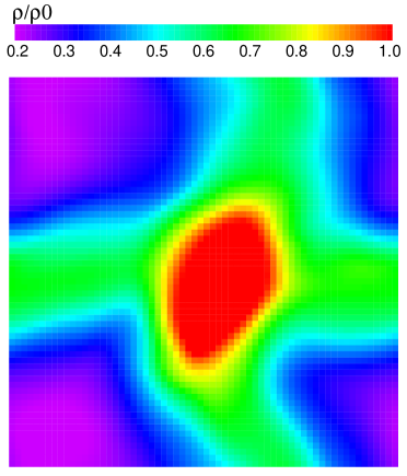
Figure 5: The density distribution for the $\gamma=50$ system at time $t=100$.

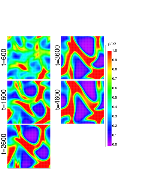
Figure 6: The density distribution for a large ($128\times 128$) system at several times during its evolution.

Figure 5 shows that our system develops a clustering instability as well. Note that the single cluster takes on a compact shape, which is surprising given that there is no surface tension in our model. If clusters are supposed to grow by accretion, then one would expect a ramified structure. This puzzle becomes clearer as we consider a larger system after further evolution. Figure 6 shows that clusters first form in these compact shapes, but as time goes on they reach out to their neighbors, stretching into the more stringlike forms seen in simulationgoldhirsch . In hindsight, we are able to see this behavior in the smaller system as well, where the single cluster interacts with itself through the periodic boundaries.

Figure 7: The width of the density distributions (i.e. $\rho_{max}-\rho_{min}$) for several values of $\gamma$, including the elastic case $\gamma=0$. Notice that the density distribution is collapsing to a delta function in the elastic case, approaching complete homogeneity, while the inelastic systems show broadening density distributions due to the clustering instability.

Finally, to demonstrate that this clustering instability is the result of the inelastic parameter, we compare the width of the density distribution for inelastic systems with the distribution for the elastic case $\gamma=0$ (Fig.7). In the absence of inelasticity, the density distribution collapses to a delta function, indicating complete homogeneity.

Our results show that the shearing and clustering instabilities, identified by Goldhirsch and Zanetti using a simplified version of the above equations, exist in the complete nonlinear granular hydrodynamic equations 1. Haff’s cooling law is obeyed in the limit of small inelasticity, but in general the instabilities become relevant before the system has a chance to completely homogenize. The power-law dependence of the onset time for these instabilities on the inelasticity, and the $-4/3$ exponent in particular, are interesting; we have not found any reference to these in the literature. Also interesting is the way in which these clusters develop from compact structures into networks which span the system. It is not clear whether an individual cluster begins to stretch out because of the proximity of its neighbors, or because of effects due to its increasing surface size. One can imagine that the behavior of this system could change as we alter the total amount of mass in the system.

We thank Professor Todd DuPont for his assistance in constructing our simulations, and Professors Heinrich Jaeger, Sidney Nagel, and Thomas Witten for helpful conversations. This work was supported by the Materials Research Science and Engineering Center through Grant No. NSF DMR 9808595.

References

- (1) J. Eggers, Phys. Rev. Lett. 83, 5322 (1999).
- (2) A. Kudrolli, M. Wolpert, and J.P. Gollub, Phys. Rev. Lett. 78, 1383 (1997).
- (3) J.S. Olafsen and J.S. Urbach, Phys. Rev. Lett. 81, 4369 (1998).
- (4) I. Goldhirsch and G. Zanetti, Phys. Rev. Lett. 70, 1619 (1993).
- (5) P.K. Haff, J. Fluid Mech. 134, 401 (1983); and J.T. Jenkins and S.B. Savage, J. Fluid Mech. 130, 187 (1983). More recently, J.J. Brey, M.J. Ruiz-Montero, and D. Cubero, Phys. Rev. E 60, 3150 (1999); T.P.C. van Noije and M.H. Ernst, Gran. Matt. 1, 57 (1998); J.J. Brey, J.W. Dufty, C.S. Kim, and A. Santos, Phys. Rev. E 58, 4638 (1998).
- (6) The temperature here is not thermal, but actually a measure of the local energy density that is not accounted for by the local flow velocity: . Apart from this equation, it is not necessary to assume that this quantity has any properties normally associated with temperature.
- (7) The question is similar to whether all of the physics of turbulence is captured by the Navier-Stokes equations, or whether one must, at some point, resort to a more microscopic theory.
- (8) P.K. Haff, J. Fluid Mech. 134, 401 (1983).
- (9) B. Kim and G.F. Mazenko, J. Stat. Phys. 64, 631 (1991). See also hill .
- (10) S.A. Hill and G.F. Mazenko, Phys. Rev. E 63, 031303 (2001). The actual structure of the free energy density (to which pressure is related by ) in our previous paper is more complex than what we use here, but it does possess the high-density barrier to account for the ultimate incompressibility of the grains.
- (11) Others have dealt with the high-density limit by having the viscosity diverge as the density approaches its maximum value. See, for example, W. Losert et al., Phys. Rev. Lett. 85, 1428 (2000).
- (12) Some details about our methods: (1) Our Runge-Kutta method includes an adaptive time step; it, however, is rarely activated since we use a default time step that is suitably small. (2) We offset the velocities from the other fields on the lattice such that the densities and temperatures may be considered to lie on the faces of the lattice while the horizontal (vertical) velocities lie on the vertical (horizontal) edges. (3) We have had great numerical difficulty with regions of very low density: such regions have a tendency to drift below zero density or generate large velocities in an unnatural fashion. We use an upwind technique to evaluate the equation , to prevent the density from becoming negative. In addition, we prevent mass from flowing out of any site with a density below some minimum value ().
- (13) Our dimensionless density should not be confused with the dimensionless packing fraction. For numerical convenience, our units of density have been scaled so that the random close-packed density corresponds to . We will refer often to the ratio to avoid confusion.
- (14) P. Deltour and J.-L. Barrat. Journal de Physique I 7: 137 (1997).
- (15) S. Luding and H.J. Herrmann. Chaos 9: 673 (1999).
- (16) X. Nie, E. Ben-Naim, S. Chen. arXiv:cond-mat/0209412 (2002).
- (17) S. McNamara and W.R. Young. Phys. Rev. E 53: 5089 (1996).