Nonlinear effects in E$\otimes(b_{1}+b_{2})$ Jahn-Teller model: Variational approach with excited phonon states and mode correlations.

Abstract

Interplay of nonlinear and quantum effects in the ground state of the E$\otimes(b_{1}+b_{2})$ Jahn-Teller model was investigated by the variational approach and exact numerical simulations. They result in the recognition of (i) importance of the admixture of the first excited state of the displaced harmonic oscillator of the symmetric phonon mode in the ground state of the system in the selftrapping-dominated regime; (ii) existence of the region of localized $b_{1}$-undisplaced oscillator states in the tunneling-dominated regime. The effect (i) occurs owing to significant decrease of the ground state energy on account of the overlapping contribution of the symmetric phonon mode between the states of the same parity. This contribution considerably improves variational results especially in the selftrapping-dominated regime. Close to the E$\otimes$e limit, the nonlinear effects of two-mode correlations turn to be effective due to the rotational symmetry of this case. In the tunneling-dominated regime the phonon wave functions behave like the strongly localized harmonic oscillator ground state and the effect (i) looses its significance.

pacs[63.20.Kr,31.30.Gs,71.70.Ej ]

I Introduction

Recently, revival of interest in two-level electron-phonon systems occurs owing to the experimental evidence that Jahn-Teller structural phase transition occurs in spatially anisotropic complex structures (fullerides, manganite perovskites, etc) [1]^,[2]^,[3]^,[4]^,[5].

JT model is a protopype model for phonon removing the degeneracy of electron levels [4]^,[1]. Current investigations were focused mainly on E$\otimes$e JT model with electron coupling to two degenerate intramolecular phonon modes, an antisymmetric and symmetric one with respect to the reflection.

The reflection symmetry of two-level electron-phonon models like the exciton and the dimer model with onsite electron coupling to one phonon mode implies nonlinear peculiarities of quantum nature [6]. For these models, Shore et al. [7] introduced variational wave function in a form of linear combination of the harmonic oscillator wave functions related to two levels of different parity with respect to the reflection. This picture can be understood in terms of two or more asymmetric local minima of the effective polaron potential (i.e. the potential energy expression for the trial wavefunction in the space of variational parameters). Here, respective ground state wave function can be approximated by a linear combination of two oscillators with parameters corresponding to these local minima and coupled by means of further variational parameters. This approach was shown to yield the lowest ground state energy for the two-level models [7]^,[8]. The peculiarities due to reflection phenomena occurred in the rotation-symmetric E$\otimes$e JT model [9] as well. Strongly localized non-displaced phonon (exotic) states appeared in the numerical spectra. They were considered useful for interpretation of the ”fast” component of luminiscence spectra. However, in order to respect the rotational symmetry of the $E\otimes e$ model the proper variational approach should be formulated in radial coordinates [10].

In crystals exhibiting high spatial anisotropy with tensor properties of bulk characteristics (e.g. perovskites, fullerids, etc.) the rotation symmetry of Jahn-Teller molecules is generally broken. Therefore, it is reasonable to investigate JT model assuming different coupling strengths $\alpha$ and $\beta$ for the onsite intralevel and interlevel electron-phonon couplings, respectively (E$\otimes(b_{1}+b_{2})$ model [1]). Such a model can be also considered as a generalization of the exciton-phonon or the dimer-phonon model assuming the electron tunneling to be phonon-assisted.

In order to understand the physical nature of the nonlinear effects we propose variational ansatz inspired by the shape of the numerical ground state wave function (Fig.1): the “principal” part of Gaussian character for both oscillators (in the absolute minimum of the nonlinear effective potential (Fig.1 of our previous paper [11] and Fig.2 of this paper) and a minor “reflective” part which corresponds to the another (local) minimum of the potential. For this minor part we consider the admixture of the first excited harmonic oscillator of the symmetric mode (rather than the only ground oscillator state, as it was commonly considered elsewhere). This admixture in the variation trial function leads to essential improvement of the results, as it will be shown in Sect. III.

Formulation of the variational ansatz and calculation of the ground state energy is presented in the Section II. In the Section III, analysis of the interplay of quantum effects and nonlinearity and related discussions as well as the reliability of different variational alternatives was investigated by comparison with results of exact numerical simulations.

II Variational wave function of the generalized JT model

We investigate local spinless double degenerate electron states linearly coupled to two intramolecular phonon modes described by Hamiltonian

$$H=\Omega(b_{1}^{{\dagger}}b_{1}+b_{2}^{{\dagger}}b_{2}+1)I+\alpha(b_{1}^{{\dagger}}+b_{1})\sigma_{z}-\beta(b_{2}^{{\dagger}}+b_{2})\sigma_{x},$$ (1)

where $\sigma_{x}=\left(\matrix{0,\ 1\cr 1,\ 0}\right)$, $\sigma_{z}=\left(\matrix{1,\ 0\cr 0,-1}\right)$ are Pauli matrices, $I$ is the unit matrix. This pseudospin notation refers to two-level electronic system, the Hamiltonian is thus $2\times 2$ matrix.

The antisymmetric phonon mode $b_{1}$ splits the degenerate unperturbed electron level ($j=1,2$) while the symmetric mode $b_{2}$ mediates the electron transitions between the levels. This latter term represents phonon-assisted tunneling, a mechanism of the nonclassical (nonadiabatic) nature as well as is the pure tunneling in related exciton and dimer models. Evidently, for $\beta=0$, the one-level Holstein model (1) is harmonic, while the coupling to the higher level ($\beta\neq 0$) is the origin of the strong nonlinearity in the phonon space as will be seen below.

For $\beta=\alpha$, the interaction part of (1) yields the rotationally symmetric $E\otimes e$ form [4] with a pair (an antisymmetric and a symmetric under reflection) of double degenerated vibrations.

The general case $\alpha\neq\beta$ exploited here breaks the common invariance of $E\otimes e$ Jahn-Teller model under the exchange of $1$ and $2$ phonons; in other words, the rotational symmetry of the Hamiltonian (1) is broken while the reflection symmetry is kept. This symmetry is inherent property of the Jahn-Teller model and it is crucial for the diagonalization of (1) and construction of the variational ansatz as it is evident from what follows.

Hamiltonian (1) can be diagonalized in the electronic subspace using the Fulton-Gouterman unitary operator [12]

$$U=\frac{1}{\sqrt{2}}\left(\matrix{1\ ,\ G_{1}\cr 1\ ,\ -G_{1}}\right),\quad G_{1}=\exp(i\pi b_{1}^{{\dagger}}b_{1}),$$ (2)

as follows

$$H_{FG}=UHU^{-1}=\Omega\left(b_{1}^{{\dagger}}b_{1}+b_{2}^{{\dagger}}b_{2}+1\right)+\alpha(b_{1}^{{\dagger}}+b_{1})I-\beta(b_{2}^{{\dagger}}+b_{2})\sigma_{z}G_{1}\equiv H_{ph}+H_{\alpha}+H_{\beta}.$$ (3)

The operator $G_{1}$ in (2) is the phonon reflection operator: $G_{1}(b_{1}^{{\dagger}}+b_{1})=-(b_{1}^{{\dagger}}+b_{1}),\ G_{1}^{2}=1$. We see that Fulton-Gouterman transformation reveals high nonlinearity in the system (term with $G_{1}$ in (3)), otherwise this nonlinearity was hidden in the initial Hamiltonian (1). Hamiltonian distincts from the exciton (dimer) by the phonon-2 assistance of the tunneling amplitude $\beta G_{1}$. The factor $G_{1}$ (2) represents continuous virtual emission and absorption of the phonons $1$ and mediates Rabi oscillations of the electron between the levels. These quantum oscillations are essentially the origin of the nonlinearity of the reflection symmetric model as will be seen below.

The full reflection operator is $G=G^{el}G_{1}$, where the electron reflection operator is defined by $G^{el}|1\rangle=|2\rangle$. Equivalently to the FG transformation one can exploit commutation of $G$ with Hamiltonian (1), $[H,G]=0$, so that the wave function of Hamiltonian (1) related to the representation of the inversion group $p=\pm 1$ is a linear combination of the base functions

$$|\Psi^{(p)}\rangle=\frac{1}{\sqrt{2}}(1+pG)|1\rangle|\phi^{(p)}\rangle,$$ (4)

where $G_{1}|\phi^{(p)}\rangle=|\phi^{(-p)}\rangle$. Hamiltonian (3) though diagonalized is no more reflection symmetric, but the interaction part is antisymmetric against reflection. As a consequence, in the limit $\alpha=\beta$ the rotation symmetry is broken. Therefore, use of the FG transformation in the case of E$\otimes$e JT is inappropriate: it breaks the symmetry which is necessary for the proper choice of the ground state in this case (see the discussion in the Conclusion).

Inserting the representation of the wave functions (5) into the Schrödinger equation related to (1) we are left with the Fulton-Gouterman equation

$$H_{FG}^{(p)}\phi^{(p)}=[\Omega\left(b_{1}^{{\dagger}}b_{1}+b_{2}^{{\dagger}}b_{2}+1\right)+\alpha(b_{1}^{{\dagger}}+b_{1})-p\beta(b_{2}^{{\dagger}}+b_{2})G_{1})]\phi^{(p)}=E^{(p)}\phi^{(p)},\ p=\pm 1.$$ (5)

It is evident that procedure yielding the set (5) is equivalent to the FG transformation yielding Hamiltonian (3) in the Pauli $2\times 2$ matrix representation. From the diagonalized form (5) we can see that $\beta$-coupling breaks the degeneration of two electron levels which do not have the same energy.

As it was pointed out to us, Hamiltonian (1) and, equivalently also (5) (and all the related quantities), are symmetric against simultaneous exchange of $p\leftrightarrow-p$, $\alpha\leftrightarrow-\beta$ and, ensuingly, in terms of parameters introduced later on, $\chi=\beta/\alpha\leftrightarrow 1/\chi$ and $\mu\equiv\alpha^{2}/\Omega^{2}\leftrightarrow\beta^{2}/\Omega^{2}$.

In what follows we shall investigate variationally the ground state ($p=1$) with lower energy only in the representation of Eq. (5).

In two-level electron-phonon systems with linear coupling the coherent phonon subsystem does not conserve the number of phonons. Therefore, the upper level will share partly the distribution of phonons even in the ground state. From this reason, the two-center wave function in the form of asymmetric nonunitary ansatz with a variational parameter $\eta$ proposed by Shore et al [7] and Sonnek et al [8] for exciton or dimer models coupled to one phonon mode

$$|\Psi^{(1)}\rangle=\frac{1}{\sqrt{C}_{0}}(1+\eta G)|1\rangle|\phi^{(1)}\rangle,$$ (6)

($C_{0}$ is a normalization constant) was proved to yield better (lower) estimation of energy of the ground state [7]^,[8] when compared with the eigenfunction $|\phi^{(1)}\rangle$ of $H_{FG}$ (5).

Our present suggestion of the variational ansatz for the ground state is motivated by the numerical solution for the wave function to the diagonalized Eq. (5). In the following numerical and analytical calculations it is convenient to use two basic parameters: the asymmetry parameter $\chi=\beta/\alpha$ and the effective coupling strength $\mu=\alpha^{2}/2\Omega^{2}$. The wavefunctions for the strong coupling $\mu=2$ and $\chi=0.9$, $\chi=1$, and $\chi=1.5$ are given in Figs. 1a,b,c (the standard numerical simulation procedure is outlined in the next Chapter) where the wavefunctions are depicted in the coordinate representation in the space of two phonon oscillators $Q_{1}\otimes Q_{2}$. Three distinct forms of the phonon solutions correspond to small, intermediate and large values of the parameter $\chi$.

Fig. 1a represents the “selftrapping” region in which contribution of the electron transitions between the levels (assisted by the oscillator 2) is small. Here the main Gaussian of the wave function $\phi^{+}(Q_{1})$ at negative values of $Q_{1}$ ($p=+1$) is accompanied in the $Q_{1}$-subspace by the reflective part $\eta\phi^{-}(-Q_{1})$ corresponding to $p=-1$ parity which have already inspired the introduction of the nonunitary ansatz (6) representing the minor reflection respective to the axis $Q_{1}=0$ [7]. However, in Fig. 1a, the admixture of the first excited state of the oscillator 2 (coordinate $Q_{2}\approx 0$) of the parity $p=-1$ (displaced to the right to $Q_{1}>0$) can be recognized, while for $p=+1$ both oscillators (region $Q_{1}<0$) remain in the Gaussian ground state. The variational treatment which is the topic of present paper aims mostly at capturing the situation of Fig. 1a as adequate as possible.

In Fig. 1b ($\chi=1$) which represents the case of E$\otimes$e Jahn-Teller molecule, the rotational symmetric nature of the ground state at $\chi=1$ is easily recognizable. We mention by passing that an ideal rotation symmetry of the phonon wavefunction (“mexican hat”[4]) which might be expected in the adiabatic case (that is that of big $\mu$) of a rotationally symmetric problem can not be reached even for very large $\mu$, as it was explained in detail by Eiermann et al[9]. For the symmetric $E\otimes e$ Jahn-Teller case we have merely an approximation to the “mexican hat” wavefunction profile spoiled by the non-zero angular momentum part which prevents the profile to show the complete rotational symmetry. This picture combines in it the features of self-trapping (Fig. 1a) and tunnelling (Fig. 1c) cases. The region close to E$\otimes$e Jahn-Teller case appears also to show the most serious discrepancies of the variational treatment.

Fig. 1c represents another limit case - that of large values of $\chi$ corresponding to the (quantum) region of dominated phonon-assisted tunnelling. There the Gaussian form of the wave function is retained, although the second oscillator is displaced towards $Q_{2}>0$, while phonons 1 remain undisplaced (the Gaussian is centered at $Q_{1}\approx 0$).

In Figs. 2a,b,c, we sketched three shapes of the effective potential (energy expression from the trial functions) controlled by the displacement parameters $\gamma_{1}$ and $\gamma_{2}$ only which refer to the variants of the wave functions in Figs. 1a,b,c, respectively.

Thus, guided by Fig. 1a, the variational wave function can be proposed in the following nonunitary form

$$\Psi=\frac{1}{\sqrt{C}}\left[\phi_{0}^{(+)}(\gamma_{1},\gamma_{2},r_{1},r_{2},\lambda)+\eta_{1}\phi_{0}^{(-)}(-\gamma_{1},\gamma_{2},r_{1},r_{2},-\lambda)+\eta_{2}\phi_{1}^{(-)}(-\gamma_{1},\gamma_{2},r_{1},r_{2},-\lambda)\right]$$ (7)

where $7$ variational parameters $\gamma_{i}$, $r_{i}$, $\eta_{i}$, and $\lambda$ are introduced and defined below.

Phonon wave functions $\phi_{i}^{(\pm)},\ i=0,1$, are supposed to be squeezed coherent and correlated oscillators produced applying the set of generators on the phonon vacuum state as follows:

$$\phi_{0}^{(\pm)}(\gamma_{1},\gamma_{2},r_{1},r_{2},\lambda)=D_{1}(\pm\gamma_{1})S_{1}(r_{1})D_{2}(\gamma_{2})S_{2}(r_{2})S_{12}(\pm\lambda)|0\rangle,$$ (8)

$$\phi_{1}^{(-)}(\gamma_{1},\gamma_{2},r_{1},r_{2},\lambda)=D_{1}(-\gamma_{1})S_{1}(r_{1})D_{2}(\gamma_{2})S_{2}(r_{2})S_{12}(-\lambda)b_{2}^{{\dagger}}|0\rangle,$$ (9)

($|0\rangle$ is the phonon-$1,2$ vacuum state; indices $0,1$ at $\phi_{0},\phi_{1}$ denote the ground and the first excited state of displaced phonons, respectively).

Here we defined the generators of variational displacements $\gamma_{i}$

$$D_{i}(\gamma_{i})=\exp[\gamma_{i}(b_{i}^{{\dagger}}-b_{i})],$$ (10)

and those of squeezings parametrized by $r_{i}$

$$S_{i}(r_{i})=\exp[r_{i}(b_{i}^{{\dagger}2}-b_{i}^{2})]$$ (11)

which are functions of variational parameters of displacement $\gamma_{i}$ and squeezing $r_{i}$ for $i=1,2$. In Eq. (5) the phonon modes $1$ and $2$ appear coupled in a highly non-linear way (through the term with $\beta$), therefore one also includes into the ansatz (7) the mode correlation generator

$$S_{12}(\lambda)=\exp[\lambda(b_{1}^{{\dagger}}b_{2}^{{\dagger}}-b_{1}b_{2})]$$ (12)

with the correlation variational parameter $\lambda$.

The functions $\phi_{0}^{(+)}$ and $\eta_{1}\phi_{0}^{(-)}$ in (7-9) represent displaced and squeezed oscillators in $Q_{1}\times Q_{2}$ space whose weight is shifted to the points $(+\gamma_{1},+\gamma_{2})$ and $(-\gamma_{1},+\gamma_{2})$ respectively (see Fig.1a); The function $\phi_{0}^{-}$ is merely the reflection of $\phi_{0}^{(+)}$ weighted by $\eta_{1}$: $\phi_{0}^{(-)}=G_{1}\phi_{0}^{(+)}$ (see (4-6)).

The function $\phi_{1}^{(-)}$ is the excited oscillator $b_{2}^{+}|0>_{1}|0>_{2}$ displaced likewise $\phi_{0}^{(-)}$ into the point $(-\gamma_{1},\gamma_{2})$ of $Q_{1}\otimes Q_{2}$ space and squeezed as well (by parameters $r_{1},r_{2}$) with weighting parameter $\eta_{2}$. In what follows we show that introducing this admixture of the excited state of the oscillator-2 in (7) essentially improves variational results.

The last variational parameter $\lambda$ enters in generators $S_{12}(\pm\lambda)$ which mix phonon modes together; this can be visualized as effective rotation of the two-dimensional Gaussian in the plane $(Q_{1},Q_{2})$; different signs $\pm\lambda$ keep trace of the reflection symmetry against the line $Q_{1}=0$ (it is best seen from Fig.1b that left and right “hills” should rotate in the opposite directions).

The complete expression for the mean value of the Hamiltonian $H=H_{ph}+H_{\alpha}+H_{\beta}$ (3) in the state (7)-(12) is given in Appendix B. A useful representation of that expression can be the following decomposition which separates the contributions of “ground” and “excited” parts of trial functions:

$$\langle H\rangle=\frac{1}{C}\left[\langle(\phi_{0}^{{\dagger}}+\eta_{2}\phi_{1}^{(-){\dagger}})H(\phi_{0}+\eta_{2}\phi_{1}^{(-)})\rangle\right]$$ (13)

$$=\frac{1}{C}\left[\langle\phi_{0}^{{\dagger}}H\phi_{0}\rangle+2\eta_{2}\langle\phi_{0}^{{\dagger}}H\phi_{1}^{(-){\dagger}}\rangle+\eta_{2}^{2}\langle\phi_{1}^{(-){\dagger}}H\phi_{1}^{(-)}\rangle\right],$$ (14)

where $\phi_{0}=\phi_{0}^{(+)}+\eta_{1}\phi_{0}^{(-)}$, and

$$C=\left(1+\eta_{1}^{2}+2\eta_{1}\varepsilon+\eta_{2}^{2}\right),\quad\varepsilon=\frac{\exp\left(-\frac{2\tilde{\gamma}_{1}^{2}}{\cosh 2\lambda}\right)}{\cosh 2\lambda}.$$ (15)

The effective Hamiltonian (14) involves a highly nonlinear interplay of the variational parameters: the admixture of the state $\phi_{1}^{(-)}$ contributes by the terms due to overlapping of the ground and first excited state of the oscillator $\propto\eta_{2}$ and by its own excitation energy $\propto\eta_{2}^{2}$.

In what follows, we investigate joint effects of quantum fluctuations and nonlinearity in the ground state of (14) by minimalization of the energy expression with respect to involved VPs $\gamma_{1},\gamma_{2},r_{1},r_{2},\lambda,\eta_{1},\eta_{2}$. Parameters of the displacement $\gamma_{1},\gamma_{2}$ are defined by the displacement generators $D_{i}(\gamma_{i})$ (10), parameters of squeezing $r_{i}$ by the generators of squeezing $S_{i}(r_{i})$ (11), parameter of the mode correlation $\lambda$ by the generator of the correlation $S_{12}(\lambda)$ (12) and the parameters of asymmetry $\eta_{1},\eta_{2}$ by the linear combination (7).

III Interplay of quantum and nonlinear effects in selftrapping and tunneling

As it was shown in the last Section, the reflection symmetry hidden in the original Hamiltonian reveals in Eq. (5) due to the diagonalization by FG transformation in a highly nonlinear way. This nonlinearity implies new purely quantum region of the ground state with strong mixing of the nonlinearity and quantum fluctuations. There are several mechanisms supporting the quantum (nonadiabatic) fluctuations:

In the present model the relevant nonadiabaticity parameter is the ratio of the frequency and the coupling parameter $\Omega/\alpha$. The ratio of the polaron energy $\frac{\alpha^{2}}{\Omega}$ and of the frequency $\Omega$, $\alpha^{2}/\Omega^{2}=2\mu$ is a measure of the competition between the classical (polaron selftrapping) and quantum effects due to zero energy fluctuations. The quantum effects related to $\Omega$ are thus relevant at weak couplings $\mu$.

The competition between the selftrapping ($\alpha$) and tunneling ($\beta$) terms results in occurrence of two regions of the ground state: In the phase plane $\chi$, $\mu$, the ground state exhibits two phases separated by the crossover line close to $\chi=1$ (Figs. 3, 4, 5, see also pertaining discussion in our earlier paper [11]). It means that the effective polaron potential exhibits two competing minima (Fig. 2a) governed by the model parameters $\mu$ and $\chi$. The minima coincide within the border of the regions lying close to the line $\chi=1$ (Fig. 2b). The phase $\chi<1$ is selftrapping dominated, with quantum fluctuations reflected in parameters $r_{1},r_{2},\lambda,\eta_{i}$. The phase $\chi>1$ is the phonon 2-assisted tunneling dominated region with continuous virtual emission and absorption of phonons $1$. This phonon-1 exchange couples the levels within one minimum displaced merely by $\gamma_{2}$ due to the phonons 2. This minimum is much more sensitive to the change of model parameters $\mu,\chi$ as well as to quantum fluctuations reflected in $r_{1},r_{2}$, $\lambda$ and insensitive with respect to $\eta_{i},$ while $\eta_{i}\approx 0$.

From the electronic point of view, the electron in the selftrapping dominated region is trapped by the phonons $1$, but due to the interactions mediated by the phonons 2 it can tunnel to the higher level. Then, owing to the reflection symmetry of the phonons 2, continuous oscillations of the electron at simultaneous virtual emission and absorption of phonons 1 occur. These oscillations couple the levels and thus the electrons into pairs localizing them in one minimum (Fig. 2c). This mechanism was described in a recent paper [11] for a one-dimensional lattice model.

An insight to the importance of different variational parameters can be gained by analytical minimalization of Hamiltonian (14) in various approximations. Numerical considerations show that contributions from the quantum parameters $r_{i},\eta_{i},\lambda$ are at least by an order smaller than those from the classical parameters. Including also $\eta_{2}$, we get approximately ($\Omega=1$):

$$\langle H\rangle=\gamma_{1}^{2}+\gamma_{2}^{2}+1+2\alpha\gamma_{1}\frac{(1-\eta_{2}^{2})}{(1+\eta_{2}^{2})}-2\beta\gamma_{2}\varepsilon+2\eta_{2}(\gamma_{2}\varepsilon-\beta).$$ (16)

Assuming all nonadiabatic parameters small and minimalizing (16) we get approximately

$$\gamma_{1}\left(1+4\beta^{2}\varepsilon^{2}\right)=-\alpha\,,\quad\gamma_{2}=\beta\varepsilon\,,$$ (17)

where $\varepsilon\propto\exp(-2\gamma_{1}^{2})$ (15). From these equations, approximate expressions for both regions (small and large $\chi$) are summarized below:

In the “selftrapping” region $\alpha>\beta$ ($\chi<1$) there is $\varepsilon\ll 1$ and we get:

$$\gamma_{1}\simeq-\alpha\,,\quad\gamma_{2}=\beta\varepsilon\ll 1,$$ (18)

(that is small $\gamma_{2}$ and large negative $\gamma_{1}$); In the framework of this approximation (taking also $\eta_{2}$ small) respective ground state energy in the selftrapping region results in

$$E_{G}^{\alpha}\approx 1-\frac{\alpha^{2}}{1+8\beta^{2}\exp(-4\alpha^{2})}-\beta^{2}\exp(-4\alpha^{2}).$$ (19)

For the tunnelling dominated region, vice versa:

$$\gamma_{1}\simeq-\frac{\alpha}{1+4\beta^{2}}\ll 1\,,\quad\varepsilon\simeq 1-2\gamma_{1}^{2}\,,\quad\gamma_{2}=\beta\varepsilon\simeq\beta.$$ (20)

In this case the ground state energy is approximated by

$$E_{G}^{\beta}\approx 1-\frac{\alpha^{2}}{1+8\beta^{2}}-\beta^{2}.$$ (21)

Comparing both ground state energies (19) and (21) we observe the asymmetry against the exchange of the $\alpha$ and $\beta$ of both results due to the screening of the tunneling term $\propto\beta^{2}$ by $\varepsilon=\exp(-2\gamma_{1}^{2})$ which is either vanishingly small (18) or $\propto 1$ (20). Evidently, it is caused by the presence of the nonlinear $G_{1}$ factor in the Fulton-Gouterman Hamiltonian (3) or (5).

Let us examine more thoroughly the parameter $\eta_{2}$ representing the relative weight of the “excited” admixture. Qualitatively important features brought by the Ansatz (7) can be found analytically merely from the simplified version of the Hamiltonian (14) and (45)-(59) with only displacements $\gamma_{i}$ and $\eta_{2}$.

The equation for optimized value $\eta_{2}$ for both regions reads exactly as

$$\eta_{2}(1-4\alpha\gamma_{1})-(1-\eta_{2}^{2})\beta(1-\varepsilon^{2})=0\,;$$ (22)

Inserting there the above expressions for $\gamma_{i}$ (17-20) we get:

• for the selftrapping region

  $$\eta_{2}^{(I)}\simeq\frac{\beta(1-\varepsilon^{2})}{1+4\alpha^{2}},$$ (23)

• for the tunnelling region

  $$\eta_{2}^{(II)}\simeq\frac{4\beta\gamma_{1}^{2}}{1-4\alpha\gamma_{1}}\simeq 0\,,$$ (24)

$\gamma_{1}$ given by (20).

This analytical estimation shows that the admixture of the excited $2$-phonons should play the most important part in the selftrapping region only; This conclusion is in the complete accordance with the shapes of the wave functions for both regions (Figs 1a, 1c), as well as with further exposed results of minimalization of variational energies (Figs. 3-5).

Further, exploiting the influence of $\lambda$ and $\eta_{1}$ separately (using (14), Appendix B and (18) for $\chi<1$ ), we get estimations:

$$\sinh(2\lambda)\simeq-2\beta\varepsilon\gamma_{1}\simeq 4\chi\mu\exp(-4\mu),\quad\eta_{1}\simeq-\frac{\beta\gamma_{2}}{\alpha\gamma_{1}}\simeq\chi^{2}\exp(-4\mu),$$ (25)

where $\mu=\alpha^{2}/2\Omega^{2}$ was defined at the beginning of the Section III. as the parameter of the effective interaction. (The first dependence of (25) is recognizable on Fig. 6 and will be discussed later in relation to the necessity of accounting for mode correlation).

We calculated then the optimized values of the variational parameters finding numerically the minimum of the energy functional in different approximations - starting from the most complicated case of complete expression (Appendix B) with 7 parameters included and ending with the adiabatic ansatz with the displacements $\gamma_{1},\gamma_{2}$ only.

In order to check the validity of the variational calculations we performed also the numerical diagonalization of the Hamiltonian in the phonon-$1,2$ space. We truncated the (infinite) phonon space by $N_{1}$ 1-phonon states and $N_{2}$ 2-phonon states, thus the state vector is $N_{1}\times N_{2}$ dimensional. As numerical diagonalization results show, about 20-50 phonon states are sufficient for convergence. In Figs. 3 to 5 we also show the results of numerical diagonalization of Hamiltonian matrix as function of $\chi$ for $\mu=0.5$, $\mu=1$ and $\mu=4$. In the first two cases we took 20$\times$20 state vector, while in the latter case to achieve satisfactory convergence (especially for the tunneling-dominated region when $\chi>1$) we had to increase the number of phonons-2 up to 50.

The two energy curves from exact numerical solution and “adiabatic” variational treatment present correspondingly the lower and upper bound for variationally calculated energy, thus any reasonable variational results should lie between these bounds, and reliability of a variation ansatz for a given parameter region can be judged according to how close the corresponding ground state energy is to these limits (Figs. 3-5).

We limited ourselves by showing merely some crossections of the plane $\chi,\mu$ which seem to be typical in discussing the validity of the variational approach vs “true” solution via numerical diagonalization in the phonon subspace. From Figs. 3b to 5b showing the differences between “variational” and “exact” energy for various variational approximations it is seen that while the curves with all parameters $\eta_{i},\lambda,r_{i},\gamma_{i}$ included give minimal discrepancy (which is evident, since increasing the number of variational parameters within the same trial function class leads to improving the results), the maximal discrepancy, and hence the maximal effect of additional parameters $\eta_{i}$, $\lambda$ is observed near the line $\chi\simeq 1$, this region of observed maximal discrepancy being shifted to the point $\chi=1$ with growing $\mu$.

From the results of numerical minimalization of the variational expressions for energy (see Fig. 3-5) one can see that the “excitation-reflection” ansatz (ERA) (7) ($\eta_{2}$ included) results in fascinating improvement of the variational simulation of the problem in comparison with the “simple reflection” ansatz (SRA) ($\eta_{1}$ only); especially it is evident from Figs. 3b, 4b, 5b, where the differences between variational and “exact” energies are plotted. Although this ansatz can be to a larger extent inspired by merely the shape of the wave function (Fig. 1a) one might wonder that the ansatz containing an excited oscillator as the “reflective” part of the trial function lowers the total energy of the system in comparison with the ansatz containing the “zero” state of the oscillator ($\eta_{2}=0$). An insight to better understanding this phenomenon can be gained examining the variational energy expression (14), (45)-(59). The energy can be split into three parts representing respectively the energy of the “main” Gaussian, that of the reflection part and “overlapping” exchange terms (those containing $\eta_{i}^{0}$, $\eta_{i}^{2}$, $\eta_{i}^{1}$ respectively). Indeed when we switch from SRA towards ERA the energy of the reflection part is increased by $\sim\eta_{2}^{2}$ by virtue of one extra displaced “phonon” (59); But, if one compares the overlapping terms for both expressions (below) one can see that it is the overlapping term of ERA (53), (26) which significantly decreases the overall energy, while the respective overlapping term of SRA (45), (27) contributes only slightly.

The main contribution to the overlapping integral is contained in the term $\ \langle\Phi_{0}(\gamma_{1})|Q_{2}G|\Phi_{1}(-\gamma_{1})\rangle=\langle\Phi_{0}(\gamma_{1})|Q_{2}|\Phi_{1}(\gamma_{1})\rangle\sim 1$ ($Q_{2}$, second phonon coordinate, is a short-hand for $(b_{2}^{+}+b_{2})$); other terms contain a small “overlapping” factor $\varepsilon\sim\exp(-2\gamma_{1}^{2})$. Using rough estimations (the same as those leading to (17)) we get following expression for the “overlapping” part of energy in the ERA:

$$E_{l}\simeq-2\eta_{2}(\beta e^{2r_{2}}\cosh\lambda+\alpha e^{2r_{1}}\sinh\lambda)\sim-2\eta_{2}\beta\,,$$ (26)

(this expression is valid for the region $\chi<1$). In (26), it is the $\beta$-term which yields the main contribution.

As for the SRA, its counterpart reads as $\langle\Phi_{0}(\gamma_{1})|Q_{2}|\Phi_{0}(-\gamma_{1})\rangle$ and vanishes due to symmetry, leaving us only smaller terms $\propto\varepsilon$,:

$$E_{l}\simeq-4\beta\eta_{1}\varepsilon\,$$ (27)

(the higher order terms $\sim\varepsilon^{2}$, $\varepsilon^{2}\eta$ etc. are omitted).

Comparing these expressions we can see that ERA yields better use of the reflection symmetry property of Hamiltonian contributing greatly to the overlapping integral (to the negative exchange energy) while for the SRA this principal contribution vanishes merely because of symmetry, leaving us with minor contributions $\sim\varepsilon$ only, thus there the whole idea of the reflective ansatz losses much of its effectivity.

This effect of lowering energy in the excitation ansatz due to overlapping finds its origin in the presence of phonon-$2$ assistance. In the dimer or exciton models instead of $\beta\hat{Q_{2}}\sigma_{x}$ term of the model Hamiltonian (1) there stands merely $\Delta\sigma_{x}$ with the constant $\Delta$[8] and this principal part of the exchange energy (overlapping integral) for the excitation ansatz vanishes.

The very general impression from Figs 3-5 (b) makes us to state that introducing nonunitary parameters ($\eta_{i}$) essentially improves the variational treatment for the self-trapping region; In the tunnelling region merely Gaussian expressions for displaced oscillators with squeezing (parameters $r_{i}$) gives us a satisfactory fit. Indeed, as it was demonstrated from analytical estimations and as it is seen from Figs. 1 a,c, the admixture of reflection part is relevant rather for selftrapping region where this form of the trial function is the best choice.

However, the closer we are to the intermediate region between selftrapping and tunnelling phases, the stronger are discrepancies for all curves. As it is seen from Fig.1 b it is the case where the wavefunctions display their radial symmetric structure. Examining on Figs. 3-5 the curves corresponding to variational ansatzes with or without mixing parameter $\lambda$ we see that this parameter essentially lowers the energy exactly in the region of $\chi\simeq 1$. It is worth comparing Fig. 3 for $\mu=0.5$ (weak coupling) with Figures 4 and 5 ($\mu=1,\mu=4$), both representing strong couplings. We see immediately that the coupling parameter $\lambda$ gains importance rather for small couplings where it improves the results for wider range of $\chi$, and not only for $\chi\simeq 1$.

Fig. 6 where we plotted the differences of the variational energy calculated with and without taking into account the mode correlation $S_{12}(\lambda)$ illustrates this statement (see also (20)) by showing the regions of importance of the correlation parameter $\lambda$ in the whole plane ($\chi,\mu$). The mode correlation represented by $\lambda$ (Fig. 6) appears to be by one order larger than the contribution of the competing nonlinearity due to the reflection level mixing $\eta_{1}$. The correlation $\lambda$ is most effective for weak effective couplings $\mu$ at $\chi\simeq(0.5,1.5)$ where it competes the selflocalization in support of the tunneling phase. For large $\mu$ it contributes only very close to $\chi=1$, where it reveals a maximum for all $\mu$. This is quite understandable if we note that introducing $S_{12}(\lambda)$ (12) means effective rotation of trial functions (displaced Gaussians) in the plane $Q_{1}\otimes Q_{2}$, and $\phi^{+}(\lambda)$, $\phi^{-}(-\lambda)$ are rotated in the opposite directions symmetrically with respect to the line $Q_{1}=0$, which indeed repeats Fig.1b, fitting the rotation symmetry features. This degree of freedom allows to represent the picture of the wave function especially in the transition region where selftrapping and tunnelling regions are mixed together and are hardly distinguishable, which is the case of weak couplings. At strong couplings those regions are more pronounced, the border between them is sharper; in this case the parameter $\lambda$ looses its importance with exception of the vicinity of $\chi\simeq 1$ (Fig. 6).

In the case of omitting $\lambda$, from (40)-(59) one can see that the optimized value $r_{2}=0$, i.e. the contribution due to $r_{2}$ in (40) is mediated merely by the correlation $\lambda$. For $\lambda\neq 0$, the squeezing $r_{2}$ significantly interplays with $r_{1}$ especially for small $\mu$ and $\chi\approx 1$, as it brings almost half of the contribution of $r_{2}$. This effect was omitted in the variational treatment of E$\otimes$e model by Lo[13]. Some authors disregarded this circumstance setting $r_{1}=r_{2}$ for simplicity, but omitting the mode correlation ($\lambda$) which is therefore not selfconsistent.

In the lattice case, the coupling with the lattice is represented by a transfer term in the Hamiltonian of the order of magnitude of the bandwidth $T$[11]. When $T$ is sufficiently large so that the “transfer” part of the energy is comparable to the “local” energy contribution, the effect of $\eta_{1}$ is considerably stronger, and we do not observe suppression caused by introducing extra correlation between phonon modes (that is an analogue to the parameter $\lambda$). The phonon-$1,2$ correlation in the lattice case is of smaller order of magnitude than the contributions from the transfer terms (respectively of the order $\beta\exp(-\gamma_{1}^{2})$ and $T$). Because of that introducing the correlation VP in the lattice case does not yield considerable improvement of the results.

IV Conclusion

Hamiltonian (3) allows us to distinguish two competing regimes of the electron-phonon system according to the relations of the parameters specifying (a) selflocalization $\alpha$ vs quantum fluctuations $\Omega$ and (b) tunneling $\beta$ vs selflocalization $\alpha$. Then, in terms of the relevant parameters $\mu=\frac{\alpha^{2}}{2\Omega^{2}}$ (effective interaction) and $\chi=\frac{\beta}{\alpha}$ (asymmetry), two quantum regions can be identified: (i) $\mu\leq 0.5$ and (ii) $\beta/\alpha\geq 1$. In these regions the quantum fluctuations are most pronounced and variational ansatz which pretends to be the most suitable should fit there the numerical data at best. Our choice of the wave function (7)-(12) covers both regions in a complementary way: while the choice of ERA with the admixture of the excited state of the symmetric phonon mode weighted by $\eta_{2}$ and including the mode correlation $\lambda$ improves greatly the variational results in the selftrapping region, $\chi\leq 1$, in the whole range of $\mu$ (Figs. 2, 4, and 5), with increasing $\mu$ effectiveness of all quantum variational parameters vanishes except of $\eta_{2}$ (Figs. 4 and 5). In the tunneling region, $\chi>1$, the choice of ERA looses its justification in benefit of SRA, while all the remaining parameters keep their effectiveness even for large $\mu$ (Figs. 4 and 5).

The cooperative effect of the reflection (antisymmetric phonon mode) and of the assistance of the symmetric mode in the tunneling results in a nonlinear interplay of both modes. It consists in the competition between the negative contribution of the overlapping of the wave functions of different parity with respect to the reflection and the increase of excitation energy of the respective mode. This concept leads to the effective energy decrease of the excited symmetric reflected mode (ERA) rather than of its ground state (SRA).

The complex nonlinear interplay of the modes was elucidated by exact numerical diagonalization of Hamiltonian (3): in fact, we took inspiration for ERA from the exact ground state wave function for $\alpha\geq\beta$ (Fig. 1a). It suggested presence of admixture of the first excited oscillator state of the symmetric mode in the reflected part of the wave function. In the case of $\alpha<\beta$, the numerical wave function exhibited only a single symmetric peak of a well defined harmonic oscillator. The peak was located close to the center of the reflection symmetry $Q_{1}=0$ but displaced by the phonons $2$. It corresponded to a new minimum of the effective potential which opened due to the ”bond selflocalization” on account of the joint effect of both modes (Fig. 2c). Note that these states are well localized, in the contrast to the states in the “selftrapping” region. It is interesting to mention in this context a special class of states in the excited spectra of J-T models which were called “exotic states” [6, 9] and were characterized by a pronounced localization of the corresponding phonon mode. These states in the excitation spectra can be explained as the consequence of the energy resonance and hence the tunnelling between two wells of the effective potential (visualized, e.g., on Fig. 2) which suggested opening of the additional potential well in the position $\gamma_{1}\simeq 0$ where the exotic mode is to be localized. Although in the present paper we investigated merely the ground state of the model, we can see that our localized modes in the tunnelling dominated region ($\chi>1$) have essentially the same origin (the “localized” minimum at zero displacement along $Q_{1}$ of the effective potential) and bear interesting resemblance to the Wagner’s exotic states. In support of this statement the full spectrum of the phonon states, and not the ground one only should be examined, but this problem merits a special paper. We just mention now our own results on numerical calculation of the energy spectrum for the excited modes in the tunnelling region which show specific periodic (in model parameter $\mu$) chaotic “windows” especially for higher modes. This periodicity in the coupling strength, which we at the very beginning scaled by the phonon frequency $\Omega$ clearly indicated the resonance behaviour, i.e. occasional coincidence of two incommensurable characteristic frequencies of the system whose nature can be identified with the origin of Wagner’s resonant exotic states. For low lying modes like those of the ground state this behaviour is not so pronounced, but merely its traces are also recognizable.

The results exposed above, especially when speaking about the validity of the variational approach chosen, are most adequate far from the rotationally symmetric Jahn-Teller case ($\alpha=\beta$, or $\chi=1$) which was to be expected on basis of the comment to the FG transformation in the Section II. In this case one gets an almost degenerated degree of freedom in the space of variational parameters; namely, if we introduce an analogue of the polar coordinates in the phonon-1,2 space (as some authors[4]^, [9]^, [10] do), certain degeneracy of the energy profile over the angular coordinate would be observed and thus this angular parameter should have been excluded from being variated. (Strictly speaking, the angularly degenerated true “mexican hat” appears only in adiabatic approximation[4]). The authors exploiting various variational treatments disregarding this circumstance must have encountered such problems for the E$\otimes$e Jahn-Teller case. However, these inconsistencies become crucial rather at big coupling strength $\mu$, e.g., Fig. 4, 5). However, the rotational symmetry can be to some extent retained even within the formalism of rectangular $Q_{1}\otimes Q_{2}$ space by introducing the mode mixing parameter $\lambda$ which gains its significance especially in the region of weak coupling effectively spanning both regions (Fig. 6). The variational approach exploiting essentially the rotational symmetry of the model should present a complementary description suitable in the vicinity of $\chi=1$, the whole problem however being a subject of our further considerations.

The support from the Grant Agency of the Czech Republic of our project No. 202/01/1450 is highly acknowledged. We thank also the grant agency VEGA (No. 2/7174/20) for partial support.

Appendix A.

We have used following formulas for $D_{i}$, $S_{i}$, and $S_{12}$ defined by (10)-(12) which can be found elsewhere [14]^,[15]:

$$D_{i}(\gamma_{i})^{-1}b_{i}D_{i}(\gamma_{i})=b_{i}+\gamma_{i},\ i=1,2,$$ (28)

$$D_{1}(\gamma_{1})S_{1}(r_{1})=S_{1}(r_{1})D_{1}(\tilde{\gamma}_{1}),\ \tilde{\gamma}_{1}=\gamma_{1}e^{-2r},$$ (29)

$$S_{i}^{-1}(r_{i})b_{i}S_{i}(r_{i})=b_{i}\cosh 2r_{i}+b_{i}^{{\dagger}}\sinh 2r_{i},$$ (30)

$$S_{12}^{-1}(\lambda)b_{1}S_{12}(\lambda)=b_{1}\cosh\lambda-b_{2}^{{\dagger}}\sinh\lambda,$$ (31)

$$\langle 0|S_{1}^{{\dagger}}(r_{1})D_{1}^{{\dagger}}(\gamma_{1})\exp(\lambda b_{1}^{{\dagger}})\rangle=\frac{1}{(\cosh 2r_{1})^{1/2}}\times$$ (32)

$$\times\exp\left[\frac{\lambda^{2}}{2}\tanh(2r)-\lambda\gamma_{1}(\tanh 2r-1)+\frac{\gamma_{1}^{2}}{2}(\tanh 2r-1)\right],$$ (33)

$$\langle 0|S_{1}(r)D_{1}(\gamma_{1})b_{1}^{{\dagger}m}\rangle=\frac{d^{m}}{d\lambda^{m}}\langle 0|S_{1}(r_{1})D_{1}(\gamma_{1})\exp(\lambda b_{1}^{{\dagger}})\rangle|_{\lambda=0},$$ (34)

$$S_{12}(\lambda)=T^{{\dagger}}\left(\frac{\pi}{4}\right)S_{1}\left(\frac{\lambda}{2}\right)S_{2}\left(-\frac{\lambda}{2}\right)T\left(\frac{\pi}{4}\right),$$ (35)

$$T(\delta)=\exp\left(\delta(b_{1}^{{\dagger}}b_{2}-b_{1}b_{2}^{{\dagger}})\right)$$ (36)

$$T\left(\frac{\pi}{4}\right)\left(\matrix{b_{1}\cr b_{2}}\right)T^{{\dagger}}\left(\frac{\pi}{4}\right)=\frac{1}{\sqrt{2}}\left(\matrix{b_{1}-b_{2}\cr b_{1}+b_{2}}\right),$$ (37)

$$T^{{\dagger}}|0\rangle=T|0\rangle=|0\rangle.$$ (38)

Appendix B.

$$\langle H\rangle=\frac{1}{C}\left[\langle(\Psi_{0}^{(+){\dagger}}+\eta_{1}\Psi_{0}^{(-){\dagger}})H(\Psi^{(+)}_{0}+\eta_{1}\Psi^{(-)}_{0})\rangle+2\eta_{2}\langle\Psi_{0}^{(+){\dagger}}H\Psi^{(-)}_{1}\rangle\right.$$ (39)

$$\left.+2\eta_{1}\eta_{2}\langle\Psi_{0}^{(-){\dagger}}H\Psi^{(-)}_{1}\rangle+\eta_{2}^{2}\langle\Psi_{1}^{(-){\dagger}}H\Psi^{(-)}_{1}\rangle\right]$$ (40)

where

$$\langle(\Psi_{0}^{(+){\dagger}}+\eta_{1}\Psi_{0}^{(-){\dagger}})H(\Psi^{(+)}_{0}+\eta_{1}\Psi^{(-)}_{0}\rangle=(1+\eta_{1}^{2}+2\eta_{1}\varepsilon)\left[\frac{1}{2}(\cosh 4r_{1}+\cosh 4r_{2})\cosh 2\lambda+\gamma_{1}^{2}+\gamma_{2}^{2}\right]$$ (41)

$$+2\eta_{1}\varepsilon\left\{-\tanh 2\lambda\sinh 2\lambda\cosh 2(r_{1}+r_{2})\cosh 2(r_{1}-r_{2})\right.$$ (42)

$$\left.+\tilde{\gamma}_{1}^{2}[(e^{2(r_{1}+r_{2})}-e^{(-2(r_{1}+r_{2}))}\cosh 4\lambda)(1+\tanh^{2}2\lambda)+2e^{(-2(r_{1}+r_{2}))}\sinh 4\lambda\tanh 2\lambda]\cosh 2(r_{1}-r_{2})\right.$$ (43)

$$\left.+\frac{\tilde{\gamma}_{1}^{2}}{\cosh^{2}2\lambda}(\sinh 4r_{1}-\sinh 4r_{2})-2\gamma_{1}(\tanh(2\lambda)e^{2(r_{2}-r_{1})}\gamma_{2}+\gamma_{1})\right\}$$ (44)

$$+\frac{2\alpha}{\Omega}(1-\eta_{1}^{2})\gamma_{1}-\frac{2\beta}{\Omega}\left[(1+\eta_{1}^{2})[\gamma_{2}-\gamma_{1}\tanh 2\lambda e^{2(r_{2}-r_{1})}]\varepsilon+2\eta_{1}\gamma_{2}\right]$$ (45)

$$\langle\Psi^{(+)}_{0}H\Psi^{(-)}_{1}\rangle=\left[\frac{1}{2}(\cosh 4r_{1}+\cosh 4r_{2})\cosh 2\lambda+\gamma_{1}^{2}+\gamma_{2}^{2}\right]\frac{1}{\sqrt{2}}(\langle b_{1}...\rangle+\langle b_{2}...\rangle)$$ (46)

$$+\frac{1}{2\sqrt{2}}\left((\cosh 2(\lambda+2r_{1})+\cosh 2(\lambda+2r_{2}))]\langle b_{2}...\rangle+(\cosh 2(\lambda-2r_{1})+\cosh 2(\lambda-2r_{2}))\langle b_{1}...\rangle\right)$$ (47)

$$+\frac{1}{4\sqrt{2}}\left[(-\sinh 2(\lambda-2r_{1})-\sinh 2(\lambda-2r_{2}))\langle b_{1}^{3}...\rangle+(\sinh 2(\lambda+2r_{1})+\sinh 2(\lambda+2r_{2}))\langle b_{2}^{3}...\rangle\right]$$ (48)

$$+[-\sinh 4r_{1}+\sinh 4r_{2}-\frac{1}{2}(\sinh 2(\lambda-2r_{1})+\sinh 2(\lambda-2r_{2}))]\frac{1}{2\sqrt{2}}\langle b_{1}^{2}b_{2}...\rangle$$ (49)

$$+[-\sinh 4r_{1}+\sinh 4r_{2}+\frac{1}{2}(\sinh 2(\lambda+2r_{1})-\sinh 2(\lambda+2r_{2}))]\frac{1}{2\sqrt{2}}\langle b_{1}b_{2}^{2}...\rangle$$ (50)

$$+[(\gamma_{1}e^{2r_{1}}\sinh\lambda+\gamma_{2}e^{2r_{2}}\cosh\lambda)](\langle b_{1}b_{2}...\rangle+\varepsilon)$$ (51)

$$+\frac{1}{2}(-\gamma_{1}e^{2r_{1}}+\gamma_{2}e^{2r_{2}})e^{-\lambda}\langle b_{1}^{2}....\rangle+\frac{1}{2}(\gamma_{1}e^{2r_{1}}+\gamma_{2}e^{2r_{2}})e^{\lambda}\langle b_{2}^{2}....\rangle-\frac{\beta}{\Omega}\cosh\lambda e^{2r_{2}}$$ (52)

$$+\frac{\alpha}{\Omega}\left[-e^{2r_{1}}\sinh\lambda(\varepsilon+\langle b_{1}b_{2}...\rangle)+\frac{e^{2r_{1}}}{2}\left(\langle b_{1}^{2}...\rangle e^{-\lambda}-\langle b_{2}^{2}...\rangle e^{\lambda}\right)-\sqrt{2}\gamma_{1}\left(\langle b_{1}...\rangle+\langle b_{2}...\rangle\right)\right]$$ (53)

$$\langle\Psi^{(-){\dagger}}_{0}H\Psi^{(-)}_{1}\rangle=(\sinh\lambda\gamma_{1}e^{2r_{1}}+\cosh\lambda\gamma_{2}e^{2r_{2}})-\frac{\alpha}{\Omega}\sinh\lambda e^{2r_{1}}-\frac{\beta}{\Omega}\left[\sqrt{2}\gamma_{2}(<b_{2}...>+<b_{1}...>)\right.$$ (54)

$$\left.+\frac{1}{2}(e^{-\lambda+2r_{2}}<b_{2}^{2}...>+e^{\lambda+2r_{2}}<b_{1}^{2}...>+\cosh\lambda e^{2r_{2}}<b_{1}b_{2}...>+\cosh\lambda e^{2r_{2}}<...>\right]$$ (55)

$$\langle\Psi^{(-){\dagger}}_{1}H\Psi^{(-)}_{1}\rangle=\gamma_{1}^{2}+\gamma_{2}^{2}+\cosh 2\lambda(\cosh 4r_{1}+\cosh 4r_{2})+\sinh 2(r_{1}+r_{2})\sinh 2(r_{2}-r_{1})$$ (56)

$$-\frac{\alpha}{\Omega}2\gamma_{1}-\frac{\beta}{\Omega}\left\{2\gamma_{2}\cosh 2\lambda\varepsilon+\gamma_{2}(<b_{2}^{2}...>-<b_{1}^{2}...>)\sinh\lambda\right.$$ (57)

$$\left.+\frac{e^{2r_{2}}}{2\sqrt{2}}\left[(<b_{1}...>e^{-\lambda}+<b_{2}...>e^{\lambda})4\cosh\lambda\right.\right.$$ (58)

$$\left.\left.+((<b_{2}^{3}...>-<b_{1}^{2}b_{2}...>)e^{\lambda}+(<b_{2}^{2}b_{1}...>-<b_{1}^{3}...>)e^{-\lambda})\sinh\lambda\right]\right\}$$ (59)

The mean values in (15)

$$\langle b_{1}D_{1}(\sqrt{2}\tilde{\gamma}_{1}e^{\lambda})S_{1}(\lambda)\rangle\langle D_{2}(-\sqrt{2}\tilde{\gamma}_{1}e^{-\lambda})S_{2}(-\lambda)\rangle=\frac{\sqrt{2}\tilde{\gamma}_{1}e^{-\lambda}}{\cosh^{2}2\lambda}\varepsilon;$$ (60)

$$\langle b_{1}^{2}D_{1}(\sqrt{2}\tilde{\gamma}_{1}e^{\lambda})S_{1}(\lambda)\rangle\langle D_{2}(-\sqrt{2}\tilde{\gamma}_{1}e^{-\lambda})S_{2}(-\lambda)\rangle$$ (61)

$$=\frac{1}{\cosh 2\lambda}\left(\tanh 2\lambda+2\tilde{\gamma}_{1}^{2}e^{2\lambda}(\tanh 2\lambda-1)^{2}\right)\varepsilon;$$ (62)

$$\langle b_{1}^{3}D_{1}(\sqrt{2}\tilde{\gamma}_{1}e^{\lambda})S_{1}(\lambda)\rangle\langle D_{2}(-\sqrt{2}\tilde{\gamma}_{1}e^{-\lambda})S_{2}(-\lambda)\rangle$$ (63)

$$=\frac{-\sqrt{2}\tilde{\gamma}_{1}e^{\lambda}(\tanh 2\lambda-1)}{\cosh 2\lambda}\left(3\tanh 2\lambda+2\tilde{\gamma}_{1}^{2}e^{2\lambda}(\tanh 2\lambda-1)^{2}\right)\varepsilon;$$ (64)

$$\langle b_{2}^{k}...\rangle=\langle b_{1}^{k}...\rangle|_{\gamma_{1}\rightarrow-\gamma_{1},\lambda\rightarrow-\lambda},\ k=1,2,3.$$

References

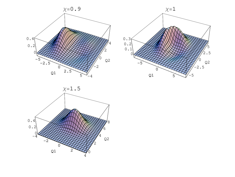
FIG. 1.: The numerical ground state wave functions at $\mu=2$ and $\chi=0.9$ (a) $\chi=1$ (b) and $\chi=1.5$ (c).

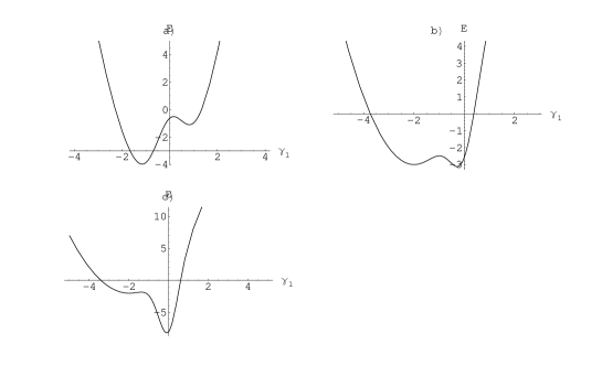
FIG. 2.: Shapes of the effective potential corresponding to the wave functions at Figs.1a, 1b and 1c, respectively.

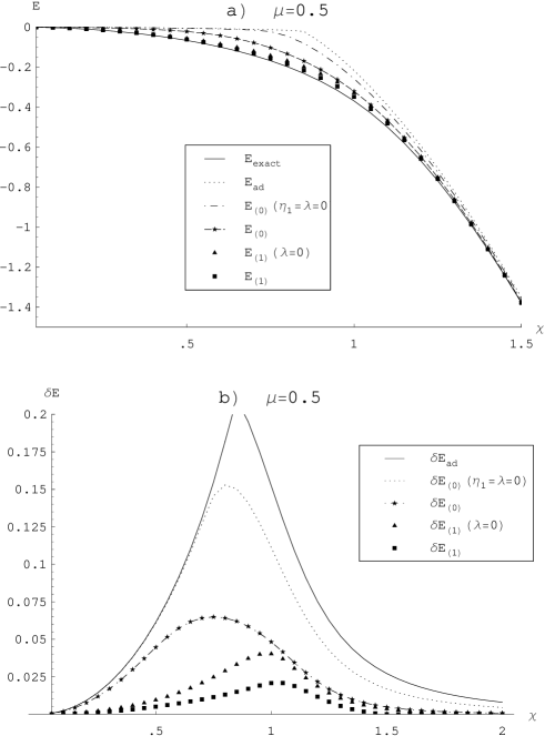
FIG. 3.: (a) The ground state energies (40) for $\mu=0.5$. The seltrapping dominated GS spans over $\chi<1$ and the tunneling dominated GS over $\chi>1$. The curves plotted represent cases (from below): numerical simulation GS, $E_{ex}$; ERA, $E_{1}$; ERA, $E_{1}(\lambda=0)$; SRA, $E_{0}$; SRA, $E_{0}(\eta_{1}=\lambda=0)$; adiabatic GS $E_{ad}$.
(b) Differences of the ground states from (a) and the exact numerical GS. ERA considerably improves the results for $\chi<1$. It also shifts the maximum of the differences to the point $\chi=1$.

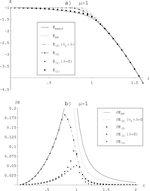
FIG. 4.: The same as in Fig. 3 for $\mu=1$. With increasing $\mu$, for $\chi<1$, the loss of efficiency of all VP except of $\eta_{2}$ is evident.

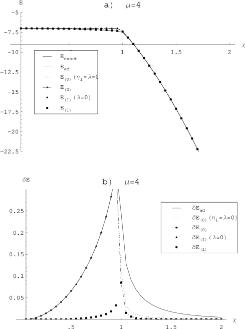
FIG. 5.: The same as in Fig. 3 and 4 for $\mu=4$.

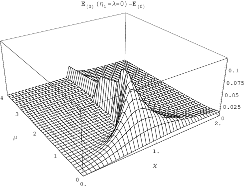
FIG. 6.: The difference of two GS: the GS without the reflection and correlation effects $E_{0}(\eta=0,\lambda=0)$ and the GS $E_{0}$ including these effects.

Figure Captions

Fig. 1. The numerical ground state wave functions at $\mu=2$ and $\chi=0.9$ (a) $\chi=1$ (b) and $\chi=1.5$ (c).

Fig. 2. Shapes of the effective potential corresponding to the wave functions at Figs.1a, 1b and 1c, respectively.

Fig. 3. (a) The ground state energies (40) for $\mu=0.5$. The seltrapping dominated GS spans over $\chi<1$ and the tunneling dominated GS over $\chi>1$. The curves plotted represent cases (from below): numerical simulation GS, $E_{ex}$; ERA, $E_{1}$; ERA, $E_{1}(\lambda=0)$; SRA, $E_{0}$; SRA, $E_{0}(\eta_{1}=\lambda=0)$; adiabatic GS $E_{ad}$.
(b) Differences of the ground states from (a) and the exact numerical GS. ERA considerably improves the results for $\chi<1$. It also shifts the maximum of the differences to the point $\chi=1$.

Fig. 4. The same as in Fig. 3 for $\mu=1$. With increasing $\mu$, for $\chi<1$, the loss of efficiency of all VP except of $\eta_{2}$ is evident.

Fig. 5. The same as in Fig. 3 and 4 for $\mu=4$.

Fig. 6. The difference of two GS: the GS without the reflection and correlation effects $E_{0}(\eta=0,\lambda=0)$ and the GS $E_{0}$ including these effects.

References

- [1] M. D. Kaplan and B. G. Vekhter, Cooperative phenomena in Jahn-Teller crystals. (Plenum, New York and London, 1995). Modern Inorganic Chemistry. Edited by V. P. Fackler.
- [2] O. Gunnarson, Phys. Rev. Lett. 74, 1875 (1995); O. Gunnarson, Rev. Mod. Phys. 69, 575 (1997).
- [3] K. A. Müller, J. Supercond. 12, 3 (1999).
- [4] M. C. M. O’Brien, and C. C. Chancey, Am. J. Phys. 61, 688 (1993).
- [5] J. L. Dunn, M. R. Eccles, Y. Liu, C. Bates, Phys. Rev. B, 65, 115107 (2002).
- [6] M. Wagner, and A. Köngeter, Phys. Rev. B 39, 4644 (1989).
- [7] H.B. Shore, and L.M. Sander, Phys. Rev. B7, 4537 (1973).
- [8] M. Sonnek, T. Frank, and M. Wagner, Phys. Rev. B 49, 15637 (1994).
- [9] H. Eiermann, and M. Wagner, J. Chem. Phys. 96, 4509 (1992).
- [10] H. Barentzen, Eur. Phys. J. B 24, 197 (2001).
- [11] E. Majerníková, J. Riedel and S. Shpyrko, Phys. Rev. B 65, 174305 (2002).
- [12] R.L. Fulton, and M. Gouterman, J. Chem. Phys. 35, 1059 (1961).
- [13] C. F. Lo, Phys. Rev. A 43, 5127 (1991).
- [14] P. Král, J. Mod. Opt. 37, 889 (1990).
- [15] B. L. Schumaker, Phys. Repts. 133, 317-408 (1986).