Edge dislocations in crystal structures considered as traveling waves of discrete models

Abstract

The static stress needed to depin a 2D edge dislocation, the lower dynamic stress needed to keep it moving, its velocity and displacement vector profile are calculated from first principles. We use a simplified discrete model whose far field distortion tensor decays algebraically with distance as in the usual elasticity. Dislocation depinning in the strongly overdamped case (including the effect of fluctuations) is analytically described. $N$ parallel edge dislocations whose average inter-dislocation distance divided by the Burgers vector of a single dislocation is $L\gg 1$ can depin a given one if $N=O(L)$. Then a limiting dislocation density can be defined and calculated in simple cases.

In many fields, genuinely microscopic phenomena affect macroscopic behavior in a way that is difficult to quantify precisely. Typical cases are the motions of dislocations nab67 ; hir82 , cracks fre90 , vortices in Josephson arrays zan95 or other defects subject to pinning due to the underlying crystal microstructure. Emerging behavior due to motion and interaction of defects might explain common but poorly understood phenomena such as friction ger01 . Macroscopic theories consider the continuum mechanics of these solids subject to forces due to the defects and additional equations for the densities of defects and properties of their motion ll7 . The latter are usually postulated by phenomenological considerations. An important problem is to derive a consistent macroscopic description taking into account the microstructure.

Here we tackle a simplified problem containing all the ingredients of the previous description: the pinning and motion of edge dislocations. Firstly, we study a two-dimensional (2D) discrete model kkl describing the damped displacement of atoms subject to the field generated by a 2D edge dislocation and a constant applied shear stress of strength $F$. If $|F|<F_{cs}$ ($F_{cs}$ is related to the static Peierls stress), the stable displacement field is stationary, whereas the dislocation core and its surrounding displacement field move if $|F|>F_{cs}$. A crucial observation is that there exists a stable uniformly moving dislocation with both core and far field advancing at the same constant velocity. This suggests that a moving edge dislocation is a traveling wave of the discrete model.

Our self-consistent calculation self based on this picture predicts the following magnitudes: (i) the critical static stress needed to depin a static dislocation, (ii) the dynamic stress $F_{cd}<F_{cs}$ below which a moving dislocation stops (in the strongly overdamped case, $F_{cd}=F_{cs}$), and (iii) the dislocation velocity as a function of applied stress. The latter information has to be taken from experiments in the standard treatment hul01 . Then a macroscopic quantity, the dislocation velocity, is obtained from analysis of a microscopic model.

Secondly, we consider a distribution of many parallel edge dislocations separated by macroscopic distances comprising many lattice periods. A dislocation cannot move under the influence of other dislocations far away unless the latter have finite density (there are $N$ such dislocations and the average distance between them is $L$ with $N=O(L)$ as $L\to\infty$). Under the influence of such a distribution, one dislocation may be pinned or move depending on the dislocation density. The latter is calculated at the critical stress in a simple configuration.

A simplified discrete model of edge dislocations. Consider an infinite three dimensional cubic lattice with symmetry axes $x,y,z$. We insert an extra half plane of atoms parallel to the plane $yz$. The border of this extra half plane is a line (parallel to the $z$ axis), which is called an edge dislocation in the crystal. The Burgers vector of the dislocation points in the $x$ direction and the plane $xz$ is the glide plane of the dislocation (see ll7 ). If we apply an external stress $\sigma$, the dislocation moves on its glide plane and in the direction of its Burgers vector in response to just one component of $\sigma$: the stress $\tau$ resolved on the glide plane in the glide direction hir82 ; ll7 . All the sections of the lattice by planes parallel to $xy$ look alike. Thus, we reduce the problem to a 2D lattice with an extra half line of atoms, see Fig. 22 of Ref. ll7, . Assuming that glide is only possible in the $x$-direction, the dynamics of an edge dislocation in a 2D lattice can be described by kkl :

$$m\,{d^{2}u_{i,j}\over dt^{2}} + {du_{i,j}\over dt}=u_{i+1,j}-2u_{i,j}+u_{i-1,j}$$ (1)

$$+ A\,[\sin(u_{i,j+1}-u_{i,j})+\sin(u_{i,j-1}-u_{i,j})].$$

The lattice is a collection of chains in the $x$ direction with elastic interaction between nearest neighbors within the same chain and sinusoidal interaction between chains. $u_{i,j}/(2\pi)$ is the dimensionless displacement of atom $(i,j)$ in the $x$ direction measured in units of the Burgers vector length $b$. $A>0$ measures the relative strengths of the nonlinear forces exerted by atoms on different planes $y=k$ (constant) and the linear forces exerted within any plane $y=k$. The dimensionless parameter $A$ also determines the width of the dislocation core ($\sim 1/\sqrt{A}$). Lastly, the time unit is the ratio between the friction coefficient and the spring constant in the $x$ direction. Then $m$ is the dimensionless ratio between the atomic mass times the spring coefficient and the square of the friction coefficient. In dislocation dynamics, an important case is that of overdamped dynamics, $m=0$ gro00 . Eq. (1) can be generalized to a vector model having a displacement vector $(u_{ij},v_{ij})$ and a continuum limit yielding the 2D Navier equations with cubic symmetry car03 . Such model has among its solutions edge dislocations with Burgers vectors in the $x$ or $y$ directions gliding in the direction thereof (which does not have to be assumed as in the present simple model). This model can also be solved using our methods at the expense of technical complications and high computational cost.

In this geometry, the far field of a static 2D edge dislocation is approximately given by the corresponding continuum elastic displacement $u_{ij}=u(x,y)$ with $x=\epsilon i$, $y=\epsilon j$ (where $\epsilon=b/L\ll 1$, $i$, $j$ are large and $L$ is the appropriate mesoscopic length). Then the stationary solutions of Eq. (1) satisfy the equations of anisotropic linear elasticity, $u_{xx}+Au_{yy}=u_{xx}+u_{YY}=0$, ($Y=y/\sqrt{A}$) far away from singularities and jumps kkl . The solution corresponding to the edge dislocation is the polar angle $\theta(x,Y)\in[0,2\pi)$, measured from the positive $x$ axis. Continuum approximations break down near the dislocation core, which should be described by the discrete model car97 . The advantadge of Eq. (1) compared to other 2D generalizations lom86 of the Frenkel-Kontorova model is that it yields the correct decay for strains and stresses: $r^{-1}$ as $r^{2}=x^{2}+Y^{2}\to\infty$, instead of exponential decay.

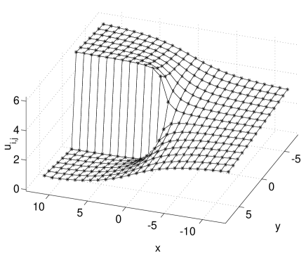
Figure 1: Displacement field profile for the stationary edge dislocation with $A=1$ and $N=50$.

Overdamped dynamics and static Peierls stress. We shall now study the structure of a static edge dislocation of Eq. (1), the critical stress needed to set it in motion and its subsequent speed. We solve numerically Eq. (1) with $m=0$ on a large lattice $|i|,|j|\leq N$ using Neumann boundary conditions (NBC) corresponding to applying a shear stress of strength $F$ in the $x$ direction. The (far field) continuum elastic displacement for a static 2D edge dislocation subject to such a shear stress is $\theta(x,y/\sqrt{A})+Fy$. Then the NBC are $u_{\pm(N+1),j}-u_{\pm N,j}=\pm[\theta^{A}_{\pm(N+1),j}-\theta^{A}_{\pm N,j}]$ and $u_{i,\pm(N+1)}-u_{i,\pm N}=\pm[\theta^{A}_{i,\pm(N+1)}-\theta^{A}_{i,\pm N}]\pm F$, where $\theta^{A}_{i,j}=\theta(i,j/\sqrt{A})$ with $\theta(0,0)=\pi/2$. If $F=0$ and the initial condition is the elastic far field $\theta^{A}_{i,j}$, the system relaxes to a stationary configuration $u_{i,j}$. The dislocation is expected to remain stationary for $F\neq 0$ unless $|F|$ is larger than a critical value $F_{cs}(A)$, related to the so called static Peierls stress nab67 ; hir82 . Nonlinear stability of the stationary edge dislocation for $|F|<F_{cs}$ was proven in Ref. car02, . To test this picture, we solve numerically Eq. (1) in a large lattice, using NBC and the static dislocation obtained for $F=0$ as initial data. For large times and $|F|$ small, the system relaxes to a steady configuration $u_{i,j}$ which provides the structure of the core, see Fig. 1. When $|F|$ is large enough, the dislocation is observed to glide in the $x$ direction: to the right if $F>0$, and to the left if $F<0$.

To calculate $F_{cs}$, we extend the depinning calculations of Ref. carPRL01, to 2D systems. We redefine $u_{i,j}=U_{i,j}+Fj$, insert $U_{i,j}=U_{i,j}(F,A)+v_{i,j}(t)$ in Eq. (1) with $m=0$ and expand the resulting equation in powers of $v_{i,j}$, about the stationary state $U_{i,j}(A,F)$ up to cubic terms. Subscripts in the resulting equation can be numbered with a single one starting from the point $i=j=-N$: $U_{i,j}=U_{k}$ and $v_{i,j}=v_{k}$, $k=i+(j+N)(2N+1)$ for $i,j=-N,\ldots,N$. The resulting equation can be written formally as $d{\bf v}/dt={\cal M}(F){\bf v}+{\cal B}({\bf v},{\bf v};F)$, where the vector ${\bf v}$ has components $v_{k}$. The linear stability of the stationary state $U_{k}(A,F)$ depends on the eigenvalues of the matrix ${\cal M}(F)$. These eigenvalues are all real negative for $|F|<F_{cs}$ whereas one of them vanishes at $|F|=F_{cs}$. This criterion allows us to numerically determine $F_{cs}$ as a function of $A$; see Fig. 2(a). Notice that the critical stress increases with $A$. Thus narrow core dislocations ($A$ large) are harder to move.

Dislocation velocity. Let us assume that $F>F_{cs}$ (the case $F<-F_{cs}$ is similar). Then $v_{ij}=(F-F_{c})j+\phi(t)r_{ij}$ (plus terms that decay exponentially fast in time). The procedure sketched in Refs. carPRL01, ; carPRE01, for discrete 1D systems yields the amplitude equation $d\phi/dt=\alpha+\beta\phi^{2}$. Here $\alpha={\bf l}\cdot{\cal N}(F_{cs})\,(F-F_{cs})/({\bf l}\cdot{\bf r})$, ${\cal N}_{ij}=A\,[\cos(U_{i,j+1}-U_{i,j}+F_{c})-\cos(U_{i,j}-U_{i,j-1}+F_{c})]$ and $\beta={\bf l}\cdot{\cal B}({\bf r},{\bf r};F_{cs})/({\bf l}\cdot{\bf r})$, ${\bf l}$ and ${\bf r}$ are the left and right eigenvectors of the matrix ${\cal M}(F_{cs})$ corresponding to its zero eigenvalue (its largest one). From the amplitude equation, the approximate dislocation velocity is carPRL01 : $c\sim\sqrt{\alpha\beta}/\pi=O(|F-F_{cs}|^{{1\over 2}})$. Numerically measured and theoretically predicted dislocation velocities are compared in Fig. 2(b). Calculations in lattices of different sizes yield similar results.

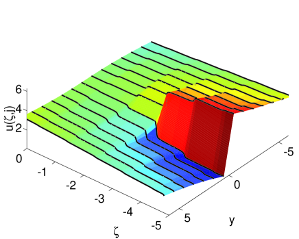
Figure 3: Wave front profiles, $u_{i,j}(t)=u(\zeta,j)$, $\zeta=i-ct$, $c>0$, near $F=F_{cs}$ for $A=3$, $m=0$ and $N=25$.

How do we calculate numerically the dislocation velocity? This is an important point for using the calculated dislocation velocity as a function of stress in mesoscopic theories and a few comments are in order. If we solve numerically Eq. (1) with static NBC for $|F|>F_{cs}$, the velocity of the dislocation increases as it moves towards the boundary. The dislocation accelerates because we are using the far field of a steady dislocation as boundary condition, instead of the (more sensible) far field of a moving dislocation. However, the latter is in principle unknown because we do not know the dislocation speed. We will assume nevertheless that the dislocation moves at constant speed $c$ once it starts moving, as it would in a stressed infinite system. Then the correct dislocation far field is $\theta(i-ct,j/\sqrt{A})+Fj$. With this far field in the NBC, Eq. (1) has traveling wave solutions $u_{i,j}(t)$ whose velocity can be calculated self-consistently. How? By an iterative procedure that adopts as initial trial velocity that of a dislocation subject to static NBC as it starts moving. Near threshold, step-like profiles are observed (see Fig. 3), that become smoother as $F$ increases. The profiles have been calculated by following the trajectories of points with the same value of $i$ and different values of $j$ for $F>F_{cs}(A)$, according to the formula $u_{i,j}(t)=u(\zeta,j)$, $\zeta=i-ct$. Notice that the wave front profiles are kinks for $j<0$ and antikinks for $j\geq 0$.

Influence of fluctuations. The original discrete model contains both damping and fluctuation terms kkl . Fluctuation terms are appreciable only near $F_{cs}$, and contribute an additive white noise term to the amplitude equation. Due to this term, there is a small probability for the dislocation to move even if $|F|<F_{cs}$ and $m=0$. The resulting average velocity can be estimated by observing that the potential of the corresponding Fokker-Planck equation is cubic and it has a small barrier of height proportional to $(F_{cs}-|F|)^{{3\over 2}}$. Then the exponentially small velocity of the dislocation under the critical stress is the reciprocal of the mean escape time from the barrier vankampen . Provided $(F_{cs}-|F|)\gg D$ (where $D$ measures the noise strength), we have $-\ln c\propto(F_{cs}-|F|)^{{3\over 2}}/D$.

Inertia and dynamic Peierls stress. Inertia changes the previous picture of dislocation motion in one important aspect: the dislocations keep moving for an interval of stresses below the static Peierls stress, $F_{cd}<|F|<F_{cs}$. On this stress interval, stable solutions representing static and moving dislocations coexist: to depin a static dislocation, we need $|F|>F_{cs}$. However if $|F|$ decreases below $F_{cs}$, a moving dislocation keeps moving until $|F|<F_{cd}$; see Fig. 2. Thus $F_{cd}$ represents the dynamic Peierls stress of the dislocation nab67 . Our theory therefore yields the static and the dynamic Peierls stresses and the velocity of a dislocation.

Interaction between edge dislocations. Let us assume that there are $N$ static edge dislocations at the points $(x_{n},y_{n})$ parallel to one dislocation at $(x_{0},y_{0})$, and that all dislocations are separated from each other by distances of order $L\gg 1$ (measured in units of the Burgers vector length, $b$). We want to analyze whether the collective influence of the $N$ distant dislocations can move that at $(x_{0},y_{0})$. This problem is similar to that of deriving a reduced dynamics for the centers of 2D vortices of Ginzburg-Landau equations subject to their mutual influence neu90 . In the case of dislocations, the existence of a pinning threshold implies that the reduced dynamics is that of a single dislocation subject to the mean field created by the others. We thus have a reduced field dynamics, not particle dynamics as in the case of the Ginzburg-Landau vortices.

Displacement vectors pose the problem of defining branch cuts in the continuum (elastic) limit, which leads us to consider instead the distortion tensor as a primary quantity ll7 . For our discrete system, the distortion tensor has nonzero components $w^{(1)}_{i,j}=u_{i+1,j}-u_{i,j}$ and $w^{(2)}_{i,j}=\sin(u_{i,j+1}-u_{i,j})$ that become $\epsilon\,(\partial u/\partial x)$ and $\epsilon\,(\partial u/\partial y)$, respectively, in the continuum limit $\epsilon=1/L\to 0$, $x-x_{0}=\epsilon i$, $y-y_{0}=\epsilon j$ finite. In the continuum limit, the distortion tensor of an edge dislocation centered at the origin has nonzero components $w^{(1)}=-\epsilon\sqrt{A}y/(Ax^{2}+y^{2})$ and $w^{(2)}=\epsilon\sqrt{A}x/(Ax^{2}+y^{2})$. If we have $N$ edge dislocations at $(x_{n},y_{n})$, $1\leq n\leq N$, far from one at $(x_{0},y_{0})$, the distortion tensor is sum of individual contributions. Then the far field distortion tensor seen by the dislocation at $(x_{0},y_{0})$ is:

$$w^{(1)}_{i,j}=-{\sqrt{A}j\over Ai^{2}+j^{2}}+F_{1},\quad\quad w^{(2)}_{i,j}={\sqrt{A}i\over Ai^{2}+j^{2}}+F_{2},$$ (2)

$$F_{1}=-\epsilon\sum_{n=1}^{N}{\sqrt{A}(y_{0}-y_{n})\over A(x_{0}-x_{n})^{2}+(y_{0}-y_{n})^{2}}+\ldots,$$ (3)

$$F_{2}=\epsilon\sum_{n=1}^{N}{\sqrt{A}(x_{0}-x_{n})\over A(x_{0}-x_{n})^{2}+(y_{0}-y_{n})^{2}}+\ldots.$$ (4)

The dislocation at $(x_{0},y_{0})$ moves if $F_{2}>F_{cs}(A)$. This cannot be achieved as $\epsilon\to 0$ unless $N=O(1/\epsilon)$. Then the sums in Eqs. (3) and (4) become integrals. We define a static dislocation density $\rho(x,y)$ as the limit of $N^{-1}\sum_{n=1}^{N}\delta(x-x_{n})\delta(y-y_{n})$ as $N\to\infty$. Then

$$F_{1}=-\alpha\int_{-\infty}^{\infty}\int_{-\infty}^{\infty}{\sqrt{A}(y_{0}-y)\rho(x,y)\over A(x_{0}-x)^{2}+(y_{0}-y)^{2}}\,dxdy,$$ (5)

$$F_{2}=\alpha\int_{-\infty}^{\infty}\int_{-\infty}^{\infty}{\sqrt{A}(x_{0}-x)\rho(x,y)\over A(x_{0}-x)^{2}+(y_{0}-y)^{2}}\,dxdy,$$ (6)

where $\alpha=\epsilon N$ is the ratio of the total Burgers vector to the mesoscopic length measuring average interdislocation distance. As an example, let us assume that $y_{0}=y_{n}=0$. Then $\rho=\rho(x)\delta(y)$ and $F_{1}=0$. Let us assume that the dislocations are constrained by two obstacles at $x_{0}=\pm l$ and subject to the same critical stress. Then the critical dislocation density is $\rho(x)=[1-(\sqrt{A}F_{cs}/\alpha)\,x]/[\pi\sqrt{l^{2}-x^{2}}]$, provided $\alpha>\sqrt{A}F_{cs}l$ (cf. ll7, , page 127).

In conclusion, edge dislocations can be characterized as traveling waves of discrete models. The dislocation far field moves at a constant velocity equal to that of the dislocation core. Static and dynamic Peierls stresses and the dislocation velocity as a function of applied stress can be found numerically (or analytically near critical stress in the overdamped case) and adopted as the basis of a mesoscopic theory gro00 . We have also shown that the interaction between distant edge dislocations can be described in terms of a continuous dislocation density. This field-theoretical reduced description greatly contrasts with the case of interacting point vortices, which is completely described by the particle dynamics of the vortex centers neu90 . Extension to fully vectorial models and to other types of dislocation should follow along similar lines.

We thank Joe Keller for helpful discussions. This work has been supported by the MCyT grant BFM2002-04127-C02, by the Third Regional Research Program of the Autonomous Region of Madrid (Strategic Groups Action), and by the European Union under grant HPRN-CT-2002-00282.

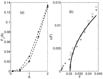
Figure 2: (a) Static (squares, $m=0$) and dynamic (asterisks, $m=0.5$) critical stresses $F_{cs}$ and $F_{cd}$ versus $A$. (b) Theoretical (solid line, $m=0$) and numerical (squares, $m=0$; asterisks, $m=0.5$) dislocation velocity vs. $F$ ($A=1$, $N=25$).

References

- (1) F.R.N. Nabarro, Theory of Crystal Dislocations (Oxford University Press, Oxford, 1967).
- (2) J.P. Hirth and J. Lothe, Theory of Dislocations (John Wiley and Sons, New York, 1982), 2nd ed.
- (3) L. B. Freund, Dynamic Fracture Mechanics (Cambridge University Press, Cambridge UK, 1990).
- (4) H.S.J. van der Zant, T.P. Orlando, S. Watanabe and S.H. Strogatz, Phys. Rev. Lett. 74, 174 (1995).
- (5) E. Gerde and M. Marder, Nature 413, 285 (2001). See also D.A. Kessler, Nature 413, 260 (2001).
- (6) L.D. Landau and E.M. Lifshitz, Theory of elasticity, 3rd ed. (Pergamon Press, London, 1986). Chapter 4.
- (7) A.I. Landau, A.S. Kovalev and A.D. Kondratyuk, Phys. stat. sol. (b), 179, 373 (1993); A.I. Landau, Phys. stat. sol. (b), 183, 407 (1994).
- (8) The far field of a dislocation is not spatially homogeneous and it should be rigidly and self-consistently displaced at the velocity of the dislocation core.
- (9) D. Hull and D.J. Bacon, Introduction to Dislocations, 4th ed. (Butterworth -Heinemann, Oxford UK, 2001).
- (10) I. Groma and B. Bakó, Phys. Rev. Lett. 84, 1487 (2000).
- (11) A. Carpio and L.L. Bonilla, unpublished.
- (12) A. Carpio, S. J. Chapman, S. D. Howison and J. R. Ockendon, Phil. Trans. R. Soc. Lond. A 355, 2013 (1997).
- (13) P.S. Lomdahl and D. J. Srolovitz, Phys. Rev. Lett. 57, 2702 (1986).
- (14) A. Carpio, Appl. Math. Lett. 15(4), 415 (2002).
- (15) A. Carpio and L.L. Bonilla, Phys. Rev. Lett. 86, 6034 (2001).
- (16) A. Carpio, L.L. Bonilla and G. Dell’Acqua, Phys. Rev. E 64, 036204 (2001).
- (17) N.G. van Kampen, Stochastic processes in Physics and Chemistry (North-Holland, Amsterdam 1981).
- (18) J.C. Neu, Physica D 43, 385, 407 and 421 (1990).