Connectivity Distribution of Spatial Networks

Abstract

We study spatial networks constructed by randomly placing nodes on a manifold and joining two nodes with an edge whenever their distance is less than a certain cutoff. We derive the general expression for the connectivity distribution of such networks as a functional of the distribution of the nodes. We show that for regular spatial densities, the corresponding spatial network has a connectivity distribution decreasing faster than an exponential. In contrast, we also show that scale-free networks with a power law decreasing connectivity distribution are obtained when a certain information measure of the node distribution (integral of higher powers of the distribution) diverges. We illustrate our results on a simple example for which we present simulation results. Finally, we speculate on the role played by the limiting case $P(k)\propto k^{-1}$ which appears empirically to be relevant to spatial networks of biological origin such as the ones constructed from gene expression data.

I Introduction

In contrast to abstract graphs, many real networks are embedded in a metric space: The interactions between the nodes depend on their spatial distance and usually take place between nearest neighbors. Examples of such networks are transportation and communication networks, friendship or contact networks[1, 2]. An especially important example is the Internet[3, 4], which is a set of routers linked by physical cables with different lengths. Several recent studies have investigated networks whose nodes are embedded in a metric space, and where the probability of connecting two nodes with an edge depends on their distance [1, 2, 4, 5, 6, 7, 8, 9, 10].

On the other hand, the concept of scale-free network has emerged in the last few years as a powerful unifying paradigm in the study of complex systems of natural, technological and social origin (see Refs. [11, 12]). It is therefore natural to investigate the possibility of embedding scale-free networks in space. In particular in Refs. [9, 10], the general problem of embedding a scale-free network of given connectivity distribution in a Euclidean lattice was studied.

In this paper we take a somewhat reversed point of view: Our starting point is a spatial distribution of points on a continuous manifold $M$. Such points are the nodes of a network built by joining two nodes whenever their distance is less than a certain cutoff. In the following we will call ‘spatial networks’ those obtained by this procedure (sometimes also termed as ‘ad hoc networks’ [2]). We study how the connectivity distribution depends on the distribution of the nodes on $M$. The fact that the nodes live in a continuous manifold rather than a lattice is important in generating scale-free networks since the number of neighbors that a node can have within a certain distance is not limited a priori by the lattice structure.

Spatial networks originating from a uniform distribution of the nodes were studied in Ref. [7], where it was shown that while the connectivity distribution takes the same Poisson form as in the Erdos-Renyi random networks (see eg. [13]), other important features, most notably the clustering coefficient, are radically different from the Erdos-Renyi case. The formation of giant clusters in such networks was studied in Ref. [7, 2].

A natural application of this class of networks is the study of epidemics propagation. While scale-free networks in which the connectivity does not depend on a pre-existing metric structure do not display an epidemic threshold [14], the situation changes when geographical closeness of two nodes influences their probability to be connected [9]. In our networks geographical closeness completely determines whether two nodes will be connected, so that we expect to find an epidemic threshold. Spatial networks appear to be a rather realistic model for epidemic propagation in animal or plant populations, where we do not expect any individual to have an interaction range very different from the average (as is the case for highly mobile human populations), while we do expect the population density to be non-uniform.

In addition, spatial networks of biological origin have also recently been constructed, especially from gene expression data obtained from micro-array experiments [15, 16, 17]. The connectivity distribution of such networks turns out to be a truncated power-law with the exponent of the power-law decay often close to unity. Interestingly, also networks constructed from gene expression data by a different rule[18], which does not satisfy our definition of a spatial network, display a similar connectivity distribution.

These facts motivated us to study how the connectivity distribution of a spatial network depends on the distribution of the nodes in space and under which conditions a scale-free network can be obtained, and finally whether an exponent close to unity plays any special role in this context.

II The connectivity distribution of a spatial network

A General Expression

The $N$ nodes of the network are supposed to be in a $D$-dimensional space and we will assume that they are distributed randomly in space with density $p(x)$. Given a node chosen at random, the probability that it is placed within a given domain of space $m$ is

$$\int_{m}dx\,p(x)$$ (1)

(we denote the integration measure by $dx$ independently of the dimension $D$). Once the nodes are distributed in this space, we have to construct the edges. We will use a simple cut-off rule: Given two nodes $i$ and $j$, located at $x_{i}$ and $x_{j}$ respectively, an edge will join them if

$$d(x_{i},x_{j})\leq R\ \ ,$$ (2)

where $d(x,y)$ is the distance between $x$ and $y$. Therefore, once the nodes have been distributed the network is completely determined by the choice of the cutoff $R$. This model follows strictly the rule used to construct networks based on gene expression data in Refs. [15, 16, 17], but more generally, it can be used to model the case where the interaction has a typical scale given by $R$.

Denoting by $B_{R}(x)$ the ball of radius $R$ centered in $x$

$$B_{R}(x)\equiv\{y\in M:d(x,y)<R\}\ \ ,$$ (3)

the probability that a given node is placed within $B_{R}(x)$ is

$$q_{R}(x)=\int_{B_{R}(x)}dx^{\prime}\,p(x^{\prime})\ \ .$$ (4)

If we consider a node located at $x$, the probability that it will have $k$ neighbors is then just the probability that $k$ additional nodes are located in the $B_{R}(x)$. The connectivity distribution for a node placed in $x$ is thus given by the binomial distribution

$$P(k;x,R)=\left(N-1\atop k\right)q_{R}(x)^{k}\,\left[1-q_{R}(x)\right]^{N-1-k}\ .$$ (5)

In the following, we will be concerned with the limit $N\to\infty$: In order to obtain a well defined connectivity distribution in this limit, one has to take the limit $R\to 0$, so as to ensure that the product

$$N\ V(R)$$ (6)

where $V(R)$ is the volume of the ball

$$V(R)=\int_{B_{R}(x)}dx\ \ ,$$ (7)

tends to a finite constant $\alpha$. This means that $R$ must scale as $N^{-D}$ as $N\to\infty$, and implies that the expected number of nodes found within the ball $B_{R}(x)$ remains finite in this limit:

$$N\,q_{R}(x)\to\alpha\ p(x)\ \ .$$ (8)

The constant $\alpha$ fixes the scale of the average connectivity $\langle k\rangle$ of the network. Indeed, from Eq.(11) derived below, it is easy to obtain the following relation between $\alpha$ and $\langle k\rangle$

$$\langle k\rangle=\alpha\int dx\,p^{2}(x)$$ (9)

Let us note that although the connectivity distribution is well-defined for any value $\alpha$, it has been shown in the case of a uniform density[7, 2] that the existence of a giant connected component implies a minimum value of $\alpha$ (or equivalently $\langle k\rangle$). We will not address this problem here but we can expect that for other densities there will be some similar conditions on $\alpha$ for the existence of a giant component.

In the limit $N\to\infty$, $R\to 0$, the connectivity distribution for a node located at $x$ is Poissonian and Eq.(5) becomes

$$P(k;x,\alpha)=\frac{1}{k!}\alpha^{k}p^{k}(x)e^{-\alpha p(x)}\ \ .$$ (10)

For the whole space, the connectivity distribution of the network is then obtained as the spatial average of the former expression and is

$$P(k;\alpha)=\frac{\alpha^{k}}{k!}\int dx\,p^{k+1}(x)e^{-\alpha p(x)}\ \ .$$ (11)

This formula solves the general problem of determining the connectivity distribution of a spatial network from the spatial distribution of the nodes. For a uniform distribution $p(x)$, we recover a Poissonian connectivity distribution as in Ref. [7]. However, Eq. (11) shows that other connectivity distributions can be obtained. In the following section we will determine under which condition a spatial node distribution generates a scale-free network instead.

B Scale-free spatial networks

Equation (11) allows us to determine the condition that must be satisfied by the node density $p(x)$ for the corresponding network to be scale-free. A network is scale-free if the moments $\langle k^{\nu}\rangle$ of its connectivity distribution diverge for $\nu$ larger than a certain $\nu_{\rm max}$. It is easy to compute the moments of the connectivity distribution of a spatial network from Eq. (11): For integer $\nu$ we have

$$\langle k^{\nu}\rangle_{\alpha} = \sum_{k}\alpha^{k}\frac{k^{\nu}}{k!}\int_{M}dx\,p^{k+1}(x)e^{-\alpha p(x)}$$ (13)

$$= \sum_{m=0}^{\nu}\sum_{k\geq m}\frac{\alpha^{k}}{k!}{\bf S}^{(m)}_{\nu}(k)_{m}\int dx\,p^{k+1}(x)e^{-\alpha p(x)}$$ (14)

$$= \sum_{m=0}^{\nu}{\bf S}^{(m)}_{\nu}\alpha^{m}\int dx\,p^{m+1}(x)\ \ ,$$ (16)

where $(k)_{m}=k(k-1)\dots(k-m+1)$ and ${\bf S}^{(m)}_{\nu}$ are the Stirling numbers of the second kind (see e.g. Ref. [19], p. 824), defined by

$$x^{\nu}=\sum_{m=0}^{\nu}{\bf S}^{(m)}_{\nu}x(x-1)\dots(x-m+1)\ \ .$$ (17)

It follows that $\langle k^{\nu}\rangle_{\alpha}$ exists if and only if the integrals

$$H_{a}\equiv\int dx\,p^{a+1}(x)$$ (18)

exist for all $a\leq\nu$. Conversely, the network is scale-free if there exists a $\nu_{\rm max}$ such that $H_{a}$ diverges for all $a\geq\nu_{\rm max}$. The integral Eq. (18) is a measure of the information contained in the probability distribution $p(x)$, and is simply related to the Renyi entropy [20]

$$R_{q}=\frac{1}{1-q}\log H_{q-1}\ \ .$$ (19)

C Classes of spatial networks

More generally, Eq. (11) allows us to determine the type of spatial network obtained for a given spatial node distribution. The networks can essentially be distinguished by the decay of the connectivity distribution for large connectivities[23]. For spatial networks, large connectivities are obtained in high density regions, namely maxima of $p(x)$. For the sake of simplicity, we will limit the discussion to the case of an isotropic distribution $p(x)=p(r)$ where $r$ is the modulus of $x$. We will also suppose that we have one density maximum located at $r=0$. We will then distinguish the following two cases:

• $p(0)=p_{0}$ is finite and decays sufficiently rapidly so that all the quantities $H_{a}$ are finite. This could be for instance the case for population density which is decreasing exponentially from the city center[21, 22]. In this case, an asymptotic evaluation of the integral in Eq. (11) shows that for large $k$ the connectivity distribution decays as

  $$P(k;\alpha)\sim\frac{(\alpha p_{0})^{k}}{k!k^{D}}\ \ .$$ (20)

  As expected, the low density fluctuations are reflected in the fast decay of the connectivity distribution and the corresponding spatial network will be of the ‘exponential’ type[23] (ie. the connectivity distribution decreases at least as fast as an exponential).

• $p(r\sim 0)\sim r^{-\beta}$ with $\beta<D$ (if $\beta>D$ a cut-off is needed to normalize $p(r)$ and we are in the first situation where the maximum of $p(r)$ is finite). In this case, the information measure $H_{a}$ will diverge for $a\geq\frac{D}{\beta}-1$ and the connectivity distribution is a power-law: Its large-$k$ behavior is given by (see section III)

  $$P(k;\alpha)\sim k^{-D/\beta}\ \ .$$ (21)

  The large density fluctuations allow here for the existence of nodes with very large connectivities and the corresponding network is scale-free.

Even if it might appear unlikely that spatial densities behave pathologically around some points, this is actually the case in many instances where the nodes live in an abstract space, with a distance defined by correlations. Such examples are obtained in the case of gene expression networks[15, 16, 17, 18] (or the stock market[24]) for which the distance is defined in terms of Pearson correlation coefficient between nodes. The spatial network has then a simple meaning: Two nodes are connected if their correlation is high enough. It has been observed that in this example, the connectivity distribution is a truncated power-law with exponent of order $1$[15, 16, 17].

D The dependence on the average connectivity

In this section we consider the dependence of the connectivity distribution (11) of a spatial network on the parameter $\alpha$ that, as discussed in Sec. 2, is a measure of the average connectivity. From Eq.(11) one immediately obtains the following equation governing the dependence of $P(k;\alpha)$ on $k$:

$$\frac{dP(k;\alpha)}{d\alpha}=\frac{1}{\alpha}\left[k\,P(k;\alpha)-(k+1)\,P(k+1;\alpha)\right]\ \ .$$ (22)

Note that while all spatial networks obey this equation, the converse is not true: One can easily construct connectivity distributions $P(k;\alpha)$ satisfying Eq. (22) that cannot be obtained from a spatial network.

Inspection of Eq. (22) shows that the limiting case $P(k)\propto k^{-1}$ corresponds to a fixed point, where the connectivity distribution does not depend on $\alpha$. This observation might be relevant in explaining the common appearance of scale-free networks with connectivity exponent $\sim 1$ constructed as spatial networks from gene expression data [15, 16, 17].

III A Simple Example of a Scale-free Spatial Network

In this section we discuss an explicit example of a one-dimensional distribution of nodes that generates a scale-free network. We calculate exactly the connectivity distribution in the limit of infinite number of nodes using Eq. (11). We also address the issue of finite-size effects and we compare the exact result for infinite size to numerical simulation for finite networks.

A Connectivity distribution for an infinite network

We consider the space to be the open interval $(0,1)$ and the node distribution to be

$$p(x)=(1-\beta)\ x^{-\beta},\ \ \ \ \beta<1\ \ .$$ (23)

The information measure $H_{a}$ is given by

$$H_{a}=(1-\beta)^{a+1}\int_{0}^{1}dx\,x^{-\beta(a+1)}\ \ ,$$ (24)

and diverges for

$$a\geq\frac{1}{\beta}-1\ \ .$$ (25)

Therefore we expect a scale-free network with $\langle k^{\nu}\rangle_{\alpha}$ divergent for $\nu\geq\frac{1}{\beta}-1$.

The connectivity distribution can be computed explicitly from Eq. (11) and is

$$P(k;\alpha) = \frac{\alpha^{k}}{k!}(1-\beta)^{k+1}\int_{0}^{1}dx\,x^{-\beta(k+1)}e^{-\alpha(1-\beta)\ x^{-\beta}}$$ (27)

$$= \frac{1}{\alpha\beta}\left[\alpha(1-\beta)\right]^{1/\beta}\frac{\Gamma\left[k+1-\frac{1}{\beta},\alpha(1-\beta)\right]}{\Gamma(k+1)}\ \ ,$$ (28)

where $\Gamma(x,a)$ is the incomplete Gamma function

$$\Gamma(x,a)=\int_{a}^{\infty}dt\,t^{x-1}e^{-t}\ \ .$$ (29)

Since for $z\to\infty$

$$\frac{\Gamma(z,a)}{\Gamma(z)}\to 1\ \ ,$$ (30)

we have for $k\to\infty$

$$P(k;\alpha) \sim \frac{1}{\alpha\beta}\left[\alpha(1-\beta)\right]^{1/\beta}\frac{\Gamma\left(k+1-\frac{1}{\beta}\right)}{\Gamma(k+1)}$$ (31)

$$\sim \frac{1}{\alpha\beta}\left[\alpha(1-\beta)\right]^{1/\beta}k^{-1/\beta}\ \ .$$ (32)

This result shows explicitly that scale-free networks with any value of the connectivity exponent down to 1 can indeed be obtained as a spatial networks, as it is observed in gene expression networks. Finally, we remark that the transition to a power-law behavior of the connectivity distribution (31) depends on $\alpha$ and $\beta$. Indeed, when the second argument $\alpha(1-\beta)$ of the incomplete gamma function tends to zero, we have a power-law behavior for $P(k;\alpha)$ even at small $k$, as can be seen from Fig. (1).

B Finite-size effects: Numerical results

Since real spatial networks contain a finite number of nodes and our analytical results were obtained in the limit of infinite networks, it is important to address the issue of finite size effects. In this section, we approach the problem from a numerical point of view by constructing finite spatial networks by Monte Carlo methods and comparing their connectivity distribution with the theoretical predictions.

The figure $1$ shows the result of such comparison for the one-dimensional spatial networks studied in the previous subsection, at $\beta=0.5$ and $\beta=0.9$, and $\alpha=5$. For a finite network, $\alpha$ is naturally defined as $2NR$, where $N$ is the number of nodes and $R$ is the distance cutoff used to define links. In each part of the figure, the connectivity distributions for $N=1000$ and $N=20000$ points are superimposed to the theoretical distribution given by Eq. (28). We can conclude that already for moderately sized networks the connectivity distribution is very close to the $N\to\infty$ behavior Eq. (28), thus indicating that our results provide a good approximation to the connectivity distribution of finite spatial networks.

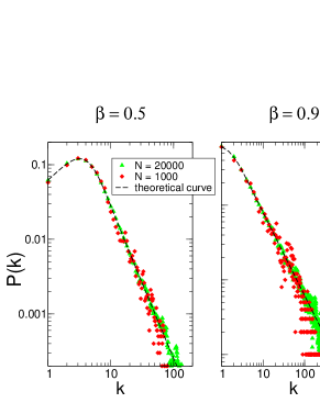
FIG. 1.: Monte Carlo simulation of the spatial networks constructed from the one-dimensional node distribution (23) compared to the $N\to\infty$ limit Eq.(28). The two figures refer respectively to $\beta=0.5$ (0.9) with $\alpha=5$, and show for each case the result for $N=1000$ and $N=20000$.

IV Discussion

We have presented a systematic analysis of the connectivity distribution of spatial networks constructed by joining nodes closer to each other than a cutoff distance, in the limit in which the number of nodes tends to infinity. The main results of our analysis can be summarized as follows. First, the connectivity distribution can be expressed as a functional of the spatial distribution of the nodes, Eq. (11). The moments of the connectivity distribution are related to a certain measure of information $H_{a}$ of the node distribution through Eq. (16). In particular, scale-free networks arise from this construction whenever the information measure $H_{a}$ diverges for some $a$ and we showed that scale-free networks with any exponent $\gamma>1$ can be constructed as spatial networks. Our results were obtained in the limit of infinite number $N$ of nodes but numerical results suggest that they provide an excellent approximation of real, finite spatial networks already for moderate $N$. Finally, the analysis of the dependence of the connectivity distribution $P(k;\alpha)$ on the connectivity scale $\alpha$ suggests that the limiting case $P(k)\propto k^{-1}$ corresponds to a fixed point, a fact that might be related to the empirical observation that several spatial networks constructed from gene expression data show a scale-free connectivity distribution with exponent close to 1.

Intuition suggests that spatial networks will be highly clustered and highly assortative. The clustering coefficient of spatial networks was studied in Ref. [7] for a uniform node distribution: However since the clustering coefficient is a local quantity and does not depend on the spatial density of nodes, the results of [7] should hold unchanged for all spatial networks, as long as the node distribution is isotropic in space. Moreover, spatial networks can be expected to display a high degree of assortativity, since high connectivity nodes are placed in high density regions and are therefore more likely to be connected to other high connectivity nodes. Indeed empirical spatial networks constructed from gene expression data show a high degree assortativity [16]. A closely related issue is the determination of the diameter of spatial networks. Due to the embedding in a metric space, we expect the diameter to grow as a power of the number of nodes, and therefore we do not expect spatial networks to belong to the small-world networks class.

Perhaps the most interesting open problem is to clarify the role of the limit case $P(k)\propto k^{-1}$, namely to classify the node distributions that flow to this fixed point in some limit. An example is given by Eq.(28) in the $\beta\to 1$ limit. $P(k)\propto k^{-1}$ implies that the measure of information $H_{a}$ diverges for all $a$, which in turn implies that the node distribution must become degenerate (that is its support must shrink to zero measure). However this is not a sufficient condition, since for example a Gaussian $p(x)$ in the limit of zero variance, while becoming degenerate, does not flow to $P(k)\propto k^{-1}$.

Acknowledgments: One of us (MB) thanks the department of physics-INFN in Torino for its warm hospitality during the time this work was completed.

REFERENCES

- [1] A. Helmy, e-print cs.NI/0207069.
- [2] G. Nemeth and G. Vattay, e-print cond-mat/0211325.
- [3] A. Lakhina, J.B. Byers, M. Crovella, and I. Matta, Technical report, online version available at: http//www.cs.bu.edu/techreports/pdf/2002-015-internet-geography.pdf
- [4] S.-H. Yook, H. Jeong, and A.-L. Barabasi, Proc. Natl. Acad. Sci. USA 99, 13382 (2000).
- [5] J. Jost and M. P. Joy, Phys. Rev. E 66, 036126 (2002).
- [6] M. Barthélemy, e-print cond-mat/0212086.
- [7] J. Dall and M. Christensen, Physical Review E 66, 016121 (2002).
- [8] P. Sen and S.S. Manna, e-print cond-mat/0301617.
- [9] C.P. Warren, L.M. Sander and I.M. Sokolov, e-print cond-mat/0207324.
- [10] D. ben-Avraham, A.F. Rozenfeld, R. Cohen and S. Havlin, e-print cond-mat/0301504.
- [11] R. Albert and A.-L. Barabasi, Rev. Mod. Phys. 74, 47 (2002).
- [12] S.N. Dorogovtsev and J.F.F. Mendes, Adv. in Phys. 51, 1079 (2002).
- [13] B. Bollobas, Random Graphs, Academic Press 1985.
- [14] R. Pastor-Satorras and A. Vespignani, Phys. Rev. Lett. 86, 3200 (2001).
- [15] P. Provero, e-print cond-mat/0207345.
- [16] C. Herrmann, F. Di Cunto, M. Pellegrino and P. Provero, submitted.
- [17] K. Rho, H. Jeong and B. Kahng e-print cond-mat/0301110.
- [18] H. Agrawal, Phys. Rev. Lett. 89 268702 (2002).
- [19] M. Abramowitz and I. A. Stegun (eds.), Handbook of mathematical functions, New York, Dover, 1964.
- [20] A. Renyi, Probability theory New York, Elsevier, 1980.
- [21] C. Clark, J. R. Stat. Soc. Ser. A 114, 490 (1951).
- [22] H.A. Makse et al, Phys. Rev. E 58, 7054 (1998).
- [23] L.A.N. Amaral, A. Scala, M. Barthélemy, and H.E. Stanley, Proc. Natl. Acad. Sci. USA 97, 11149 (2000).
- [24] R. N. Mantegna, Eur. Phys. J. B 11, 193 (1999).