Hole–defect chaos in the one–dimensional complex Ginzburg–Landau equation

Abstract

We study the spatiotemporally chaotic dynamics of holes and defects in the 1D complex Ginzburg–Landau equation (CGLE). We focus particularly on the self–disordering dynamics of holes and on the variation in defect profiles. By enforcing identical defect profiles and/or smooth plane wave backgrounds, we are able to sensitively probe the causes of the spatiotemporal chaos. We show that the coupling of the holes to a self–disordered background is the dominant mechanism. We analyze a lattice model for the 1D CGLE, incorporating this self–disordering. Despite its simplicity, we show that the model retains the essential spatiotemporally chaotic behavior of the full CGLE.

I Introduction

The formation of local structures and the occurrence of spatiotemporal chaos are among the most striking features of pattern forming systems. The complex Ginzburg–Landau equation (CGLE)

$$\partial_{t}A=A+(1+ic_{1})\partial_{x}^{2}A-(1-ic_{3})|A|^{2}A$$ (1)

provides a particularly rich example of these phenomena. The CGLE is the amplitude equation describing pattern formation near a Hopf bifurcation CH ; AK , and exhibits an extremely wide range of behaviors as a function of $c_{1}$ and $c_{3}$ CH ; AK ; chao1 ; phasediagram ; mvh ; maw ; mvhmh .

Defects and holes are local structures that play a crucial role in the intermediate regime between laminar states (small $c_{1}$, $c_{3}$) and hard chaos (large $c_{1}$, $c_{3}$). Isolated defects occur when $A$ goes through zero, where the complex phase $\psi:=\arg(A)$ is no longer defined. Homoclinic holes are localized propagating “phase twists”, which are linearly unstable. As illustrated in Fig. 1, holes and defects are intimately connected: defects can give rise to “holes”, which may then evolve to generate defects, from which further holes can be born, sometimes generating self–sustaining patterns. For more details see Refs. mvh ; mvhmh .

The aim of our paper is to understand and model the spatiotemporally chaotic hole–defect behavior of the 1D CGLE, built on the local interactions and dynamics of the holes and defects. Given the strength of the initial phase twist that generates a hole, and the wavenumber of the state into which it propagates, the hole lifetime $\tau$ turns out to be the key feature. Surprisingly, the initial phase twist and invaded state play very different roles. For hole–defect chaos, we will show that the defect profiles, which constitute the phase twist initial condition for the resulting daughter holes, show rather little scatter for fixed $c_{1}$ and $c_{3}$. Changes in $c_{1}$ and $c_{3}$, however, are encoded in changes in the defect profiles, and thus lead to changes in the typical lifetimes of the daughter holes. We then demonstrate that the chaos does not result from variations in defect profiles. It rather follows from the sensitivity of the holes to the states they invade, since the passage of each hole disorders the background wavenumber profile leading to disordered background states. It is the self–disordering action of the holes that is primarily responsible for the spatiotemporal chaos.

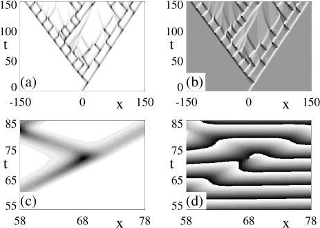
Figure 1: Illustration of the main phenomenology of hole–defect chaos (after Refs. phasediagram ; mvh ; mvhmh ). (a–b) Space–time grey–scale plots showing the invasion of a plane wave state by hole–defect chaos: (a) $|A|$ (dark: $A\!\approx\!0$) and (b) $q:=\partial_{x}\psi$ (light: $q\!>\!0$, grey: $q\!\approx\!0$, dark: $q\!<\!0$). The propagating objects are incoherent holes, which dynamically connect the defects (the black dots in (a)). Parameter values are $c_{1}\!=\!0.6,c_{3}\!=\!1.4$ , with an initial condition given by Eq. (2), with $\gamma\!=\!1,q_{ex}\!=\!-0.03$. The non–zero $q_{ex}$ breaks the left–right symmetry and results in the differing periods of the left and right moving edge holes. (c) Close–up of $|A|$ and (d) close–up of the complex phase $\psi$, showing in detail how a hole generates a phase defect that in turn generates two daughter holes.

With these insights, we can then construct a simplified lattice model for hole–defect chaos, which both reproduces the correct qualitative behavior as $c_{1}$ and $c_{3}$ are varied and which captures the correct mechanism (propagating, self–disordering holes). Our initial findings on this subject can be found in Ref. mvhmh , where we introduced the concept of self–disordering, and outlined a simplified lattice model. However in this paper, we investigate the subject in considerably greater depth, and, in particular, provide much more conclusive evidence for the correctnesss of the self–disordering hypothesis.

We now briefly summarize the structure of the paper. Topics discussed already in earlier work mvh ; mvhmh are dealt with rather briefly. We start in Section II by describing hole–defect dynamics on a local scale. In Section III, we then use this knowledge to investigate disordered hole–defect dynamics, and conclusively show that it is the coupling of the holes to a self–disordered background which is the dominant mechanism for spatiotemporal chaos. This concept is then illustrated by a minimal lattice model for hole–defect dynamics in Section IV, before we draw our conclusions in Section V.

II Hole–defect dynamics

We begin by studying the hole lifetime $\tau$ as a function of the initial conditions (Fig. 2). This study motivates the central question of this paper: how does $\tau$ depend on the initial conditions and on the external wavenumber, and which of these dependencies is most important for spatiotemporal chaos? We then study general properties of defect profiles, and demonstrate that in hole–defect chaos the profiles of defects show rather little scatter. We also show how the lifetimes of “daughter” holes born from a typical defect vary with $c_{1}$ and $c_{3}$. Taken together, the data presented here forms direct evidence for the heuristic picture of hole–defect dynamics developed in Refs. mvh ; mvhmh .

II.1 Incoherent homoclons

In full dynamic states of the CGLE, one does not observe the unstable coherent homoclinic holes unless one fine–tunes the initial conditions (see below). Instead evolving incoherent holes which either decay or start to grow towards defects occur mvh ; mvhmh . Let us consider the short–time evolution of an isolated incoherent hole propagating into a regular plane wave state. Holes can be seeded from initial conditions like mvhmh :

$$A=\exp(i[q_{ex}x+(\pi/2)\tanh(\gamma x)])~{}.$$ (2)

The two essential parameters $\gamma$ and $q_{ex}$ represent, respectively, the initial conditions from which the incoherent hole is born and the background wavenumber of the state into which the hole propagates. In this context, a single parameter $\gamma$ is sufficient to scan through different initial conditions, since the coherent holes have just one unstable mode mvh .

A detailed contour plot of the lifetime of an initial incoherent hole as a function of $\gamma$ and $q_{ex}$ is shown in Fig. 2. These results were obtained using a semi–implicit numerical integration of the CGLE, with space and time increments $dx=0.25$ and $dt=0.01$. As expected, three possibilities can arise for the time evolution of the initial peak: evolution towards a defect (upper right part of Fig. 2), decay (lower left part of Fig. 2), or evolution arbitrary close to a coherent homoclinic hole (the boundary between these two regions). These possibilities, together with an illustrative sketch of the phase space, are shown in the inset of Fig. 2. The rather simple and monotonic behavior of $\tau$ with $q_{ex}$ and $\gamma$ is somewhat of a surprise, and this reinforces our simple phase space picture; no other solutions seem to be relevant in this region of phase space.

Since homoclons are neither sinks nor sources, Fig. 2 can be interpreted as follows: for a right–moving homoclon an incoming wave with positive wavenumber tends to push the homoclon more quickly towards a defect; previously we have referred to this as “winding up” of the homoclon. Similarly, an incoming wave with negative wavenumber “winds down” a right–moving homoclon, possibly even preventing the formation of a defect mvh .

Figure 2: Contour plot showing the lifetime $\tau$ of an initial incoherent homoclon before a defect is generated. The initial condition is given by Eq.(2), and the lifetime is plotted as a function of $\gamma$ and $q_{ex}$. Note that the lifetime diverges as $q_{ex}$ or $\gamma$ are reduced. In the left–bottom corner of the diagram, the incoherent homoclon decays and no defects are formed. The inset shows a sketch of the phase space around the homoclon saddle (after Ref. mvhmh ), where the manifold $\Gamma$ represents the family of peaked initial conditions of the form (2).

II.2 Defects

We now study the defect profiles themselves in more detail. In Fig. 3a we show complex plane plots of $Re(a)$ vs. $Im(A)$ just before, close to, and just after a defect. As can be seen, there is no singular behavior whatsoever: the real and imaginary parts are smooth functions of $x$ and $t$, even at the time of defect formation. However, when transforming to polar coordinates, a singularity manifests itself at the defect, where $|A|\to 0$. This can also be seen from the $q$-profiles shown in Fig. 3b-d. In fact, it is straightforward to show that the maximum value of the local phase gradient $q_{m}$ diverges as $(\Delta t)^{-1}$ at a defect mvhmh , where $\Delta t$ is the time before defect nucleation (see Fig. 3b of Ref. mvhmh ) error .

In Fig. 3(e-g), we overlay complex plane plots of $A$ around $10^{3}$ defects obtained from numerical simulations of the CGLE in the chaotic regime. Surprisingly (see Fig. 3e), defect profiles of the interior chaotic states are dominated by a single profile in the hole–defect regime, similar to fixing $\gamma$ in Fig. 2. This provides a strong indication that hole–defect chaos does not come from scatter in the defect profiles. For large enough $c_{1}$ and $c_{3}$, where holes no longer play a role, and where hard defect chaos sets in maw , the profiles show a much larger scatter (Fig. 3(f,g)).

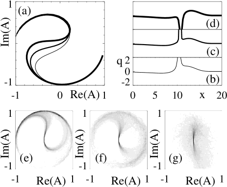
Figure 3: (a) Plots of the real and imaginary part of $A$ around a defect, just before (thin line), close to (medium line) and after (thick line) the defect has occurred; the time difference between successive profiles is $0.01$. Note that in this representation the dynamics looks completely smooth. (b-d) $q$-profiles for these three cases (identical vertical scale in each case); just before the defect occurs, a large positive spike develops in the profile, while after the defect this becomes a large negative spike. (e-g) Statistics of defects obtained by overlaying $10^{3}$ defect profiles of spatial extension (width) 20, centered around the defect position. An arbitrary phase factor has been divided out by requiring that $Re(\partial_{x}(A)|_{\rm{defect}})\!=\!0$. All data was collected in a system of size 500, after a transient of 500. The coefficients $c_{1}$ and $c_{3}$ are: (e) $0.6,1.4$, (f) $1.4,1.4$, (g) $3.0,3.0$.

II.3 Defect $\to$ holes

Suppose a hole has evolved to a defect; what dynamics occurs after this defect has formed? As Fig. 3(b-d) shows, defects generate a negative and positive phase–gradient peak in close proximity. The negative (positive) phase gradient peak generates a left (right) moving hole, and analogous to what we described in Fig. 2, the lifetimes of these holes depend on the initial peak and on $q_{ex}$. Hence the defect profile acts as an initial condition for its daughter holes, as can also clearly be seen in Fig. 1.

We now examine the fate of these daughter holes in the well–defined case where the initial defect is generated from the divergence of a right–moving, near–coherent homoclon in a $q_{ex}=0$ background state (see Fig. 4a). We then define $t_{1}$ and $t_{2}$ as the lifetimes of the resulting daughter holes. When a daughter hole does not grow out to form a defect, its lifetime diverges. In Fig. 4b we plot $t_{1}$ and $t_{2}$ for $c_{1}=0.6$ as a function of $c_{3}$. The initial hole that formed the first defect has a lifetime of at least $60$, and we have checked that a further increase of this time does not change $t_{1}$ and $t_{2}$ appreciably. When both $t_{1}$ and $t_{2}$ are infinite, no defect sustaining states can be formed, and the final state of the CGLE is in general a simple plane wave. When only $t_{1}$ is finite, isolated zigzag states are formed; such states have been discussed in Ref. mads , and we will see some examples below. When both $t_{1}$ and $t_{2}$ are finite, and of comparable value, more disordered states occur. We will later use this data on $t_{1}$ and $t_{2}$ to calibrate our minimal lattice model for spatiotemporal chaos.

Hence, we see that changes in $c_{1}$ and $c_{3}$ not only lead to changes in the defect profiles, but also modify the lifetimes of the resulting daughter holes. However, for fixed $c_{1}$ and $c_{3}$, we have seen that the defect profiles, which act as initial conditions for the daughter holes, show rather little scatter, at least in the hole–defect regime. In the next section, we will build on this knowledge to unravel the causes of hole–defect spatiotemporal chaos.

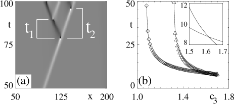
Figure 4: (a) Example of the divergence of a near–coherent right–moving hole, showing also the definition of times $t_{1}$ and $t_{2}$. (b) Times $t_{1}$ (diamonds) and $t_{2}$ (triangles) as a function of $c_{3}$ for $c_{1}=0.6$. The inset shows that the curves for $t_{1}$ and $t_{2}$ actually cross for sufficiently large $c_{3}$.

III Mechanism of hole–defect chaos

In this paper and in earlier work mvhmh , we have argued that the principal cause of the spatiotemporally chaotic behavior in the 1D CGLE is the movement of holes through a self–disordered background. Clearly, as we can see from Fig. 2, a disordered background wavenumber $q_{ex}$ will give rise to varying hole lifetimes and thus to disordered hole–defect dynamics. In this section, we explicitly demonstrate the correctness of this mechanism by modifying the CGLE dynamics in two ways:

Model (i): Fixed defect profile. Whenever a defect occurs, this defect is replaced by a standardized defect profile (obtained from an edge defect). Here the dynamics will be chaotic, showing the irrelevance of the scatter in defect profiles.

Model (ii): Background between holes $\rightarrow$ plane wave with $q\!=\!0$. At each timestep, the background between any two holes is replaced by a plane wave with wavenumber zero. Here no chaos will occur, illustrating the crucial importance of the self–disordered background.

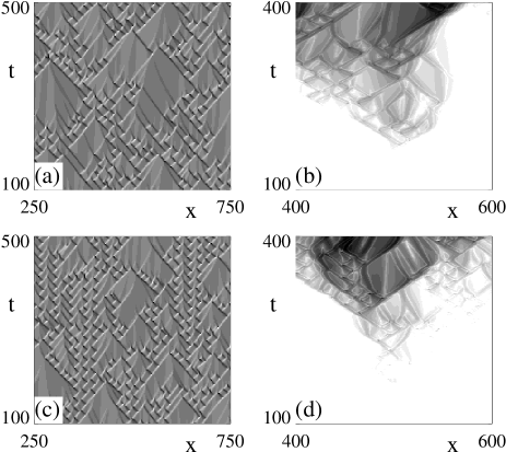
Figure 5: (a) Space–time plot of $q$ in the ordinary CGLE for $c_{1}=0.6,c_{3}=1.4$. (b) Log–greyscale plot of growth of perturbations. At $t=166.66,x=500$, one gridpoint was altered by $10^{-6}$. (c) Space–time plot of $q$ in model (i), the CGLE with fixed defect profiles. (d) Log–greyscale plot of growth of perturbations for the fixed defect model (i).

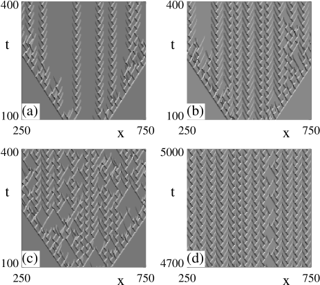
Figure 6: Dynamical states in model (ii), i.e., the CGLE where the background between holes is replaced by a $q=0$ plane wave. (a) For $c_{3}=1.4$ and $c_{1}=0.6$ only a few isolated zigzags occur. (b) When $c_{1}$ is increased to $0.7$, more zigzags occur, but there is no chaos. (c–d) For $c_{1}=0.8$, a disordered transient occurs (c) that eventually freezes into a quasiperiodic zigzag state without disorder (d).

In case (i), the size of the replaced defect profile was five centered around the defect; in case (ii) the background was defined to be all regions where $|A|>0.95$. Our results are substantially independent of the exact defect size or cutoff value. In both cases, it is crucial to ensure that no jumps in the phase occur at the edges of the replaced regions. This can be achieved by phase matching the replaced region (either defect profile or plane wave) at the left boundary, while the state to the right of the replaced region is multiplied by a phase factor to enforce phase–continuity at the right edge. We take open boundary conditions (i.e. $\partial_{x}A=0$) and only study the behavior far away from these boundaries.

In Fig. 5 we show an example of the dynamics and spreading of a localized perturbation for the full CGLE (Fig. 5a–b) and for the “fixed defect” model (i) (Fig. 5c–d), both for $c_{1}\!=\!0.6,c_{3}\!=\!1.4$. For both models, we took as an initial condition a defect rich state, which after a few timesteps shows the typical hole–defect dynamics. At $t\!\approx\!167$ we applied a local perturbation of strength $10^{-6}$ to the middle gridpoint (corresponding to $x\!=\!500$) and followed the evolution of both the perturbed and the unperturbed systems in order to follow the spreading of perturbations. For the full CGLE (Fig. 5a–b), the perturbation spreads along with the propagation of the holes. We note that the initial growth of the perturbation manifests itself in slight “shifts” of the spatial and temporal positions of the defects. In particular when two holes collide, a strong amplification of the perturbations is observed.

We can now compare this with the above fixed defect profile model (i) (Fig. 5c,d). Clearly, the replacement of the defects does not destroy the chaotic behavior of the system, as confirmed by the spreading of a localized perturbation (Fig. 5d), which propagates in a similar fashion to the full CGLE (Fig. 5b). This strongly indicates that variation in the defect profiles is not contributing in a major way to the spatiotemporally chaotic behavior of the full CGLE. We should also point out one subtlety here: due to the discretization of time, the times at which defect profiles are replaced are also discretized, and one may worry whether this destroys the chaotic properties of the model. However, we have performed simulations for a smaller timestep ($dt=0.001$) and found no qualitative difference. As we will see, this issue of discretization will play a more important role in the lattice model discussed in section IV.

Turning now to model (ii), where laminar regions of the CGLE are replaced by $q=0$ plane waves, we see that the disorder is destroyed. This is illustrated in Fig. 6, where we show examples of model (ii) dynamics for $c_{3}\!=\!1.4$ and $c_{1}\!=\!0.6,0.7,0.8$. Clearly chaos is suppressed for $c_{1}\!=\!0.6$ and 0.7 (Fig. 6a–b), with zigzag type patterns being especially dominant. For $c_{1}\!=\!0.8$ (Fig. 6c), the initial dynamics do appear disordered, but after a transient the system evolves to a regular zigzag state (Fig. 6d).

From the behavior of models (i) and (ii) we conclude that the self–disordered background is an essential ingredient for hole–defect chaos, while scatter in the defect profiles is not.

Figure 7: Grid model geometry showing the sites (dots) and hole propagation directions (arrows). The update rule is defined within a $2\times 2$ cell, mapping $(\phi_{l},\phi_{r})\rightarrow(\phi^{\prime}_{l},\phi^{\prime}_{r})$. “Active sites” where $|\phi|>\phi_{t}$ represent holes, while “inactive sites” where $|\phi|<\phi_{t}$ represent the diffusive background. When both sites are inactive the relevant dynamics is phase diffusion: $\phi^{\prime}_{r}\!=\!D\phi_{l}\!+\!(1\!-\!D)\phi_{r}$. The value of $D$ is fixed at $0.05$ and is not very important. When both sites are active, two holes collide and merge: $\phi^{\prime}_{r}\!=\!\phi^{\prime}_{l}\!=\!(\phi_{l}\!+\!\phi_{r})/2$. When one site is active but smaller than $\phi_{d}$, we implement the evolution noteA : $\phi^{\prime}_{r}\!=\phi_{l}+\!\lambda(\phi_{l}-\phi_{n}-g\phi_{r})$ (we assume here that we have a right moving hole, the case of a left moving hole follows by symmetry). Here $\lambda$ sets the time scale and can be taken small (fixed at $0.1$). When $\phi>\phi_{d}$ a defect occurs and two new holes, i.e., active sites, are generated; for details see text.

IV Lattice model

To further justify and test our picture of self–disordered dynamics, we will now combine the various hole–defect properties with the left–right symmetry and local phase conservation to form a minimal model of hole–defect dynamics. The model reproduces regular edge states, spatiotemporal chaos and can be calibrated to give the correct behavior as a function of $c_{1}$ and $c_{3}$. An earlier version of the model was presented in Ref. mvhmh . However, as will become clear, we have now modified and improved the model, and also for the first time made direct comparisons with the full CGLE.

From our earlier analysis (see also Ref. mvhmh ), we see that the following hole–defect properties must be incorporated in the model: (i) Incoherent holes propagate either left or right with essentially constant velocity. (ii) Their lifetime depends on $c_{1}$, $c_{3}$, and the wavenumber of the state into which they propagate. When the local phase gradient extremum diverges, a defect occurs. (iii) Each defect, in turn, acts as an initial condition for a pair of incoherent holes.

In our lattice model we discretize both space and time, and take a “staggered” type of update rule which is completely specified by the dynamics of a $2\times 2$ cell (see Fig. 7). We put a single variable $\phi$ on each site, where $\phi$ corresponds to the phase difference (the integral over the phase–gradient $q$) across a cell, divided by $2\pi$. Local phase conservation is implemented by $\phi^{\prime}_{l}\!+\!\phi^{\prime}_{r}\!=\!\phi_{l}\!+\!\phi_{r}$, where the primed (unprimed) variables refer to values after (before) an update. Holes are represented by active sites where $|\phi|>\phi_{t}$; here $\phi$ plays the role of the internal degree of freedom. Inactive sites are those with $|\phi|<\phi_{t}$, and they represent the background. The value of the cutoff $\phi_{t}$ is not very important as long as it is much smaller than the value of $\phi$ for coherent holes, and is here fixed at $0.15$. Without loss of generality we force holes with positive (negative) $\phi$ to propagate only from $\phi_{l}$ ($\phi_{r}$) to $\phi^{\prime}_{r}$ ($\phi^{\prime}_{l}$).

The details of the translation of these rules into the model can be found in the caption of Fig. 7 and in Ref. mvhmh , with one exception. A “defect” is formed when $\phi_{l}\!>\!\phi_{d}$. Here we have adopted two alternative schemes. In the simplest case (A) (studied before in Ref. mvhmh ), we take $\phi^{\prime}_{r}\!=\!\phi_{ad}$, and $\phi^{\prime}_{l}\!=\!\phi_{d}-1-\phi_{ad}$. Here we completely fix the new holes. The factor $-1$ reflects the change in the total winding number associated with the defects. Notice that the overall winding number does not change by exactly $-1$. This is because $\phi_{l}+\phi_{r}$ is usually slightly different from $\phi_{d}$. As we will discuss below, to avoid breaking this “phase conservation” we have also studied case (B), where we take $\phi^{\prime}_{r}\!=\!\phi_{ad}$, and $\phi^{\prime}_{l}\!=\!\phi_{l}+\phi_{r}-1-\phi_{ad}$. Here some (small) scatter in the defect profiles is allowed, but the change in the overall winding number is now strictly $-1$.

The model does contain a large number of parameters, $g$, $\phi_{n}$, $\phi_{d}$ and $\phi_{ad}$. We will first discuss the role of $g$ and the difference between the two defect rules (A) and (B).

In order for the model to reproduce the correct lifetime dependence of edge–holes in hole–defect states, the coupling of the holes to their background, $g$, should be taken negative (although its precise value is unimportant). For $g\!=\!0$ the hole lifetime $\tau$ becomes a constant, independent of the $\phi$ of the state into which the holes propagate, and moreover, the dynamical states are regular Sierpinsky gaskets (Fig. 8a). For $g\!<\!0$ both the appropriate $\tau$-divergence and disorder occur (Fig. 8b), illustrating the crucial importance of the coupling between the holes and the self–disordered background.

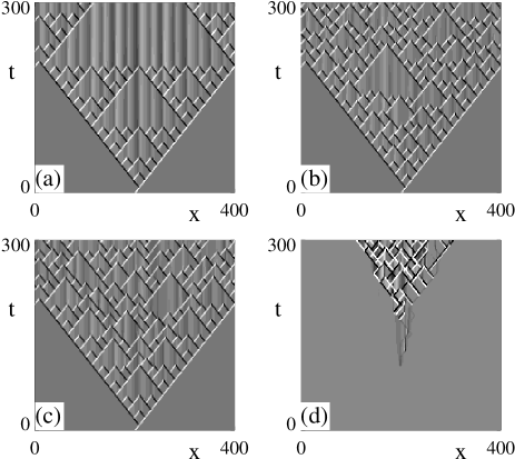
Figure 8: Illustration of the necessary ingredients for disorder and chaos in the grid model. In all cases, $\lambda=0.1,\phi_{ad}=0.75$, $\phi_{n}=0.59$, $\phi_{d}=1.01$ (this leads to $t_{1}=10,t_{2}=12$, which is the situation in the full CGLE for $c_{1}=0.6$ and $c_{3}=1.5$). (a) Without coupling to the background, $g=0$, the model with defect rule (A) leads to regular Sierpinsky gaskets. (b) When $g=-3$, the model generates disordered states, that are not strictly chaotic (see text). (c) When defect rule (B) is applied, also for $g=-3$, the dynamics is truly chaotic, as illustrated by the spreading of perturbations (d).

It turns out that the model with defect rule (A) is not strictly chaotic; sufficiently small perturbations do not always chaotically spread. However, with defect rule (B) implemented, infinitesimal perturbations do spread (see Fig. 8c,d). To understand this difference consider the fate of a tiny, localized perturbation. Holes will sweep past and be influenced by this perturbation, but since time is discrete, a sufficiently small perturbation will not lead to a change in the time at which a hole evolves to a defect. We have found that after a number of holes have passed over such a perturbation, it can actually be absorbed, so that no chaotic amplification occurs. It is therefore the combination of the discreteness of time and the fixed defect profiles which do not, strictly speaking, lead to chaos. By lowering $\lambda$, this problem is diminished, but this makes the model far less effective computationally. Alternatively, we have found that defect rule (B) also circumvents this problem; perturbations can now never be absorbed, due to the nature of the defect rule (B). In this case the defect profile is not entirely fixed, but its scatter is still rather small: for $\lambda=0.1$ a typical scatter is of the order of 5%, and this diminishes as $\lambda$ is decreased. Therefore we can conclude that, in the continuous time limit of the lattice model, the scatter of the defect profiles is not necessary to obtain chaos. In the remaining part of the paper, we will use model (B) only.

The self–disordering can be very clearly observed in the minimal model, since its update rules unambiguously specify which sites are “background” and which are ‘active”. Two snapshots of the evolution shown in Fig. 8c, are plotted in Fig. 9. These snapshots clearly demonstrate how, after sufficient time has passed, the “inactive” background between the holes has become completely disordered.

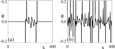
Figure 9: Illustration of the self–disordering in two snapshots of the field $\phi$ in our lattice model. Note that the scale is such that only the background is clearly visible; the peaks correspond to active, hole–like states. The data are taken from the runs shown in Fig. 8c, at (a) $t=60$ and (b) $t=300$.

The essential parameters determining the qualitative nature of the overall state are $\phi_{n}$, $\phi_{d}$ and $\phi_{ad}$. These parameters determine the amount of phase winding in the core of the coherent holes with $q_{ex}\!=\!0$ ($\phi_{n}$), and in the new holes generated by the defects ($\phi_{d}$, $\phi_{ad}$). When varying the CGLE coefficients, these parameters change too, leading to qualitatively different states. In particular, they determine the times $t_{1}$ and $t_{2}$ that we already studied for the full CGLE in section II.3. We found that when $\phi_{n}$ and $\phi_{ad}$ are both decreased, $t_{1}$ and $t_{2}$ roughly remain the same. We have therefore kept $\phi_{ad}=0.65$, and varied $\phi_{n}$ and $\phi_{d}$ to tune the values of $t_{1}$ and $t_{2}$. Notice that the symmetry (or asymmetry) of the defect profile depends on $\phi_{d}-1$; a value of $\phi_{d}<1$ typically promotes zigzag patterns. We have determined the appropriate values of $\phi_{n}$ and $\phi_{d}$ for three concrete cases, tabulated in Table I. Notice that the parameters for $c_{3}=1.5$ precisely correspond to those used in Fig. 8.

$c_{1}$	$c_{3}$	$t_{1}$	$t_{2}$	$\phi_{n}$	$\phi_{d}$
0.6	1.25	14	$\infty$	0.787	0.932
0.6	1.4	11	17	0.686	0.973
0.6	1.5	10	12	0.59	1.01

Table 1: Times $t_{1}$ and $t_{2}$ as obtained in the full CGLE, and appropriate coefficients $\phi_{n}$ and $\phi_{d}$ that reproduce these times in our grid model.

As can be seen in Fig. 10, the agreement between the simple model and the CGLE is satisfactory, although clearly the CGLE displays richer behavior. Note that in the full CGLE, small perturbations of the background wavenumber evolve in a non–trivial manner. For example, a nonzero average background wavenumber introduces a drift of the phase perturbations in the background between the holes torcinidrift . Since this phase dynamics is much slower than the hole–defect dynamics, we have chosen to ignore it in the grid model, and this accounts for the difference between Fig. 10a and Fig. 10b.

Finally, we emphasize that the grid model allows us to disentangle the mechanism of hole–defect chaos, by enabling us to completely control the behavior of defects and the coupling between holes and the laminar background. The grid model also has the advantage of being possibly the simplest model that captures the essence of the self–disordered hole-defect spatiotemporal chaos. We also emphasize that we have, for the first time, carried out a detailed comparison between the full CGLE and the grid model, both in our analysis of the spreading of perturbations and in the calibration of the grid model as a function of $c_{1}$ and $c_{3}$. Given the simplicity of the model, the agreement with the full CGLE is striking.

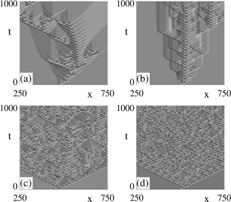
Figure 10: Comparison between the dynamics of the full CGLE (a,c) and our grid model (b,d), where $t_{1}$ and $t_{2}$ are matched according to Table I, with $c_{1}=0.6$, and (a-b) $c_{3}=1.25$ or (c-d) $c_{3}=1.4$.

V Conclusion

In conclusion, we have studied in depth the dynamics of local structures in the 1D CGLE. We have presented strong evidence that the origin of the chaotic behavior in the 1D CGLE lies in the self–disordering action of the holes, rather than in the scatter of the defect profiles. Using this insight, we have then developed a minimal lattice model for spatiotemporal chaos, which, despite its simplicity, reproduces the essential spatiotemporally chaotic phenomenology of the full CGLE.

How general are these results? We conjecture that there are two crucial properties needed for hole–defect type chaos: propagating saddle–like coherent structures (the holes) and a “conserved” field (the phase field). Of course, the phase is not strictly conserved here due to the occurrence of defects, but $(\int dx~{}\psi)~{}\mbox{mod }2\pi$ is a conserved quantity. It is this conservation that is weakly broken in our grid model for defect rule (A), but is preserved for defect rule (B). Only the latter is truly chaotic. The conservation is also the underlying reason why an evolving hole leaves an inhomogeneous and self–disordered trail behind. Without such a conserved field, there is no reason for “self–disordering” to occur, and the holes then typically will exhibit a fixed lifetime, leading to Sierpinsky gasket type patterns as is often the case in reaction–diffusion models rd . A related scenario appears to occur in the periodically forced CGLE chatepikovsky . Conserved fields of the type described here may be expected more generally for systems undergoing a Hopf bifurcation, and can therefore be expected to also occur in Ginzburg–Landau type equations including higher order terms, and also in experiments. We have argued in Ref. grr , that saddle–type structures like the homoclons here, may be much more general. This leads us to believe that the type of dynamics described here is not an artefact of the pure CGLE, but could be far more widespread.

Our work opens up the possibility for quantitative studies of hole–defect and homoclon dynamics, states which have recently been observed in various convection experiments garnier ; willem . We hope that our simple picture will advance these experimental studies of space–time chaos into the quantitative realm. Local dynamics of the type studied here, such as the dependence of lifetime on initial conditions grr , or measurements of quantities like the daughter hole lifetimes $t_{1}$ and $t_{2}$ should be accessible in experiment, thereby circumventing the difficulties normally associated with characterizing fully–developed chaotic states.

Finally, we mention another commonly observed type of spatiotemporal chaos occurring in systems when a periodic state undergoes a certain symmetry breaking bifurcation faivre . Mathematically, such systems may be described by a complex Ginzburg–Landau equation, coupled to a phase field. Such models are sometimes referred to as $A-\phi$ models aphi . Theoretically, the role of holes and defects has not yet been studied in great detail for these systems, but the main ingredients for hole–defect chaos of the type described here appear to be present. We hope that our work will encourage further studies in this area.

M.H. acknowledges support from Stichting FOM and from The Royal Society.

References

- (1) M. C. Cross and P. C. Hohenberg, Rev. Mod. Phys. 65, 851 (1993).
- (2) I. S. Aranson and L. Kramer, Rev. Mod. Phys. 74, 99 (2002).
- (3) B. I. Shraiman, A. Pumir, W. van Saarloos, P. C. Hohenberg, H. Chaté and M. Holen, Physica D 57, 241 (1992).
- (4) H. Chaté, Nonlinearity 7, 185 (1994).
- (5) M. van Hecke, Phys. Rev. Lett. 80, 1896 (1998).
- (6) L. Brusch et al., Phys. Rev. Lett. 85, 86 (2000).
- (7) M. van Hecke and M. Howard, Phys. Rev. Lett. 86, 2018 (2001).
- (8) Note that the scale of the axis in Fig. 3b of Ref. mvhmh should be a factor of smaller than labeled.
- (9) M. Ipsen and M. van Hecke, Physica D 160, 103 (2001).
- (10) This equation is a simplified version of the quadratic evolution equation for the holes introduced in Ref. mvhmh . This quadratic equation describes the finite time divergence of the local phase gradient extremum as a hole evolves towards a defect. However, even though diverges at a defect, its local integral does not. Hence, the finite time divergence of the local phase gradient maximum that signals a defect, can be replaced by a cutoff for mvhmh .
- (11) T. Kawahara, Phys. Rev. Lett. 51, 381 (1983); A. Torcini, Phys. Rev. Lett. 77, 1047 (1996).
- (12) W. N. Reynolds et al., Phys. Rev. Lett. 72, 2797 (1994); M. Zimmermann et al., Physica D 110, 92 (1997); A. Doelman et al., Nonlinearity 10, 523 (1997); Y. Hayase and T. Ohta, Phys. Rev. Lett. 81, 1726 (1998); Y. Nishiura and D. Ueyama, Physica D 130, 73 (1999).
- (13) H. Chaté, A. Pikovsky and O. Rudzick, Physica D 131, 17 (1999).
- (14) M. van Hecke, Physica D 174, 134 (2003).
- (15) N. Garnier, A. Chiffaudel, F. Daviaud and A. Prigent, Physica D 174, 1 (2003); N. Garnier, A. Chiffaudel and F. Daviaud, Physica D 174, 30 (2003).
- (16) L. Pastur, M. T. Westra and W. van de Water, Physica D 174, 71 (2003); L. Pastur, M. T. Westra, D. Snouck, W. van de Water, M. van Hecke, C. Storm and W. van Saarloos, Phys. Rev. E 67, 036305 (2003).
- (17) S. Akamatsu and G. Faivre, Phys. Rev. E, 58, 3302 (1998); P. Brunet, J. M. Flesselles and L. Limat, Europhys. Lett. 56, 221 (2001).
- (18) P. Coullet and G. Iooss, Phys. Rev. Lett. 64 866 (1990).