Quantum interference in nested $d$-wave superconductors: a real-space perspective

Abstract

We study the local density of states around potential scatterers in $d$-wave superconductors, and show that quantum interference between impurity states is not negligible for experimentally relevant impurity concentrations. The two impurity model is used as a paradigm to understand these effects analytically and in interpreting numerical solutions of the Bogoliubov-de Gennes equations on fully disordered systems. We focus primarily on the globally particle-hole symmetric model which has been the subject of considerable controversy, and give evidence that a zero-energy delta function exists in the DOS. The anomalous spectral weight at zero energy is seen to arise from resonant impurity states belonging to a particular sublattice, exactly as in the 2-impurity version of this model. We discuss the implications of these findings for realistic models of the cuprates.

I Introduction

Improvements in high-resolution scanning tunneling microscopy (STM) applied to superconductors yazdani ; davisnative ; davisZn ; cren ; davisinhom1 ; davisinhom2 ; Kapitulnik1 ; Kapitulnik2 ; Hoffman1 have raised the prospect of obtaining completely new kinds of local information about the cuprate materials, which may bear on the origins of the high-temperature superconductivity itself. Interpretation of these experiments is understood to be a delicate matter, but until now has been undertaken at only the naivest levels for want of theoretical tools for studying the local properties of strongly correlated systems. As an example, one may consider the discovery of subgap impurity resonances at low temperatures in the superconducting state by STMyazdani ; davisnative ; davisZn : while comparisons of STM data on disordered BSCCO-2212 with the simplest calculations of a single potential scatterer in a $d$-wave superconductorscalapino ; Balatsky ; otherlocaldos were understood early on to be only approximately successful, it was immediately proposedvojta ; Zhufilter ; martinbalatsky that more complicated (but still local) 1-impurity Hamiltonians or STM tunneling matrix elements could resolve the discrepancies. Only recently has it been pointed out that quantum interference of impurity states might make it difficult to observe true 1-impurity properties at allMorr ; zhutwoimpurity . In order for STM to fulfill its promise, it is vital to understand the extent to which long-range quantum interference due to disorder influences ostensibly local properties.

The problem of low-energy $d$-wave quasiparticle excitations in the cuprates in the presence of disorder is still unsolved (for a review, see HAreview ). Traditionally, it has been assumed that the appropriate disorder potential is some random distribution of short-range (and possibly magnetic) scatterers. More recently, there has been a gradual recognition that nanoscale spatial inhomogeneities are frequently, and possibly always, present in HTSC. cren ; davisinhom1 ; Kapitulnik1 ; Hoffman1 In most current theories, disorder is treated in the so-called self-consistent $T$-matrix approximation (SCTMA) which makes predictions for macroscopic properties of disordered systems. The SCTMA predicts, for example, a constant residual Fermi level density of quasiparticle states $\rho(0)$, which should dominate the low-energy transport over an energy range $\gamma$ referred to as the “impurity bandwidth”, in analogy to similar phenomena in semiconductors. Transport and thermodynamic measurements on the cuprates appear to support qualitatively the predictions of this simple approach though there are lingering quantititative differences which require resolutionHussey . The SCTMA neglects “crossing diagrams” corresponding to self-retracing scattering paths in real space, and attempts to go beyond the SCTMA have produced a variety of strongly model-dependent results for the density of states (DOS), many of which do not support the idea of an impurity band (constant DOS energy range) at all. In these nonperturbative calculations, the asymptotic limit $\rho(0)$ may vanishtsvelik ; fisher ; atkinsonops , saturate at a finite valueziegler or divergepepinlee ; mudry ; otherdivergence depending on the symmetry of the Hamiltonianatkinsondetails ; yashenkin . We also note a recent semi-classical treatment of extended impurities suggesting a divergent density of states at the Fermi levelgoldbart .

In this paper, we perform simple, exact calculations of the interference of two impurities in a $d$-wave superconductor, and compare to numerical calculations for many-impurity systems, in order to investigate the formation of the impurity band. Spatial fluctuations in the local DOS, which become quite complicated as a result of interference between impurities, contain information about both the SCTMA impurity band and about the quantum interference processes responsible for weak localization physics. For purposes of this paper, it is useful to make a distinction between quantum interference associated with weak localization and local interference patterns seen, for example, in STM experiments. We restrict ourselves in this initial work to a half-filled, tight-binding band with infinite potential scatterers. This model has nesting symmetries which distinguish it from the cuprate superconductors, but is nevertheless interesting from two points of view, that transparent analytical results for some properties can be obtained, and that the character of the divergence of the density of states near half-filling is controversialHAreview . The two-impurity problem is the simplest problem which includes the interference processes which lead to the formation of the impurity band, as well as processes which lead to weak localization.

Early work on the two-impurity problem in a $d$-wave superconductor was numerical in nature and focussed on the local density of states (LDOS), exhibiting unusual local interference patterns which depended on the orientation of the vector $\bf R$ separating the two impurities.Miyake More recently, the relation to impurity band formation was discussedmicheluchi and predictions were made for STM experimentsMorr ; zhutwoimpurity , assuming that ”sufficiently isolated” two impurity configurations could be identified. In reference zhutwoimpurity , the bound state wavefunctions of the two-impurity system were identified and classified. By analogy with the molecule problem in quantum mechanics, one expects that the single-impurity resonance energies split as the impurities are brought together, and that the wavefunctions are formed from symmetric and antisymmetric combinations of the isolated impurity wavefunctions. In fact, because of the particle-hole and fourfold rotational symmetries of the superconducting state, the situation is more complicated, with the effective overlap depending on $\bf R$ . Indeed, it has been shown that for many pair configurations, the density of states does not consist of four well-defined resonancesMorr ; zhutwoimpurity .

The interference between impurities persists up to large impurity separations. In Ref. zhutwoimpurity it was noted that two impurities with ${\bf R}\parallel(110)$ could cause splittings comparable to the original resonance energy for $R$ of many tens of lattice spacings. The spatial LDOS maps are therefore very different from superposed single-impurity maps, and one may ask the question whether this distinction persists in the case of many impurities. That is, is it to be expected at experimental impurity concentrations that a resonance found by STM really corresponds to an isolated impurity whose LDOS is predictable within a simple 1-impurity modelzhutwoimpurity ? Alternatively, are interference effects omnipresent, destroying expected 1-impurity resonances and leading to new, long range LDOS patterns which require a many-impurity interpretation? If the latter scenario is realized, how can it be that STM experiments seem to see such similar spectra on or near impurities embedded in very different local disorder environments? We resolve these questions below by arguing that in the generic case the individual many-impurity eigenstates are highly distorted from mere superpositions of 1-impurity LDOS patterns, but that STM measurements tend to average over many such eigenstates, cancelling some of the long-range effects of interference. Exceptions are very low energy states of the nested d-wave superconductor, which experience symmetry-driven level repulsion effects which prevent such cancellations. These considerations lead to a picture where, with the exception of the zero energy states, the local impurity resonances appear homogeneously broadened to any probe which averages over a macroscopic energy window. This result has important consequences for the interpretation of STM spectra. It means that, while the position of a peak and the crude local LDOS pattern at an energy near the peak may indeed qualitatively reflect one-impurity properties, e.g. the strength of the 1-impurity potential $V_{0}$, the widths of spectral features measured at any site will reflect the impurity bandwidth $\gamma$ characteristic of the disordered system as a whole.

Figure 1: Schematic figure of the many-impurity DOS (a) in the unitary limit of the half-filled band and (b) in the unitary limit of a generic band. The plateau in the impurity band is characterized by a nearly constant density of states $\rho_{0}$. The zero-energy suppression in (b) is discussed in Refs. fisher ; atkinsondetails

The second goal of this paper is to investigate the divergence in the total density of states in the completely nested model from a local point of view, applying what we can learn about the 2-impurity system. In contrast to the prediction of a residual $\rho(0)$ by the SCTMA, Pépin and Lee (PL)pepinlee found that, for an infinite scattering potential, the disorder-averaged density of states should diverge at the Fermi level (taken to be the zero of energy here) as $\rho(\omega)\approx n_{i}/\omega\log^{2}\omega$ where $n_{i}$ is the density of impurities. The schematic picture of the total DOS in this case is exhibited in Fig. 1a), to be contrasted with the more generic case expected in the absence of the nesting symmetry (1b). One surprising aspect of the PL result for the $N$-impurity $T$-matrix is that it is essentially $n_{i}$ times the single-impurity result. Upon closer inspection, however, their result is not directly tied to the one-impurity resonance at the Fermi-level, but is the result of interference between distant impurities. Numerical calculations showed that the divergence arises because of a global particle-hole symmetryatkinsondetails which is particular to the tight-binding model at half-filling. It was later shown that this nesting leads to a novel diffusion modeyashenkin producing a positive logarithmic correction to the DOS. This general structure of the divergence has also been found by Mudry and Chamonmudry and numerical calculationsZhu seem to confirm it, although in both cases the strength of the divergence could not be verified. The situation is not settled, however, and other recent field-theoretical approachesotherdivergence find a different form for the divergence which is reminiscent of the half-filled normal metal. The investigations of the 2– and many-impurity problem presented here paint yet a different picture. While (for reasons discussed in the text) it is difficult to rule out the existence of a continuous divergent contribution, we argue that the strong divergence in $\rho(E\rightarrow 0)$ seen in previous numerical work is actually indicative of a delta-function divergence at the Fermi level. In the final stages of writing this work, we became aware of a recent conserving weak-localization calculationyang which comes to the same conclusion.

The paper is organized as follows: in section II.1 we derive expressions for the Green’s functions $\hat{G}({\bf r},\omega)$ needed to evaluate the two-impurity T-matrix. Asymptotic expressions for large ${\bf r}$ have been found previouslyjoynt ; BalatskySalkola ; pepinlee and our results, valid for small $\omega$, are complementary. In section II.2 we specialize to the fully nested strong scattering model, evaluate the density of states for different impurity configurations, and show that there are three different classes of impurity-pair orientation. For two of these classes, the DOS diverges as $\omega\rightarrow 0$, while the DOS vanishes for the third. In all three cases, interference between impurities is substantial as in Ref. pepinlee , but ultimately the observed divergences arise from the local rather than nonlocal correlations. In section III we establish a connection between the zero-energy LDOS of the fully nested disordered system and the zero-energy DOS of the one- and two-impurity problems. For the fully nested model, we find that, in a given configuration, only impurities on a given sublattice contribute to the resonant weight at zero energy. The impurities in this class form a network with spatial separations equivalent to the resonant configurations in the 2-impurity case, and numerical scaling of the total spatially integrated DOS is shown to be consistent with $\rho(\omega)\sim\delta(\omega)$.

In section IV, we summarize our conclusions and discuss the less symmetric situation found in the cuprates. We argue that, because the STM averages over many multi-impurity eigenstates, the LDOS indeed appears to represent a set of nearly isolated impurity states with spectral features which are similar from impurity to impurity. On the other hand, we expect the width of these local states in energy to be typically the impurity bandwidth arising from the full disordered system.

II Two impurities in a half-filled band

II.1 Green’s functions

The BCS Hamiltonian for a pure $d$-wave singlet superconductor in a tight-binding band can be written as:

$$H_{0} = \sum_{{\bf k}}\Phi_{{{\bf k}}}^{\dagger}[(\epsilon_{{\bf k}}-\mu)\hat{\tau}_{3}+\Delta_{k}\hat{\tau}_{1}]\Phi_{{\bf k}},$$ (1a)

$$\epsilon_{\bf k} = -2t(\cos k_{x}+\cos k_{y}),$$ (1b)

$$\Delta_{\bf k} = \Delta_{0}(\cos k_{x}-\cos k_{y}),$$ (1c)

where $\Phi_{{\bf k}}=(c_{{\bf k}\downarrow}c^{\dagger}_{-{\bf k}\uparrow})$ is a Nambu spinor, and $\hat{\tau}_{i}$ are the Pauli matrices. Energies are measured relative to the center of the band, so a chemical potential of $\mu=0$ corresponds to half-filling. The associated Green’s function is, in real space, a function of the relative coordinate ${\bf r}=(m,n)$, where ${\bf r}$ is measured in units of the lattice constant and $m$ and $n$ are integers:

$$\hat{G}^{0}({\bf r},\omega) = \sum_{\bf k}e^{i{\bf k}\cdot{\bf r}}\hat{G}^{0}({\bf k},\omega),$$ (2)

$$= \sum_{{\bf k}}\cos(k_{x}m)\cos(k_{y}n)$$

$$\times\frac{\omega\hat{\tau}_{0}+(\epsilon_{k}-\mu)\hat{\tau}_{3}+\Delta_{\bf k}\hat{\tau}_{1}}{\omega^{2}-E_{\bf k}^{2}},$$

where $E_{\bf k}=\sqrt{\epsilon_{\bf k}^{2}+\Delta_{\bf k}^{2}}$ denote quasiparticle energies, $\hat{~{}}$ denotes a matrix in Nambu space and the superscript denotes the bare Green’s function. Frequently, it is convenient to make the decomposition in terms of Nambu spinors

$$\hat{G}^{0}({\bf r},\omega)=\sum_{j=0}^{3}G^{0}_{j}({\bf r},\omega)\hat{\tau}_{j}.$$

An ensemble of $N$ short-range scattering potentials at a set of sites ${\bf R}_{i}$ introduce a perturbation

$$H_{imp} = V_{0}\sum_{i=1}^{N}\Phi_{{\bf R}_{i}}^{\dagger}\hat{\tau}_{3}\Phi_{{\bf R}_{i}}$$

where $V_{0}$ is the strength of the impurity potential. Formally, there is an exact solution for the disordered Green function in terms of the $2N\times 2N$ many-impurity T-matrix:

$$\hat{G}({\bf r},{\bf r}^{\prime},\omega) = \hat{G}^{0}({\bf r}-{\bf r}^{\prime},\omega)$$

$$+\sum_{i,j}\hat{G}^{0}({\bf r}-{\bf R}_{i},\omega)\hat{T}_{ij}(\omega)\hat{G}^{0}({\bf R}_{j}-{\bf r},\omega)$$

with $i,j$ the position indices of the impurity sites, and

$${\bf\hat{T}}=[{\bf 1}\otimes\hat{\tau}_{0}-\hat{\tau}_{3}V_{0}{\bf\hat{G}^{0}}(\omega)]^{-1}{\bf 1}\otimes\hat{\tau}_{3}V_{0},$$

where the boldface indicates a matrix in spatial indices in the subspace of impurity sites (ie. ${\bf\hat{G}^{0}}_{ij}(\omega)=\hat{G}^{0}({\bf R}_{i}-{\bf R}_{j},\omega)$) and the inverse is a matrix inverse. In the limit of a single impurity, the T-matrix simplifies to $\hat{T}(\omega)=[V_{0}^{-1}\hat{\tau}_{3}-\hat{G}^{0}(0,\omega)]^{-1}$, with $\hat{G}^{0}(0,\omega)\equiv\hat{G}^{0}({\bf r}=0,\omega)$. This limit has been studied extensively.

In this work, we are particularly interested in the two-impurity T-matrix with one impurity at the origin (for simplicity) and the other a displacement ${\bf R}=(m,n)$ from the origin. The 2-impurity T-matrix is a $4\times 4$ matrix which satisfies

$${\bf\hat{T}}=\left[\begin{array}[]{cc}V_{0}^{-1}\hat{\tau}_{3}-\hat{G}^{0}(0,\omega)&-\hat{G}^{0}({\bf R},\omega)\\ -\hat{G}^{0}({\bf R},\omega)&V_{0}^{-1}\hat{\tau}_{3}-\hat{G}^{0}(0,\omega)\end{array}\right]^{-1}$$ (3)

Expressions for the local Green’s function $\hat{G}^{0}(0,\omega)$ have been derived in many places, but the nonlocal Green’s function $\hat{G}^{0}({\bf R},\omega)$ is less well understood, although several asymptotic expressions have been foundjoynt ; BalatskySalkola ; pepinlee . In the Appendix, we derive expressions which are valid for the half-filled band, and which become exact in the limit $\omega\rightarrow 0$.

We find that the local Green’s function for general complex $\omega$ is

$$\hat{G}^{0}(0,\omega)=-\frac{\alpha\omega}{2}\ln\frac{\Lambda^{2}}{-\omega^{2}}\hat{\tau}_{0},$$ (4)

where $\alpha=N/(2\pi v_{F}v_{\Delta})$, $N=4$ is the number of nodes, $v_{F}$ is the Fermi velocity and $v_{\Delta}$ is the anomalous quasiparticle velocity $|\nabla_{\bf k}\Delta_{\bf k}|$, and the cutoff $\Lambda$ is of order $\Delta_{0}$. The expansion in $\omega$ for ${\bf r}=(m,n)$ depends on whether $n$ and $m$ are odd or even. For the (even,even) case, we have

$$\hat{G}^{0}({\bf r},\omega)\rightarrow(-1)^{\frac{n+m}{2}}\left[G^{0}_{0}(0,\omega)+\omega C_{0}({\bf r})\right]\hat{\tau}_{0},$$ (5)

where $C_{0}({\bf r})$ is a real function of ${\bf r}$. We find similar leading-order expressions for $(m,n)=\mathrm{(odd,odd)}$,

$$\hat{G}^{0}(m,n,\omega)\rightarrow\omega C_{0}({\bf r})\hat{\tau}_{0},$$ (6)

while for $(m,n)=\mathrm{(odd,even)}$ or (even,odd),

$$\hat{G}^{0}(m,n,\omega)\rightarrow C_{1}({\bf r})\hat{\tau}_{1}+C_{3}({\bf r})\hat{\tau}_{3},$$ (7)

where $C_{1}({\bf r})$, and $C_{3}({\bf r})$ are real constants. This distinction between even and odd sites accounts for the oscillatory nature of the wavefunctions for the special case that the Fermi wavevector is commensurate with the lattice.

II.2 Density of states for two impurities

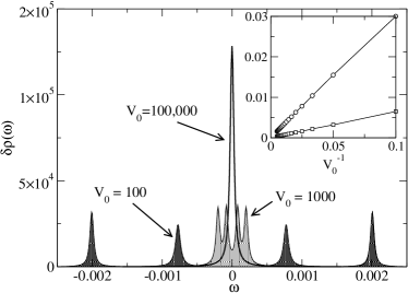
Figure 2: Change in the quasiparticle density of states arising from impurities separated by ${\bf R}=(2,2)$ as a function of energy $\omega/t$ for scattering potential $V_{0}=10^{6}t$. Inset: Scaling of the resonance peak energies as a function of $V_{0}$. The DOS for ${\bf R}=(2,0)$ is almost identical. Energies are measured in units of $t$, and $\Delta_{0}=0.1t$.

In this section, we derive expressions for the density of states for two impurities in a half-filled band. The discussion focusses on the unitary limit $V_{0}\rightarrow\pm\infty$. The half-filled tight-binding band possesses a particular global nesting symmetry yashenkin $\hat{\tau}_{2}\hat{G}^{0}({\bf k}+{\bf Q},\omega)\hat{\tau}_{2}=-\hat{G}^{0}({\bf k},\omega)$, with ${\bf Q}=(\pi,\pi)$ which is satisfied at $\omega=0$. For simplicity, we call this the $\tau_{2}$ symmetry. Potential scattering violates this symmetry, but in the case of infinite potential, impurity sites are effectively removed from the lattice, and the symmetry is recovered for any disorder configuration at $\omega=0$. In real space (see eg. otherdivergence )the $\tau_{2}$ symmetry may be expressed as

$$\hat{\tau}_{2}\hat{G}({\bf r},{\bf r}^{\prime},\omega)\hat{\tau}_{2}=-e^{i{\bf Q}\cdot({\bf r}-{\bf r}^{\prime})}\hat{G}({\bf r},{\bf r}^{\prime},\omega).$$ (8)

It will be useful to decompose the square tight-binding lattice into the usual two interleaved sublattices (denoted A and B). The phase factor on the right hand side of Eq. (8) is $+1$ if ${\bf r}$ and ${\bf r}^{\prime}$ belong to the same sublattice, and $-1$ otherwise.

The simplest quantity of interest is the quasiparticle density of states

$$\rho(\omega) = \sum_{n}[\delta(\omega-E_{n})+\delta(\omega+E_{n})]$$

$$= \rho_{0}(\omega)+\delta\rho(\omega),$$

where $E_{n}$ are the positive energy eigenvalues of the superconducting Hamiltonian, $\rho_{0}(\omega)$ is the DOS of the disorder-free system and $\delta\rho(\omega)$ is the change induced by the impurities. The DOS is related to the 2-impurity T-matrix defined in Eq. (3) by the phase shift $\eta(\omega)$hewson :

$$\delta\rho(\omega)=\frac{1}{\pi}\frac{\partial\eta}{\partial\omega},$$ (9)

where $\eta$ is given by,

$$\eta(\omega)=\tan^{-1}\frac{\mbox{Im }\det{\bf\hat{T}}}{\mbox{Re }\det{\bf\hat{T}}}$$ (10)

and the determinant is over spatial and spin indices.

We start with a discussion of two impurities belonging to one of the sublattices. The two impurities are at ${\bf R}_{1}$ and ${\bf R}_{2}$ with ${\bf R}\equiv{\bf R}_{1}-{\bf R}_{2}=(m,n)=$(even,even) or (odd,odd). The two-impurity T-matrix defined in Eq. (3) is particularly simple in this case:

$${\bf\hat{T}}=\frac{1}{D}\left[\begin{array}[]{cc}-G^{0}_{0}(0,\omega)\hat{\tau}_{0}&G^{0}_{0}({\bf R},\omega)\hat{\tau}_{0}\\ G^{0}_{0}({\bf R},\omega)\hat{\tau}_{0}&-G^{0}_{0}(0,\omega)\hat{\tau}_{0}\end{array}\right]$$

where $D=G^{0}_{0}(0,\omega)^{2}-G^{0}_{0}({\bf R},\omega)^{2}$. Noting that

$$\det{\bf\hat{T}}=\frac{1}{D^{2}},$$

we keep the leading order terms in $G_{0}({\bf R},\omega)$ as $\omega\rightarrow 0$, given explicitly in Eq. (5) and (6) and find that $\det{\bf\hat{T}}$ diverges as

$$\det{\bf\hat{T}}\rightarrow\left\{\begin{array}[]{ll}[2\omega C_{0}({\bf R})G^{0}_{0}(0,\omega)]^{-2}&{\bf R}=(\mathrm{even,even})\\ G^{0}_{0}(0,\omega)^{-4}&{\bf R}=(\mathrm{odd,odd})\end{array}\right.$$

and (analytically continuing $\omega$ to the real axis)

$$\delta\rho(\omega)\rightarrow\left\{\begin{array}[]{ll}1/[\omega\log^{2}(\Lambda/\omega)]&{\bf R}=(\mathrm{even,even})\\ 2/[\omega\log^{2}(\Lambda/\omega)]&{\bf R}=(\mathrm{odd,odd})\end{array}\right.$$ (11)

Because of the similarity of the approaches, we are able to compare our findings with those of PLpepinlee in some detail. Although the form of Eq. (11) is suggestive of the asymptotic result of PL for the disorder-averaged limit, its origin is quite different. This difference is easiest to see for the (odd,odd) impurity configuration: here the local Green’s function $\hat{G}^{0}(0,\omega)$ is dominant over the nonlocal term $\hat{G}^{0}({\bf R},\omega)$ and the physics of the low energy resonance is essentially that of two non-interacting impurities. The total weight of the resonance is therefore twice that of a single impurity. For the (even,even) case the situation is a little more complicated, since the local and nonlocal terms are nearly equal in magnitude; interference effects reduce the spectral weight of the combined resonance to half that of two isolated resonances. In both cases the situation is quite different from Ref. pepinlee where the logarithmic divergence arises from averaging over all possible impurity separations using the approximate form $\hat{G}^{0}({\bf R},\omega)\sim 1/R$ out to a cutoff $\sim t/R$. The PL result is inherently nonlocal.

Numerical calculations for two impurities with separation ${\bf R}=(2,2)$ are shown in Fig. 2. For $V_{0}=100t$, four clearly defined peaks are seen, corresponding to the level splitting of the single impurity resonances of the isolated impuritieszhutwoimpurity . As shown in the inset, the peak positions scale strongly with $V_{0}$, and a single peak appears only when $V_{0}\sim 10^{5}t$.

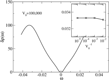
Figure 3: Change in the quasiparticle density of states for impurities separated by ${\bf R}=(2,1)$ as a function of energy $\omega/t$ for scattering potential $V_{0}=10^{6}t$ and $\Delta_{0}=0.1t$. Inset: Scaling of the resonance peak position as a function of $V_{0}$.

We continue now with the case where the impurities belong to different sublattices and are separated by ${\bf R}=$(even,odd). The two-impurity T-matrix defined in Eq. (3) is:

$${\bf\hat{T}}=\frac{1}{D^{\prime}}\left[\begin{array}[]{cc}-G^{0}_{0}(0,\omega)\hat{\tau}_{0}&C_{1}({\bf R})\hat{\tau}_{1}+C_{3}({\bf R})\hat{\tau}_{3}\\ C_{1}({\bf R})\hat{\tau}_{1}+C_{3}({\bf R})\hat{\tau}_{3}&-G^{0}_{0}(0,\omega)\hat{\tau}_{0}\end{array}\right]$$

with $D^{\prime}=G(0,\omega)^{2}-C_{1}({\bf R})^{2}-C_{3}({\bf R})^{2}$. It follows easily that $\det{\bf\hat{T}}={D^{\prime}}^{-2}$ and that

$$\delta\rho(\omega\rightarrow 0)\propto\frac{d}{d\omega}\left(\omega^{2}\ln\frac{\Lambda}{\omega}\right)\rightarrow 0$$ (12)

A similar result holds for ${\bf R}=$(odd,even). Physically, the fact that $\delta\rho$ vanishes at the Fermi level indicates that bound state energies must always arise at nonzero energies. Numerical calculations of the DOS shown in Fig. 3 demonstrate that there is no remnant of the single impurity $\omega\rightarrow 0$ divergence for this orientation, and that the resonance energies scale very little with $V_{0}$. In this case, it is the dominance of the nonlocal terms which shifts the resonance to finite energy.

III Disordered system with global particle-hole symmetry

In this section, we discuss the correspondence between the two impurity problem and the disordered $d$-wave superconductor. There are two separate issues to be dealt with. The first has to do with the nature of the divergence at $\omega=0$ which occurs in the tight-binding model, while the second has to do with the more general question of how the impurity band evolves with impurity concentration. For these calculations, we numerically diagonalize the mean-field Hamiltonian for a random distribution of impurities, under the assumption of a homogeneous order parameter for a finite sized $L\times L$ system with periodic boundaries. For a detailed description of the method, we refer the reader to eg. atkinsonops . We retain the eigenenergies $E_{n}$ and the eigenvectors

$$\Psi^{(n)}({\bf r})=\left(\begin{array}[]{c}u^{(n)}({\bf r})\\[5.69054pt] v^{(n)}({\bf r})\end{array}\right).$$

The total density of states is just $\rho(\omega)=\sum_{n}\delta(\omega-E_{n})$, and the single-spin LDOS is

$$\rho({\bf r},\omega)=\sum_{n}|u^{(n)}({\bf r})|^{2}\delta(\omega-E_{n}).$$

Since there is no moment formation, $\sigma=\uparrow$ and $\sigma=\downarrow$ are equivalent.

The Green’s function $G^{0}({\bf k},\omega=0)$ for the Hamiltonian (1a) (with $\mu=0$) has the special symmetry $\hat{\tau}_{2}\hat{G}^{0}({\bf k}+{\bf Q},0)\hat{\tau}_{2}=-G^{0}({\bf k},0)$ where ${\bf Q}=(\pi,\pi)$ is the antiferromagnetic wavevector. The $\tau_{2}$ symmetry is requiredatkinsondetails ; yashenkin for the divergence in $\rho(\omega\rightarrow 0)$. This symmetry is only strictly satisfied when $L$ is evenparity , and an even-odd oscillation at the Fermi level as a function of $L$ is clearly evident in our numerical work. Throughout this paper, we restrict ourselves to even $L$.

III.1 Divergence at $\omega=0$

Figure 4: Total density of states for $n_{i}=0.1$. (a) DOS for $V_{0}=100t$ (solid) and $L=60$. Eq. (13) is plotted for comparison (dashed line). (b) Scaling of DOS with $V_{0}$. $\rho_{PL}(\omega)$ is again plotted for comparison. (c) Scaling of DOS with $L$. (d) Scaling of DOS with $V_{0}$ for $V_{0}/t=100,\,500,\,1000,\,5000,\,10^{4},\,10^{5},\,10^{6}$ and $L=60$. A background $\rho_{0}=0.25t^{-1}$ has been subtracted. The figure shows that the density of states is a peaked function whose width scales as $1/V_{0}$ and whose height scales as $V_{0}$, suggesting that $\lim_{V_{0}\rightarrow\infty}\rho(\omega)\sim\delta(\omega)$. All energies are in units of $t$.

The DOS for a large concentration $n_{i}=0.1$ of strong scattering impurities in a $d$-wave superconductor is shown in Fig. 4. The figure is restricted to low energies, and shows only the zero-energy peak at the Fermi level, and a small portion of the impurity band. For comparsion, the $d$-wave gap has an energy $\Delta_{0}=0.2t$ and the gap edge in the tunneling density of states is $0.4t$. For clarity, we often make a distinction between states in the peak and states in the impurity band, by which we mean states belonging to the DOS plateau which is characterized by a constant density of states $\rho_{0}$. In Fig. 4(a), for example, $\rho_{0}\approx 0.25t^{-1}$.

In Fig. 4(a), the total DOS is shown for an impurity potential $V_{0}=100t$ corresponding to a strong scattering potential. The results are in quantitative agreement with earlier numerical workatkinsondetails ; Zhu . The PL result

$$\rho_{PL}(\omega)\approx\frac{n_{i}}{|\omega|[\ln^{2}(\Lambda/\omega)+(\pi/2)^{2}]},$$ (13)

is also shown. Here, we take $\Lambda=1$, first because this was the cutoff used in previous numerical workZhu and, second, because this gives a good fit to the numerics at $V_{0}=100t$. It should be clear from Figs. 4(a) and (b) however, that although the fit is striking at $V_{0}=100t$, it is less so for other values of $V_{0}$. In our numerics, we find a smooth evolution of the low energy peak as a function of $V_{0}$ and there is no value of $V_{0}$ beyond which the asymptotic behaviour saturates. In general, $\rho_{PL}(\omega)$ does not appear to fit the data well, except for certain special parameter sets.

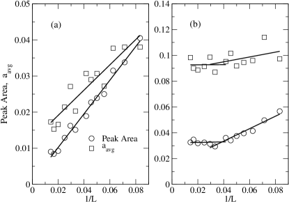
Figure 5: Scaling of the peak area and inverse participation ratio with system size $L$ and $V_{0}=10^{6}t$. $a_{avg}$ is averaged over states with energies $10^{-5}t<E_{n}<0.03t$. (a) Scaling for $n_{i}=0.1$. (b) Scaling for $n_{i}=0.2$. Solid lines are linear fits to the data. For these curves, $\Delta_{0}=0.5t$.

The shape of the peak at $\omega=0$ is modified by finite-size effects. There is a crossover in behaviour which occurs when the mean level spacing in the impurity band $\delta_{L}=1/(\rho_{0}L^{2})$ is comparable to the peak width. Scaling of the DOS is shown for $V_{0}=250t$ in Fig. 4(c). The peak height scales with $L$ for $L\lesssim 40$ and saturates at larger system sizes. The implication is that some care must be taken in approaching the $V_{0}\rightarrow\infty$ limit.

The unitary limit of the infinite system may be approached in two ways. First, one may consider taking $\lim_{V_{0}\rightarrow\infty}\lim_{L\rightarrow\infty}$ so that the level spacing in the impurity band is much less than the peak width. Second, one may consider taking the limit $L\rightarrow\infty$ with $V_{0}=\infty$. In the first approach, the $\tau_{2}$ symmetry is only strictly satisfied when $L=\infty$, while in the second approach, the $\tau_{2}$ symmetry is rigorously satisfied for any even value of $L$. For this reason, we view the second approach as preferable.

The limit $V_{0}\rightarrow\infty$ for fixed $L$ is illustrated in Fig. 4(d). The data are scaled by the impurity potential, and the general trend is that as $V_{0}$ is increased, a sharp peak develops at $\omega=0$. Furthermore, the peak scales as $\rho(\omega)\approx V_{0}F(\omega V_{0})$, implying that

$$\lim_{V_{0}\rightarrow\infty}\rho(\omega)\sim\delta(\omega).$$ (14)

Not surprisingly, the weight contained in the delta-peak in the $V_{0}\rightarrow\infty$ limit scales with $L$, as shown in Fig. 5. For $n_{i}=0.1$, this scaling is consistent with what we found in Fig. 4(c). When $n_{i}=0.2$, on the other hand, the peak area saturates when $L\gtrsim 40$, which is not expected since the peak width is still many orders of magnitude smaller than the typical level spacing $\delta_{L}$ in the impurity band. To learn more about the origin of this saturation we plot in the same figure the scaling of the inverse participation ratio, defined by

$$a(\omega)=\sum_{n}\frac{\sum_{i}[u^{(n)}({\bf r}_{i})^{4}+v^{(n)}({\bf r}_{i})^{4}]}{\big{(}\sum_{i}[u^{(n)}({\bf r}_{i})^{2}+v^{(n)}({\bf r}_{i})^{2}]\big{)}^{2}}\delta(\omega-E_{n}).$$

$a(\omega)$ scales as $L^{-d}$ for wavefunctions which are extended in $d$-dimensions, and does not scale with $L$ for localised states. The localization length is typically extracted from the crossover which occurs when $L\approx\xi_{L}$ where $\xi_{L}$ is the localization length. As we shall see below, states in the delta-peak behave differently from those in the impurity band, and we find that the peak area is correlated with the localization properties of the impurity band. In Fig. 5, the inverse participation ratio is averaged over states in a narrow energy window adjacent to (but not including) the delta peak. It is evident from the figure that for $n_{i}=0.2$, a crossover to the localized regime occurs, and we can extract a localization length $\xi_{L}\approx 40$.

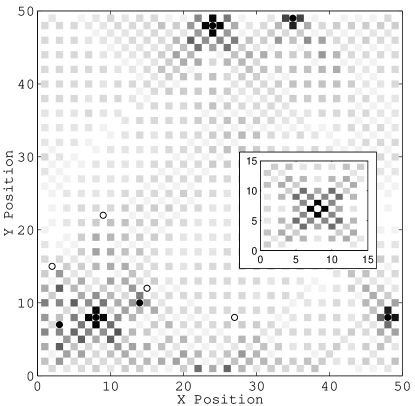
Figure 6: Local density of states for 0.4% concentration of impurities and $|E_{n}|<10^{-5}t$ (4 eigenvalues). Impurity locations on sublattice A are indicated with open circles, those on sublattice B with filled circles, and the impurity potential is $V_{0}=10^{6}t$. Inset: The inset shows a detail of the LDOS for a single impurity.

Remarkably, we find that the area of the $\delta$-peak appears to saturate when $L>\xi_{L}$. This situation is analogous to one reported earlier in $d$-wave superconductors possessing no special symmetries. There, it was shown that quantum interference (arising from “maximally crossed” diagrams) leads to a suppression of the DOS at the Fermi levelfisher over an energy scale $\delta_{\xi_{L}}=1/(\rho_{0}\xi_{L}^{2})$ (This situation is illustrated in Fig.1(b)). In finite size systems, the energy scale for the DOS suppression is actually $\delta_{L}$ and the scaling of the suppression saturates when $L>\xi_{L}$atkinsondetails .

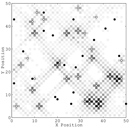
Figure 7: Local density of states for 2% concentration of impurities and $|E_{n}|<10^{-5}t$ (20 eigenvalues). Impurity locations on sublattice A are indicated with open circles, those on sublattice B with filled circles, and the impurity potential is $V_{0}=10^{6}t$.

We note that the origins of the delta-peak divergence are fundamentally different from those discussed in PL, where the divergence arises from the cumulative effects of interference between a large number of distant impurities. Here the result appears to be a mesoscopic effect which survives because localization makes the effective system size finite. However, although the delta-peak result is different from earlier predictions for a continuous divergence at the Fermi level, it does not preclude the existence of an additional divergent term which is unobservable because of finite system size effects. Indeed, if we consider the effect of finite system size on the PL result we find the interference between distant impurities is cut off by $L$ and we should make the substitution $\omega\rightarrow\max(\omega,t/L)$ in $\rho_{PL}$, implying a cutoff energy $\omega_{c}\approx t/L$ below which the DOS saturates. By this estimate, the contribution to the plot in Fig. 4 is cut off below $\omega_{c}\approx 0.017t$, suggesting that the PL peak should be unobservable.

It is particularly instructive to consider the structure of the delta-peak divergence in real space. Figure 6 shows the combined local density of states from the eigenstates with energy $|E_{n}|<10^{-5}t$ which make up the delta-peak (these states are well-separated from all other eigenvalues). For a single impurity (shown in the inset) the zero-energy resonance has a fourfold spatial structure with bright lobes on sites adjacent to the impurity along the antinodal (100) and (010) crystal directions, and extended tails in the nodal (110) and ($1\overline{1}0$) directions, in agreement with many earlier calculationsBalatsky . For 0.4% disorder (10 impurities), the situation is quite different; even at this relatively low concentration, there is significant interference between impurities. We see four pronounced zero-energy resonances, but the remaining six impurities are—at best—only weakly visible. For each of the visible resonances, the LDOS has the superficial structure of the isolated impurity LDOS, with maxima appearing in the antinodal direction and tails extending away from the impurities in the nodal directions. However, there is no obvious correlation between the degree of isolation and the appearance of a zero-energy resonance. Indeed, of the four strong resonances, only two are more than 10 lattice sites from the nearest impurity. For 2% disorder (50 impurities), shown in Fig. 7, the situation is similar. Only a small fraction of impurities contribute to the zero-energy LDOS and, again, the visible resonances do not necessarily belong to the most isolated impurities. At this higher impurity concentration, however, a definite pattern in the LDOS is observable. Long tails along the $(110)$ and $(1\overline{1}0)$ directions give the appearance of a network of impurities.

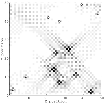
Figure 8: Local density of states for 0.5% impurities and $V_{0}=10^{6}t$ derived from a single eigenvalue with $E_{n}=0.0318t$.

Remarkably, we find that all impurities within the visible network in Fig. 7 belong to one sublattice, arbitrarily denoted A, while the remaining impurities belong to the B sublattice. Similarly, in Fig. 6, all visible impurities belong to the B sublattice. While this is reminiscent of the two-impurity problem discussed in the previous section, it is also quite surprising. For the two-impurity problem, it was shown that the zero-energy resonance is preserved when both impurities inhabit the same sublattice and is destroyed otherwise. The natural extrapolation is that, for a random distribution of many impurities, every impurity is expected to have have some reasonably close neighbor belonging to the other sublattice which contributes to the destruction of the zero-energy peak. Clearly, this does not happen. Instead, the impurities belonging to the A sublattice for this sample are dominant at $\omega=0$ for reasons we do not completely understand at present. An apparent consequence of this dominance is that the resonances of impurities belonging to the B sublattice are shifted to higher energies. We speculate, but cannot prove, that the system in the thermodynamic limit will have “domains” of typical size $\xi_{L}$ in which either A or B impurities are resonant.

The observed networks are also reminiscent of an earlier proposalBalatskySalkola that impurities form networks from single impurity resonances which lead to a delocalization transition as $\omega\rightarrow 0$. Numerical scaling calculationsZhu for a finite impurity potential ($V_{0}=100t$) did not find such a transition, however, nor does the present work (see below). In any case, we emphasize that the sharply defined networks exhibited above are a feature of Hamiltonians with $\tau_{2}$ symmetry only, and not a general feature of $d$-wave superconductors as suggested in BalatskySalkola .

III.2 Impurity band away from $\omega=0$

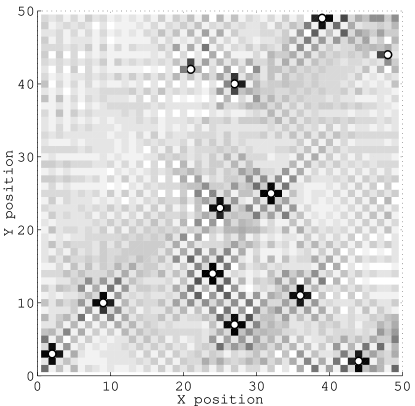
Figure 9: Local density of states for 0.5% impurities and $V_{0}=10^{6}t$ averaged over 5 eigenvalues in the energy interval $|E_{n}-0.03t|<0.02t$.

We now turn our attention to the states in the impurity band away from $\omega=0$. The previous analysis raises some interesting questions about the formation of this “band”. Is the $\omega>0$ DOS plateau formed, as Figures 6 and 7 perhaps suggest, by summing over many impurities, some of which are resonant at a given energy and others not? This would imply that, as energy was scanned in STM experiments, different impurities would “light up” – become resonant–and turn off at different energies within the impurity band, a scenario we will refer to as “inhomogeneous broadening” of the impurity resonances. Experimental data davisnative ; davisZn indicate instead that all impurities, regardless of local environment, appear to be resonant all through the impurity band, i.e. that each local spectral function is qualitatively similar in position and width, i.e. “homogeneous broadening”. In addition, there is some evidence from explicit Zn substitutiondavisZn that the number of impurity resonances corresponds closely to the number of Zn atoms introduced into the crystal, i.e. there are no atoms which do not light up. It is for this reason that interpretations have typically been given in terms of one-impurity models. However, in the same experiments the width of spectral features is roughly an order of magnitude larger than those predicted by the simplest one-impurity models.

These apparent paradoxes can be resolved by recognizing that the energy range probed by STM, although very small ($\cal{O}$(0.1meV)) in laboratory terms, is still large enough to sample an essentially infinite number of eigenstates of the macroscopic system. In Fig. 8 we show the LDOS derived from a single eigenstate at an energy which is in the impurity band, but away from the zero-energy delta-peak. Two features of this figure stand out. First, as was the case at $\omega=0$, only a fraction of the impurities contribute to any given eigenstate. Second, the extended tails which were are important in the formation of the delta-peak are blurred by the incommensurability between the lattice and the wavevectors contained in the eigenstate. As we move further away from $\omega=0$, this incommensurability becomes more pronounced and the tails become increasingly blurred.

The inequivalency between impurities in Fig. 8 is surprising not only because STM provides little evidence for such a picture, but also because the arguments about the formation of networks fail when $\omega\neq 0$ (indeed, there is no visible network in the figure). When one now averages the LDOS over a small energy window, as in Fig. 9, the system starts to look much more homogeneous, in the sense that all impurities contribute visible resonances with the classic fourfold symmetry. The window width is small compared to the impurity band, and we have checked that the pattern averaged in this way remains roughly the same up to energies of order the impurity band itself, $\gamma\simeq 0.25t$ for the parameter set of the figure. Thus, it appears as if there is an important distinction between individual eigenstates which determine, for example, localization properties, and averages over finite energy windows which determine the tunneling spectrum.

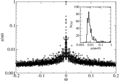
Figure 10: Inverse participation ratio $a(\omega)$ for $n_{i}=0.1$, $V_{0}=10^{6}$ on a $30\times 30$ lattice with 50 configurations. States in the impurity band for $|E_{n}|\gtrsim t/V_{0}$ have approximately uniform spatial extent. States with $|E_{n}|V_{0}\lesssim t$ exhibit strong fluctuations in spatial extent. Note that states with $a(E_{n})=1$ are confined to a single site, while states with $a(E_{n})\sim N^{-1}$ have a uniform spatial distribution. Inset: A histogram of the distribution of $a(\omega)$ for states in the zero-energy $\delta$-function. Note the logarithmic horizontal axis.

Finally, in order to solidify the connection between local and bulk properties of the disordered system, the energy dependence of the inverse participation ratio is plotted in Fig. 10. For each impurity configuration, $a(E_{n})$ is calculated for all the eigenstates in the spectrum, and the aggregate is shown for 50 impurity configurations in the figure. There is a clear distinction between states inside and outside of the $\delta$-peak. States outside the $\delta$-peak are clearly extended (the localization length is much larger than the system size) and the distribution of $a(\omega)$ is relatively narrow at a given energy. On the other hand, there is a broad distribution of $a(\omega)$ in the $\delta$-peak, indicating a mix of localized and extended states. The figure inset shows a histogram of the distribution that demonstrates that most of the spectral weight in the $\delta$-peak comes from the extended tails of the resonances (Fig. 7) and not from the highly-visible localized resonances.

IV Conclusions

In this work we have studied the unitary limit of a disordered, half-filled $d$-wave superconductor with tight binding band. This model has a particular symmetry which is known to lead to a divergence in the density of states at the Fermi level, although the particular form of the divergence is controversial. We began with a discussion of the two-impurity problem, which yields an analytical solution in the $\omega\rightarrow 0$ limit. We found that, owing to the commensurability of the nodal wavevectors and the tight-binding lattice, there is an even-odd oscillation in the two-impurity density of states in the unitary (infinite scattering potential) limit. Impurity pairs on the same sublattice have a zero-energy divergence in the DOS similar to the single-impurity divergence. The origin of this divergence is quite different from that reported earlierpepinlee , which arises from the cumulative interference of a large number of distant impurities.

We also noted that for impurities located on different sublattices, the zero-energy single-impurity resonance is shifted to higher energies as a result of interference. Based on this result alone, it is natural to assume that, in the many impurity limit, any remnant of the single impurity peak will be obliterated since each impurity is expected to have at least one reasonably near neighbor which lies on the other sublattice. Surprisingly, we found that this is not the case. Exact numerical studies of finite-size systems show that unitary impurities actually form two interleaved networks on the A and B sublattices, one of which contains spectral weight at $\omega=0$, while the other does not. Away from $\omega=0$, quasiparticle eigenstates are no longer commensurate with the lattice, networks connecting resonant states along the nodal directions are smeared, and individual eigenstates consist of distorted resonances, which are inhomogeneously distributed. When the LDOS is averaged over a small window in energy, however, as in an STM experiment, the fourfold nature of the 1-impurity resonances is qualitatively recovered, and resonances on individual impurity sites appear remarkably similar, provided the impurities are not in immediate proximity. Although the resonance peak positions may be qualitatively related to the resonant energies of the underlying 1-impurity model, the widths are very different, of order the impurity bandwidth, given in the unitarity limit by $\gamma\simeq n_{i}\sqrt{\Delta_{0}E_{F}}$.

The $\omega>0$ states of the tight-binding band are generic in the sense that they do not posses the $\tau_{2}$ symmetry, or any other symmetry which is not present in high $T_{c}$ superconductors. In this sense, our results should be qualitatively applicable to the experiments on real cuprate materials. They suggest that the ability of one-impurity models of any kind to explain the details of local STM spectra in samples with per cent level disorder are severely limited. To substantiate this picture, it will be useful to compare local spectra on sites (e.g. impurity or nearest neighbor sites) around different impurities using realistic bands. Numerical calculations to realize the large systems necessary to obtain the resolution required to reach definite answers to these questions are in progress.

Acknowledgements This work was partially supported by NSF grant NSF-DMR-9974396, the Alexander von Humboldt Foundation, and by Research Corporation grant CC5543. PH and LZ would also like to thank J. Mannhart and Lehrstuhl Experimentalphysik VI of the University of Augsburg for hospitality during preparation of the manuscript.

V Appendix

The purpose of this appendix is to derive expressions for the Green’s function $G({\bf R},\omega)$ with ${\bf R}=(m,n)$, which are valid in the $\omega\rightarrow 0$ limit. The starting point is Eq. (2), and the first step is to express

$$\cos(k_{x}m) = 2^{m-1}\cos^{m}k_{x}$$

$$+\frac{1}{2}\sum_{j=1}^{[\frac{m}{2}]}(-1)^{j}\frac{m(m-j-1)!}{j!(m-2j)!}(2\cos k_{x})^{m-2j}$$

where $[\ldots]$ refers to the integer part of the argument. We focus on the half-filled case $\mu=0$ and write Eq. (2) as the sum of terms of the form

$$g_{pq} = \sum_{\bf k}\cos^{p}(k_{x})\cos^{q}(k_{y})\frac{\omega\hat{\tau}_{0}+\epsilon_{k}\hat{\tau}_{3}+\Delta_{\bf k}\hat{\tau}_{1}}{\omega^{2}-E_{\bf k}^{2}}$$

where $p=m,m-2,\ldots$ and $q=n,n-2,\ldots$. We proceed by linearizing the dispersion near the node at $(\pi/2,\pi/2)$ and making the coordinate transformation $E^{2}=\epsilon_{\bf k}^{2}+\Delta_{\bf k}^{2}$, $\tan\theta=\Delta_{\bf k}/\epsilon_{\bf k}$.

$$g_{pq} = \frac{\alpha}{2^{p+q}}\int_{0}^{2\pi}\frac{d\theta}{2\pi}\left(-\frac{\sin\theta}{\Delta_{0}}-\frac{\cos\theta}{2t}\right)^{q}\left(\frac{\sin\theta}{\Delta_{0}}-\frac{\cos\theta}{2t}\right)^{p}$$

$$\times\int_{0}^{\Lambda}E^{p+q+1}dE\frac{\omega\hat{\tau}_{0}+E(\cos\theta\hat{\tau}_{3}+\sin\theta\hat{\tau}_{1})}{\omega^{2}-E^{2}},$$

The prefactor is $\alpha=N/(2\pi v_{F}v_{\Delta})$ where $N=4$ is the number of nodes, $v_{F}$ is the Fermi velocity and $v_{\Delta}$ is the anomalous quasiparticle velocity $|\nabla_{\bf k}\Delta_{\bf k}|$, and the cutoff $\Lambda$ is of order $\Delta_{0}$. The integrals over $E$ and $\theta$ are easily done and

$$g_{pq}(\omega)=\frac{-\alpha}{2^{p+q}}[\omega F_{p+q}(\omega)P^{0}_{pq}\hat{\tau}_{0}+F_{p+q+1}(\omega)(P^{3}_{pq}\hat{\tau}_{3}+P^{1}_{pq}\hat{\tau}_{1})]$$

where $P^{j}_{pq}$ are constants given by the angular integrations, and

$$F_{a}(\omega) = \int_{0}^{\Lambda}EdE\frac{E^{a}}{E^{2}-\omega^{2}}.$$

The constants $P^{j}_{pq}$ vanish for $j=1,3$ when $p+q=\mathrm{even}$ and vanish for $j=0$ when $p+q=\mathrm{odd}$. The first few nonzero elements are

$$P^{0}_{00} = 1$$

$$P^{1}_{10} = -P^{1}_{01}=\frac{1}{2\Delta_{0}}$$

$$P^{3}_{10} = P^{3}_{01}=-\frac{1}{4t}$$

$$P^{0}_{11} = P^{0}_{11}=-\frac{1}{2\Delta_{0}^{2}}+\frac{1}{8t^{2}}$$

Only even moments of $F_{a}(\omega)$ are needed:

$$F_{2n} = \sum_{j=0}^{n-1}\frac{\omega^{2j}\Lambda^{2(n-j)}}{2(n-j)}+\frac{\omega^{2n}}{2}\ln\frac{\Lambda^{2}}{-\omega^{2}}$$

Since we are interested in the leading order behavior of $G({\bf R},\omega)$ we note that for small $\omega$ ,

$$F_{0}(\omega) \rightarrow \frac{1}{2}\ln\frac{\Lambda^{2}}{-\omega^{2}}$$

$$F_{2n}(\omega) \rightarrow \frac{\Lambda^{2n}}{2n}$$

For ${\bf R}=(2m,2n)$, the leading order contribution to $G({\bf R},\omega)$ comes from the single term in the expansion containing $g_{00}$. To second order in $\omega$:

$$G({\bf R},\omega)=-(-1)^{n+m}\frac{\alpha\omega}{2}\ln\frac{\Lambda^{2}}{-\omega^{2}}\hat{\tau}_{0}+\omega C_{0}({\bf R})\hat{\tau}_{0},$$ (15)

where $C_{0}({\bf R})$ is real, and is the sum of several terms. The largest term contributing to $C({\bf R})$ is of order

$$\frac{\alpha|\omega|}{16(m+n)}\left(\frac{\Lambda}{\Delta_{0}}\right)^{2(m+n)}$$

from which we estimate a range of validity

$$|\omega|\lesssim\Lambda e^{-\frac{(\Lambda/\Delta_{0})^{2(m+n)}}{16(m+n)}}.$$

For other ${\bf R}$, there is no single dominant term in the expansion for the Green’s function, and the leading order behavior comes from the sum over a large number of real nondivergent terms. For our purposes, it is sufficient to note that when ${\bf R}=(2m+1,2n+1)$, the sums take the form

$$G({\bf R},\omega)=\omega C_{0}({\bf R})\hat{\tau}_{0},$$ (16)

and when ${\bf R}=(2m+1,2n)$ or $(2m,2n+1)$

$$G({\bf R},\omega)=C_{1}({\bf R})\hat{\tau}_{1}+C_{3}({\bf R})\hat{\tau}_{3},$$ (17)

where $C_{0}({\bf R})$, $C_{1}({\bf R})$, and $C_{3}({\bf R})$ are real constants.

References

- (1) Ali Yazdani, C. M. Howald, C. P. Lutz, A. Kapitulnik, and D. M. Eigler, Phys. Rev. Lett. 83, 176 (1999).
- (2) E.W. Hudson, S.H. Pan, A.K. Gupta, K-W Ng, and J.C. Davis, Science 285, 88 (1999)
- (3) S. H. Pan, E. W. Hudson, K. M. Lang, H. Eisaki, S. Uchida, J. C. Davis, Nature, 403, 746 (2000).
- (4) T. Cren et al., Phys. Rev. Lett. 84, 147 (2000).
- (5) S.-H. Pan et al., Nature 413, 282 (2001).
- (6) K.M. Lang, V. Madhavan, J. E. Hoffman, E. W. Hudson, H. Eisaki, S. Uchida and J.C. Davis, Nature 415, 412 (2002).
- (7) C. Howald, P. Fournier, and A. Kapitulnik, Phys. Rev. B 64, 1005041 (2001).
- (8) C. Howald, H. Eisaki, N. Kaneko, A. Kapitulnik, cond-mat/0201546
- (9) J. E. Hoffman et al., Science 295, 466 (2002).
- (10) J. M. Byers, M. E. Flatté, and D. J. Scalapino, Phys. Rev. Lett. 71, 3363 (1993).
- (11) A. V. Balatsky, M. I. Salkola, and A. Rosengren, Phys. Rev. B 51 15 547 (1995).
- (12) See M.E. Flatté and J.M. Byers, Solid State Physics 53, 137-228 (1999).
- (13) Anatoli Polkovnikov, Subir Sachdev and Matthias Vojta, Phys. Rev. Lett. 86, 296 (2001).
- (14) J.X. Zhu, C.S. Ting, and C.R. Hu, Phys. Rev. B62, 6027 (2000).
- (15) I. Martin, A. V. Balatsky, and J. Zaanen, Phys. Rev. Lett 88, 097003 (2002).
- (16) D. Morr and Stavropoulos, cond-mat/0207243
- (17) Lingyin Zhu, W. A. Atkinson, and P. J. Hirschfeld, cond-mat/0208008.
- (18) P.J. Hirschfeld and W.A. Atkinson, J. Low Temp. Phys. 126, 881 (2002).
- (19) N. E. Hussey, Adv. Phys. 51, 1685 (2002).
- (20) A. A. Nersesyan, A. M. Tsvelik, and F. Wenger, Phys. Rev. Lett. 72, 2628 (1994).
- (21) T. Senthil and M.P.A. Fisher, Phys. Rev. B60, 6893 (1999).
- (22) W.A. Atkinson, P.J. Hirschfeld and A.H. MacDonald, Phys. Rev. Lett. 85, 3922 (2000).
- (23) K. Ziegler, M.H. Hettler, and P.J. Hirschfeld, Phys. Rev. Lett. 77, 3013 (1996).
- (24) C. Pépin and P.A. Lee, Phys. Rev. Lett. 81, 2779 (1998); Phys. Rev. B 63, 054502 (2001).
- (25) Claudio Chamon and Christopher Mudry, Phys. Rev. B 63, 100503-1 (2001).
- (26) M. Fabrizio, L. Dell’Anna, and C. Castellani, Phys. Rev. Lett. 88, 076603 (2002); A. Altland, Phys. Rev. B 65, 104525 (2002).
- (27) W.A. Atkinson, P.J. Hirschfeld, A.H. MacDonald, and K. Ziegler, Phys. Rev. Lett. 85, 3926 (2000).
- (28) A.G. Yashenkin, W.A. Atkinson, I.V. Gornyi, P.J. Hirschfeld, and D.V. Khveshchenko, Phys. Rev. Lett. 86, 5982 (2001).
- (29) İnanç Adagideli, Daniel E. Sheehy, and Paul M. Goldbart Phys. Rev. B 66 140512 (2002).
- (30) Y. Onishi, Y. Ohashi, Y. Shingaki, and K. Miyake, J. Phys. Soc. Jpn. 65, 675 (1996).
- (31) U. Micheluchi, F. Venturini and A. P. Kampf, cond-mat/0107621.
- (32) Jian-Xin Zhu, D. N. Sheng, and C. S. Ting, Phys. Rev. Lett. 85 4944 (2000).
- (33) Y. H. Yang, Y. G. Wang, M. Liu, and D. Y. Xing, cond-mat/0211590 (2002).
- (34) R. Joynt, J. Low Temp. Phys. 109, 811 (1997).
- (35) A. V. Balatsky and M. I. Salkola, Phys. Rev. Lett. 76, 2386 (1996); See also the comment by D. N. Aristov and A. G. Yashenkin, Phys. Rev. Lett. 80, 1116 (1998) and the reply A. V. Balatsky and M. I. Salkola, Phys. Rev. Lett. 80 1117 (1998).
- (36) A. C. Hewson, “The Kondo Problem to Heavy Fermions”, Cambridge Univ. Press (1993)
- (37) Christopher Mudry, P. W. Brouwer, Akira Furusaki, Phys. Rev. B 59 13221 (1999); K. Ziegler, W. A. Atkinson, P. J. Hirschfeld, Phys. Rev. B 64 54512 (2001).