Nanoscale phase separation in manganites

Abstract

We study the possibility of nanoscale phase separation in manganites in the framework of the double exchange model. The homogeneous canted state of this model is proved to be unstable toward the formation of small ferromagnetic droplets inside an antiferromagnetic insulating matrix. For the ferromagnetic polaronic state we analyze the quantum effects related to the tails of electronic wave function and a possibility of electron hopping in the antiferromagnetic background. We find that these effects lead to the formation of the threshold for the polaronic state.

1 Introduction

Manganites, the $\mathrm{Mn}$-based magnetic oxide materials such as $\mathrm{LaMnO}_{3}$, have been known for more than 50 years. Jonker and van Santen [1], and in more details Wollan and Koehler [2] investigated a rich magnetic structure of $\mathrm{Ca}$-doped $\mathrm{La}_{1-x}\mathrm{Ca}_{x}\mathrm{MnO}_{3}$ and conductivity in these materials. Specifically, a strong correlation between magnetic and transport properties in manganites was observed. These materials exhibit a metal-like resistance in a ferromagnetic phase and an insulating behavior in an antiferromagnetic phase.

While the variety of magnetic structures in manganites was explained by Goodenough [3] based on the theory of semicovalent exchange, the correlation between transport and magnetic properties was for a first time qualitatively explained by Zener [4]. He suggested that the conduction electrons travel in $\mathrm{La}_{1-x}\mathrm{Ca}_{x}\mathrm{MnO}_{3}$ through the Mn⁴⁺ ions and each ion carries a fixed magnetic moment which is strongly ferromagnetically coupled with the spin of a carrier by a generalized Hund rule. Since a spin of a conduction electron should be aligned parallel to the local spin, in the classical picture a conduction electron cannot move in antiferromagnetically ordered environment. Anderson and Hasegawa [5] solved a problem of two local spins and one conduction electron, providing a strong mathematical background to Zener ideas. They found that if the bare hopping amplitude was $t$, than a hopping amplitude of an electron moving between the two local spins is $t_{eff}=t\cos{\theta}$, where $\theta$ is an angle between the directions of the local spins. Thus, the kinetic energy of conduction electrons directly depends on an angle between the sublattice moments. Moreover, the conduction electrons tend to align ferromagnetically the local spins, which surround them. Hence, a competition between ferromagnetic coupling via a conduction electron (so called double exchange mechanism) and an antiferromagnetic coupling via superexchange of two neighboring local spins takes place. De Gennes [6] suggested that this competition results in a homogeneous canted state, namely an angle $\theta$ is uniform and monotonically changes from $\pi$ (collinear antiferromagnetic order) to $0$ (collinear ferromagnetic order) with increasing carriers concentration $x$. Based on these considerations de Gennes plotted the first phase diagram of the manganites.

Soon after this work, Nagaev [7, 8] improved de Gennes results by considering quantum fluctuations associated with the local spins. Nagaev proved that electron can move even in antiferromagnetically ordered phase with a small hopping amplitude $t/\sqrt{2S+1}$. Nagaev, Kasuya, and Mott also proposed [8, 9, 10, 11] that for small electron concentrations it is more favorable for conduction electrons to form a self-trapped state (ferromagnetic polaron or ferron) in antiferromagnetic matrix by creating a small ferromagnetic bubble, rather than to form a homogeneous canted state in the whole sample. Thus, it was one of the first hints for nanoscale phase separation in a double-exchange model made by that time.

Recent growth of interest in manganites was initiated in 1993 by the discovery of the colossal magnetoresistance (CMR) effect in doped LaMnO₃. The CMR phenomena implies a drastic decrease of resistivity in manganites in the presence of a magnetic field [12, 13]. Soon after discovery of CMR in manganites a phase diagram of $\mathrm{La}_{1-x}\mathrm{Ca}_{x}\mathrm{MnO}_{3}$ was revised [14]. It was found that a variety of phases appears in manganites in addition to those predicted by de Gennes.

There are plenty of experimental and theoretical studies of manganites nowadays. They were initiated first of all by the potential technological applications of colossal magnetoresistance phenomena and also by the interesting physics of strong correlations, which manifests itself in these materials. In particular, the interaction of spin, charge, and orbital degrees of freedom in manganites as well as their rich phase diagrams draw much attention of theorists and experimentalists in recent years.

The important question that has to be answered is about a leading mechanism responsible for CMR in the optimum doping region ($x\simeq 0.3$). Some authors argue that CMR could be explained in framework of the double-exchange mechanism alone [15], others [16] claim that it is necessary to take into account a lattice interaction (Jahn-Teller polarons), some insist that percolation-type arguments could explain CMR [17]. However, as it was pointed out by Dagotto et al[18] and Arovas and Guinea [19] both analytical and numerical calculations in various models related to manganites exhibit a strong tendency toward phase separation in the wide range of temperatures and concentrations. Thus, it is believed that CMR phenomena could be understood as a competition and co-existence of different phases in manganites as well as a phenomena related to the proximity of the optimum doping region to various phase-separation thresholds. Note that at higher concentrations close to half-filling there appears another threshold of phase separation in the system corresponding again to the formation of ferromagnetic droplets, but now in a charged ordered insulating matrix [20].

One of the authors [21] demonstrated that the double-exchange model at low doping is unstable toward phase separation and the energy of a homogeneous canted state is higher than an energy of a self-trapped state corresponding to a ferromagnetic polaron. Hence a legitimate question arises whether the stability of a polaronic state is preserved when quantum fluctuations of spins and tails of wave function of conduction electrons are taken into account.

2 Basic theoretical model

The general chemical formula of the most popular class of manganites is $\mathrm{Ln}_{1-x}\mathrm{A}_{x}\mathrm{MnO}_{3}$, where Ln is a trivalent cation Ln³⁺ (La, Pr, Nb, Sm, $\ldots$), and A²⁺ is a divalent cation (Ca, Sr, Ba, Mg, $\ldots$). Oxygen is in a O^2- state, and the relative fraction of Mn⁴⁺ and Mn³⁺ is controlled by a chemical doping $x$. This class of manganites has the perovskite structure. In the cubic lattice environment, the five-fold degenerate $3d$-orbitals of Mn-ions are split into three lower-energy levels ($d_{xy}$, $d_{yz}$, and $d_{zx}$), usually referred to as $t_{2g}$, and two higher-energy $e_{g}$ states ($d_{x^{2}-y^{2}}$ and $d_{3z^{2}-r^{2}}$). The $t_{2g}$ levels with three electrons form a state with a local spin $S=3/2$, whereas delocalized $e_{g}$ states contain an electron or are unoccupied depending on the chemical doping $x$. The $e_{g}$ states are further split by the static Jahn - Teller effect and for the simplicity we will treat here only the lowest $e_{g}$ state, assuming a Jahn-Teller gap to be large enough and neglecting any orbital effects in our consideration.

The simplest theoretical model suggested for the explanation of the properties of manganites is the ferromagnetic Kondo lattice model ($s-d$ model):

$$\hat{H}=-J_{H}\sum\limits_{i}\mathbf{S}_{i}\boldsymbol{\sigma}_{i}-t\sum\limits_{\langle i,\,j\rangle}Pc^{+}_{i\sigma}c_{j\sigma}P+J_{ff}\sum\limits_{\langle i,\,j\rangle}\mathbf{S}_{i}\mathbf{S}_{j}$$ (1)

The first term in equation (1) represents a strong on-site Hund’s ferromagnetic coupling ($J_{H}>0$) between the local spin $S=3/2$ and the spin of a conduction electron. In real manganites, the Hund’s interaction $J_{H}$ is of the order of 1 eV. The second term in equation (1) is the kinetic energy of the conduction electrons. The projection operator $P$ corresponds to the case of singly occupied $e_{g}$ orbitals (a strong Hund’s interaction prevents two conduction electrons with different spin projections from occupying the same site). Note that a strong electron-lattice interaction significantly reduces the effective width $W$ of the conduction band ($W=2zt$) resulting in a rather small hopping amplitude $t\approx 0.3$ eV. The third term in equation (1) is a weak antiferromagnetic coupling between local spins on neighboring sites, with $J_{ff}\sim 0.001$ eV. In equation (1), symbols $\langle i,j\rangle$ mean the summation over $z$ nearest neighbor sites.

In the case of a strong on-site Hund’s coupling ($J_{H}\gg W\gg J_{ff}$) the model described by the first two terms of the Hamiltonian (1) is referred to as the double exchange model. Note that if all local spins are ferromagnetically aligned, the conduction electrons will move freely in their surrounding. Thus, model (1) describes the competition between the direct antiferromagnetic coupling of local spins and the double exchange via conduction electrons, which tends to order local spins ferromagnetically. In the strong-coupling limit, Hamiltonian (1) can be simplified:

$$\hat{H}=-\sum\limits_{\langle i,\,j\rangle}t(\theta_{ij})a^{+}_{i}a_{j}+J_{ff}S^{2}\sum\limits_{\langle i,\,j\rangle}\cos(\theta_{ij})$$ (2)

where $a^{+}_{i}$ and $a_{j}$ are creation and annihilation operators of spinless fermions (conduction electrons whose spins $\sigma$ are aligned parallel to the local spins), $t(\theta_{ij})$ is an effective hopping amplitude, and $\theta_{ij}$ is an angle between sublattice moments, as we already discussed. The hopping amplitude in the case of classical spins ($S\gg 1$) reads:

$$t(\theta)=t\cos(\theta/2)$$ (3)

In Nagaev’s quantum approach the local spins at empty sites have the maximum projection, $+S$, on the magnetization vector of the corresponding sublattice. At occupied sites, however, local spin $\mathbf{S}$ and spin $\boldsymbol{\sigma}$ of a conduction electron form a state with the total spin $S+1/2$, but with two possible projections of it $S\pm 1/2$. So there are two effective bands in quantum canting corresponding to the two different projections of the total spin. Their bandwidths read [8, 21]:

$$t_{\pm}(\theta)=\frac{t}{2S+1}\left[\sqrt{2S+1+S^{2}\cos^{2}(\theta/2)}\pm S\cos(\theta/2)\right]$$ (4)

The quantum hopping amplitude drastically differs from the classical de Gennes one. In contrast to the de Gennes picture, an electron can still move through antiferromagnetic matrix creating a state with $S^{z}_{tot}=S+1/2$ at one site and a state with $S^{z}_{tot}=S-1/2$ at a neighboring site (a string-like motion introduced by Zaanen and Oleś [22]):

$$\left|S^{z}_{tot}=S+\frac{1}{2}\right\rangle\rightarrow\left|S^{z}_{tot}=S-\frac{1}{2}\right\rangle\rightarrow\left|S^{z}_{tot}=S+\frac{1}{2}\right\rangle\ldots$$

Hence, there are two equal hopping amplitudes in the case of electron motion through antiferromagnetic background: $t_{+}=t_{-}=t/\sqrt{2S+1}$. On the other hand, for ferromagnetic ordering one gets from equation (4) $t_{+}=t$ and $t_{-}=t/(2S+1)$. The proportionality of an effective bandwidth in the case of quantum canting to $1/\sqrt{S}$ is just an implication of its quantum nature.

3 Homogeneous canted state

An energy of the classical de Gennes state with an account taken for the antiferromagnetic interaction between the local spins reads:

$$E=-ztx\cos(\theta/2)+\frac{1}{2}zJ_{ff}S^{2}\cos(\theta),$$ (5)

where $z$ is the number of nearest neighbors, and $x$ is a carriers concentration. The first term in this equation is the gain in the kinetic energy, and the second term is the loss in the energy of antiferromagnetic interaction between local spins. Minimization of the energy (5) with respect to the parameter $\cos(\theta/2)$ yields:

$$E=-\frac{zt^{2}x^{2}}{4J_{ff}S^{2}}-zJ_{ff}S^{2},\qquad\cos(\theta/2)=\frac{tx}{2J_{ff}S^{2}}$$ (6)

Thus, we have a transition from a collinear antiferromagnetic state for $x=0$ to a collinear ferromagnetic state for $x=x_{c4}=2J_{ff}S^{2}/t$. For $0<x<x_{c4}$, the canting angle ($\theta\neq\pi$), and a homogeneous canted state takes place.

Previously, various homogeneous states were considered taking into account the quantum hopping amplitudes [8, 21]. In contrast to the classical case, a collinear antiferromagnetic state remains energetically favorable up to the critical value of the carrier concentration $x_{c1}$, which is given by:

$$x_{c1}=\frac{\pi^{4}}{3}\left[\frac{8J_{ff}S^{2}}{zt}\frac{1}{\sqrt{2S+1}}\right]^{3}$$ (7)

Thus, in a quantum case, the canted state occurs for $x>x_{c1}$, whereas in the classical case the canted state appears for arbitrarily low doping levels. At higher doping levels ($x>x_{c1}$), the two-band quantum canted state arises, namely conduction electrons are in the two bands with total spin projections $|S^{z}_{tot}=S+1/2\rangle$ and $|S^{z}_{tot}=S-1/2\rangle$. However at $x>x_{c2}\approx(27/2)x_{c1}$ the bottom of the second band lies above the chemical potential level and a one-band state of quantum canting becomes favorable [21]. Finally, at much higher carriers concentration ($x>x_{c3}=4J_{ff}S^{2}/t\sqrt{2S+1}$), a transition to the classical canted state of de Gennes (5) occurs. Note that for $x>x_{c4}=2J_{ff}S^{2}/t$ the canted state transforms into a collinear ferromagnetic state with the angle $\theta=0$.

To test the stability of the homogeneous state the electronic compressibility was calculated [21] according to the standard formula $\kappa^{-1}=d^{2}E/dx^{2}$. At very low concentrations $x<x_{c1}$ the compressibility is positive and a homogeneous collinear antiferromagnetic state corresponds to at least a local minimum of energy. However in the range of concentrations $x_{c1}<x<x_{c4}$ the compressibly $\kappa<0$ and the canted state is unstable. For example, we can calculate the compressibility of the classical de Gennes canted state and get:

$$\kappa^{-1}=-\frac{zt^{2}}{2J_{ff}S^{2}}<0.$$

Hence compressibility of this state is negative, i.e. de Gennes classical canted state is also unstable. The negative sign of the compressibility indicates the instability of homogeneous state toward the phase separation. The simplest case of nanoscale phase separation corresponds to the formation of small ferromagnetic polarons inside an antiferromagnetic matrix. This state was considered in Ref. [21, 23] and it was shown that a polaronic state is more favorable energetically than all the homogeneous states in the total range of concentrations $0<x<x_{c4}$. Note that magnetic polarons, in this case, correspond to the electron in the self-trapped ferromagnetic state of a finite radius inside an antiferromagnetic insulating matrix.

4 Polaronic state

As we already discussed, in the case of the classical hopping amplitude (3) a conduction electron may be self-trapped and form ferromagnetic droplets (magnetic polarons) inside an antiferromagnetic matrix. The simplest assumption is to consider that the boundary between the ferromagnetic region and the antiferromagnetic matrix is abrupt without an extended region of inhomogeneous canting. Then an energy of a polaronic state reads:

$$E=-tx\left(z-\frac{\pi^{2}a^{2}}{R^{2}}\right)+\frac{1}{2}zJ_{ff}S^{2}\,\frac{4\pi}{3}x\left(\frac{R}{a}\right)^{3}-\frac{1}{2}zJ_{ff}S^{2}\left[1-\frac{4\pi}{3}x\left(\frac{R}{a}\right)^{3}\right].$$ (8)

In equation (8), $R$ is a radius of a polaron and $a$ is a lattice constant. The first term in equation (8) describes the kinetic energy gain due to the formation of a ferromagnetic region. The corrections to this term proportional to $ta^{2}/R^{2}$ correspond to the localization energy of a conduction electron inside a ferromagnetic droplet of radius $R$. The second term in equation (8) is a loss in the Heisenberg antiferromagnetic energy of local spins inside the droplet. Finally, the third term describes the energy of an antiferromagnetic interaction between local spins in a region outside the ferromagnetic polarons. The polaron radius is obtained from the condition of energy minimization $dE/dR=0$. So we have the following expressions for an energy and a polaron radius:

$$E_{pol}=-ztx+\frac{5}{3}\pi^{2}tx\left(\frac{2zJ_{ff}S^{2}}{\pi t}\right)^{2/5}-\frac{1}{2}zJ_{ff}S^{2},$$ (9)

$$R_{pol}=a\left(\frac{\pi t}{2zJ_{ff}S^{2}}\right)^{1/5}$$ (10)

Note that in this case the transition from a polaronic to a ferromagnetic state occurs when ferromagnetic polarons start to overlap. The critical concentration for ferromagnetic transition reads:

$$x_{c5}=\frac{3}{4\pi}\left(\frac{a}{R}\right)^{3}=\frac{3}{4\pi}\left(\frac{2zJ_{ff}S^{2}}{\pi t}\right)^{3/5}$$ (11)

Figure 1: The electron wave function $\psi(r)$ and the canting angle $\theta(r)$ in the quantum case (solid lines) and the classical case (dashed lines).

Now, let us consider the quantum corrections to these results. In the case corresponding to the quantum hopping amplitude (4), a conduction electron can move through antiferromagnetic background with a heavy mass $m^{*}\sim\sqrt{S}$, so it is interesting to study for this case a problem concerning the stability of a magnetic polaron. Since the analysis of the discrete model (2) is rather complicated, we consider the continuum limit assuming that a radius of a polaron is much larger than the lattice constant $a$ (further on, we put $a=1$). A total energy (2) can now be written in the following form [24]:

$$E=-\int\left[z|\psi|^{2}+\psi^{*}\triangle\psi\right]t(\theta)dV+zJ_{ff}S^{2}\int\cos^{2}(\theta)dV,$$ (12)

$$t(\theta)=\frac{t}{2S+1}\left[\sqrt{2S+1+S^{2}\cos^{2}(\theta/2)}+S\cos(\theta/2)\right]$$ (13)

As one can see from equation (12), the total energy will lie between the two limiting values corresponding respectively to the motion of the conduction electron via ferromagnetic or antiferromagnetic backgrounds:

$$E_{FM}=-zt<E<E_{AFM}=-\frac{zt}{\sqrt{2S+1}}$$

Since the electron wave function should be normalized $\int|\psi|^{2}dV=1$, we minimize the functional $F=E-t\beta\int|\psi|^{2}dV$ with respect to parameters $\theta$ and $\psi$, where $\beta$ is a Lagrange multiplier. The corresponding Euler-Lagrange equations have the following form:

$$\left[2z\psi+\triangle\psi\right]t(\theta)+\triangle\left[t(\theta)\psi\right]-2\beta t\psi=0$$ (14)

$$\left[(z|\psi|^{2}+\psi^{*}\triangle\psi)\frac{\partial t(\theta)}{\partial\cos(\theta/2)}-2zJ_{ff}S^{2}\cos(\theta/2)\right]\sin(\theta/2)=0$$ (15)

We solve these two coupled differential equations by the following iterative procedure [24]: (a) we choose a trial function for the canting angle $\theta(r)$; (b) we solve the first differential equation (14) to obtain an electron wave function $\psi(r)$; (c) using an obtained value for $\psi(r)$ we solve equation (15) to get a canting angle function $\theta(r)$; (d) we return to the step (a) until our iteration process converges.

Functions $\psi(r)$ and $\theta(r)$ obtained by the numerical solution of equations (14) and (15) are shown in figure 1 for a broad range of the values of parameter $\alpha=t/J_{ff}S^{2}$. Note that exact numerical solution which takes into account both the effects of quantum canting and tales of the wave function coincides with the classical Nagaev-Mott solution for $\alpha\rightarrow\infty$. One can see that the magnetic polaron represents a very good localized object, and the transition region from the ferromagnetic ordering ($\theta=0$) to an antiferromagnetic matrix ($\theta=\pi$) is narrow enough. Nevertheless, a polaronic state can disappear at relatively small value of the parameter $\alpha_{c}\sim 75$. Indeed, as one can see from figure 2, there is a transition from the polaronic state to a collinear antiferromagnetic state at small values of parameter $\alpha<\alpha_{c}$. For this case, the total energy of a magnetic polaronic state is equal to the bottom of the band for electron motion through the antiferromagnetic background, and as a result for $\alpha<\alpha_{c}$ an electron can move freely through the antiferromagnetic matrix. Note that to get a more precise value of $\alpha_{c}$ we should solve a variational problem for the functional $F$ on the discrete lattice since for small values of $\alpha$ a continuous approximation is not accurate enough. The work along these lines is in progress now.

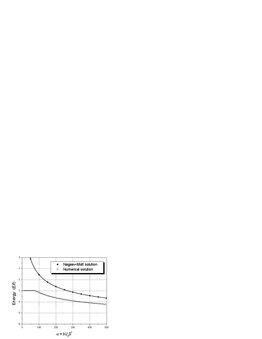
Figure 2: The ground state energy corresponding to polaron formation in the quantum case (open circles) and the classical case (solid circles). For local spin $S=3/2$ ferromagnetic and antiferromagnetic states correspond, respectively, to $E_{FM}=-6t$ and $E_{AFM}=-3t$.

5 Conclusion

The tendency toward phase-separation is very strong in the double-exchange model. We have shown that in the wide range of parameter $\alpha=t/J_{ff}S^{2}$ a conduction electron forms a self-trapped state. In this state, an electron is localized in the ferromagnetic droplet of finite radius embedded in the antiferromagnetic matrix. This construction seems rather natural in the de Gennes classical approximation of the double exchange, where hopping amplitude $t_{eff}=t\cos(\theta/2)$ and electron cannot move through an antiferromagnetic background since $t_{eff}=0$ for $\theta=\pi$. However, we have proved that even in the quantum case, when a conduction electron can travel slowly through antiferromagnetic matrix (since $t_{eff}=t/\sqrt{2S+1}$ for $\theta=\pi$), the polaronic state remains well defined and stable. Our approach to the one electron problem in an antiferromagnetic matrix corresponds to a very small doping region in real materials, where the concentration of charge carriers (e.g. holes in La_xCa_1-xMnO₃) is low. However we believe that even for higher concentrations the polaronic picture remains qualitatively correct. Moreover, at very low concentrations magnetic polarons should be localized on impurity sites [25] whereas at concentrations higher than the Mott threshold they are depinned from the impurities. Preliminary estimates show that the Mott threshold in manganites corresponds to $x_{M}\sim 0.01-0.04$, which is significantly lower than the critical concentration $x_{c5}\approx 0.15$ for the overlap of magnetic polarons.

Our model of polarons embedded in ferromagnetic matrix allows one also to calculate a magnetoresistance and a noise spectrum of manganites, if we suggest that an electron transport takes place via the hopping of electrons from one polaron to another, while a polaron itself is immobile. These calculations were carried out in Ref. [26, 27] and found experimental support in the recent paper of Babushkina et al[28].

If we proceed now to the experimental confirmation of small-scale phase separated picture we should mention that there already exist many evidences in favor of nanoscale phase separation in low and moderatly doped manganites. The confirmation of an inhomogeneous state in manganites comes from the nuclear magnetic resonance experiments of Allodi et al[29, 30], where the two different hyperfine lines corresponding to ferromagnetic and antiferromagnetic regions were observed. Experiments on neutron scattering of Biotteau et al[31] support the idea of small ferromagnetic droplets embedded in an antiferromagnetic or a canted matrix. And if we turn to transport properties, a very natural picture of electron percolation, which is in agreement with our model, was experimentally confirmed by Babushkina group in Ref. [32].

Thus the experimental and theoretical picture strongly confirms a phase-separated state in manganites in the region of low doping. Moreover, we believe that this picture remains qualitatively correct for the concentrations optimal for the CMR effect in the high temperature region $T>T_{C}$ ($T_{C}$ is a Curie temperature), where the ferromagnetic fluctuations of the short range (the temperature polarons) are present [23, 33]. Hence, a combination of very intuitive picture of polarons and the ideas of the percolation theory could provide a correct description for the behavior of manganites in the wide range of temperatures and carrier concentrations.

References

References

- [1] Jonker G H and Van Santen J H 1950 Physica (Utrecht) 16 337
- [2] Wollan E O and Koehler W C 1955 Phys. Rev.100 545
- [3] Goodenough J 1955 Phys. Rev.100 564
- [4] Zener C 1951 Phys. Rev.81 440; Zener C 1951 Phys. Rev.82 403
- [5] Anderson P W and Hasegawa H 1955 Phys. Rev.100 675
- [6] De Gennes P G 1960 Phys. Rev.118 141
- [7] Nagaev E L 1996 Phys. Usp. 39 781
- [8] Nagaev E L 1983 Physics of Magnetic Semiconductors (Moscow: Mir Publ.)
- [9] Nagaev E L 1967 JETP Lett. 6 18
- [10] Kasuya T 1970 Solid State Commun. 8 1635
- [11] Mott N F and Davis E A 1971 Electronic Processes in Non-Crystalline Materials (Oxford: Clarendon Press)
- [12] von Helmolt R, Wecker J, Holzapfel B, Schultz L and Samwer K 1993 Phys. Rev. Lett.71 2331
- [13] Jin S, Tiefel T H, McCormack M, Fastnacht R A, Ramesh R and Chen L H 1994 Science 264 413
- [14] Schiffer P, Ramirez A P, Bao W and Cheong S-W 1995 Phys. Rev. Lett.75 3336
- [15] Furukawa N 1997 J. Phys. Soc. Jpn. 66 2523
- [16] Millis A, Littlewood P B and Shraiman B I 1995 Phys. Rev. Lett.74 5144
- [17] Gor’kov L P and Kresin V Z 1998 JETP Lett. 67 985
- [18] Dagotto E, Hotta T and Moreo A 2001 Physics Reports 344 1
- [19] Arovas D and Guinea F 1998 Phys. Rev.B 58 9150
- [20] Kagan M Yu, Kugel K I and Khomskii D I 2001 JETP 93 415
- [21] Kagan M Yu, Khomskii D I and Mostovoy M V 1999 Eur. J. Phys.B 12 217
- [22] Zaanen J, Oleś A M and Horsch P 1992 Phys. Rev.B 46 5798
- [23] Kagan M Yu and Kugel K I 2001 Phys. Usp. 44 553
- [24] Pathak S and Satpathy S 2001 Phys. Rev.B 63 214413
- [25] Nagaev E L 1999 Physics Letters A 257 88
- [26] Rakhmanov A L, Kugel K I, Blanter Ya M and Kagan M Yu 2001 Phys. Rev.B 63 174424
- [27] Sboychakov A O, Rakhmanov A L, Kugel K I, Kagan M Yu and Brodsky I V 2002 JETP 95 753
- [28] Babushkina N A, Chistotina E A , Kugel K I, Rakhmanov A L, Gorbenko O Yu and Kaul A R 2003 J. Phys.: Condens. Matter15 259
- [29] Allodi G, De Renzi R, Guidi R, Licci R and Pieper M W 1997 Phys. Rev.B 56 6036
- [30] Allodi G, De Renzi R, Solzi M, Kamenev K, Balakrishnan G and Pieper M W 2000 Phys. Rev.B 61 5924
- [31] Biotteau G, Hennion M, Moussa F, Rodríguez-Carvajal J, Pinsard L, Revcolevschi A, Mukovskii Y M and Shulyatev D 2001 Phys. Rev.B 64 104421
- [32] Babushkina N A, Belova L M, Khomskii D I, Kugel K I, Gorbenko O Yu and Kaul A R 1999 Phys. Rev.B 59 6994
- [33] Krivoglaz M A 1972 Phys. Usp. 15 153