Nosé-Hoover sampling of quantum entangled distribution functions

Abstract

While thermostated time evolutions stand on firm grounds and are widely used in classical molecular dynamics (MD) simulations [1], similar methods for quantum MD schemes are still lacking. In the special case of a quantum particle in a harmonic potential, it has been shown that the framework of coherent states permits to set up equations of motion for an isothermal quantum dynamics [2]. In the present article, these results are generalized to indistinguishable quantum particles. We investigate the consequences of the (anti-)symmetry of the many-particle wavefunction which leads to quantum entangled distribution functions. The resulting isothermal equations of motion for bosons and fermions contain new terms which cause Bose-attraction and Pauli-blocking. Questions of ergodicity are discussed for different coupling schemes.

PACS: 05.30.-d; 05.30.Ch; 02.70.Ns

Keywords: Quantum statistics; Canonical ensemble; Ergodic behaviour; Thermostat; mixed quantum-classical system

1 Introduction and summary

Classical MD simulations are performed by solving Hamilton’s equations of motion numerically. Therefore, the internal energy of the system is conserved during time evolution. If the ergodic hypothesis is satisfied, a time average of a macroscopic observable is, under equilibrium conditions, the same as a microcanonical ensemble average. Hence, isoenergetic molecular dynamics entails a method for the calculation of microcanonical ensemble averages.

In the canonical ensemble, however, the internal energy of the system is not constant, but free to fluctuate by thermal contact to an external heat bath. In order to adapt classical MD simulations to the problem of the calculation of canonical ensemble averages, i. e. to pass over from an isoenergetic to an isothermal time evolution, powerful methods have been developed since the 1980s, and they are commonly used nowadays [3, 4]. Some of them, like the Nosé-Hoover chain technique [5] or the Kusnezov-Bulgac-Bauer thermostat [6], are based on deterministic time-reversal equations of motion leading to trajectories that fill the phase space of the system according to the canonical thermal weight. This allows the calculation of canonical ensemble averages by means of molecular dynamics.

In quantum mechanics, the problem is more involved, and the pioneering approaches of Grilli and Tosatti [7] and Kusnezov [8] were not applied very much. Moreover, the quantum mechanical time evolution itself is a hard computational problem. However, a number of approximate quantum MD methods are available [9]. It is an open question whether they can be modified in a manner appropriate to permit the calculation of quantum canonical averages.

In a different methodological approach to isothermal quantum dynamics, we have shown that in the special case of a quantum particle in a harmonic oscillator potential, the framework of coherent states permits to set up equations of motion for an isothermal quantum dynamics [2]. Following the approaches of Nosé and Hoover or the similar KBB-technique, time-dependent pseudofriction terms are added to the equations of motion for the parameters of coherent states. The dynamics of the pseudofriction coefficients is designed such that the desired thermal weight function is a stationary solution of a generalized Liouville equation on a mixed quantum-classical phase space.

The principle of indistiguishability of identical particles adds an important quantum aspect to the problem of isothermal quantum dynamics. The present article focusses on the modifications of the method presented in [2] for a system of two non-interacting identical particles. The (anti-)symmetry of the wavefunction leads to an entangled distribution function on quantum phase space. Surprisingly, we find that the originally classical Nosé-Hoover approach succeeds to allow for this quantum feature. The entanglement leads to additional terms in the equations of motion of the pseudofricional coefficients that act effectively like an attractive (for bosons) or repulsive force (for fermions). We examine whether the modified equations of motion lead to an ergodic time evolution, and it turns out that the additional terms improve the overall ergodicity of the various schemes. In addition, standard techniques to generate ergodicity known from the classical methods are employed and tested. As a general result, ergodic time evolution is achieved even for low temperatures without serious difficulties. However, it is indispensable to thermalize both particles since the effective forces do not suffice to yield an ergodic time evolution of the whole system if only one particle is coupled to a thermostat.

2 Method and setup

2.1 Two-particle distribution function in a harmonic oscillator potential

The idea of the single-particle quantum Nosé-Hoover method [2] is to modify the equations of motion of the coherent states [10] parameters $r$ and $p$ (which are combined to the complex parameter $\alpha=\sqrt{\frac{m\omega}{2\hbar}}\;r+\frac{i}{\sqrt{2m\hbar\omega}}\;p$) such that the quantum weight function of a single particle in a harmonic oscillator potential, denoted by $w_{qm}(r,p)$, is sampled in time. In precise analogy to this case, we determine a thermal weight function $w_{\varepsilon}^{(2)}(\alpha_{1},\alpha_{2})$ that permits to determine canonical ensemble averages of two identical particles [11]. The values of $\varepsilon$, $+$ and $-$, refer to bosons and fermions, respectively.

We write

$$\;|\,{A_{\varepsilon}}\,\rangle=\left\{\begin{array}[]{l}\vspace{2mm}\!\hbox{}\mathop{\vphantom{S}\smash{S}}\limits_{\sim}\!{}_{-}\;|\,{\alpha_{1},\alpha_{2}}\,\rangle\\ \vspace{2mm}\!\hbox{}\mathop{\vphantom{S}\smash{S}}\limits_{\sim}\!{}_{+}\;|\,{\alpha_{1},\alpha_{2}}\,\rangle\end{array}\right.$$ (3)

for the (anti-)symmetrized two-particle wavefunctions. $\!\hbox{}\mathop{\vphantom{S}\smash{S}}\limits_{\sim}\!{}_{-}$ denotes the antisymmetrizing projector (i. e., $\;|\,{A_{-}}\,\rangle$ is a two-particle Slater determinant), $\!\hbox{}\mathop{\vphantom{S}\smash{S}}\limits_{\sim}\!{}_{+}$ the symmetrizing projector.

The starting point for the calculation of $w_{\varepsilon}^{(2)}$ is the following expression for the calculation of a thermal expectation value $\langle\langle{\!\hbox{}\mathop{\vphantom{B}\smash{B}}\limits_{\sim}\hbox{}\!}\rangle\rangle$ as a phase space integral,

$$\langle\langle{\!\hbox{}\mathop{\vphantom{B}\smash{B}}\limits_{\sim}\hbox{}\!}\rangle\rangle =\frac{1}{Z^{(2)}_{\varepsilon}}\;\mbox{tr}\left(\!\hbox{}\mathop{\vphantom{B}\smash{B}}\limits_{\sim}\hbox{}\!e^{-\beta\!\hbox{}\mathop{\vphantom{H}\smash{H}}\limits_{\sim}\hbox{}\!}\right)$$ (4)

$$=\frac{1}{Z^{(2)}_{\varepsilon}}\iint\frac{\mbox{d}^{2}\alpha_{1}}{\pi}\frac{\mbox{d}^{2}\alpha_{2}}{\pi}\,\langle\,{\alpha_{1},\alpha_{2}}\,|\;\!\hbox{}\mathop{\vphantom{S}\smash{S}}\limits_{\sim}\!{}^{\dagger}_{\varepsilon}\!\hbox{}\mathop{\vphantom{B}\smash{B}}\limits_{\sim}\hbox{}\!e^{-\beta\!\hbox{}\mathop{\vphantom{H}\smash{H}}\limits_{\sim}\hbox{}\!}\;|\,{\alpha_{1},\alpha_{2}}\,\rangle\ ,$$

with $Z^{(2)}_{\varepsilon}=\mbox{tr}\left(e^{-\beta\!\hbox{}\mathop{\vphantom{H}\smash{H}}\limits_{\sim}\hbox{}\!}\right)$ being the respective partition function. Note that we have dropped the projector $\!\hbox{}\mathop{\vphantom{S}\smash{S}}\limits_{\sim}\!{}_{\varepsilon}$ acting upon the ket using the idempotency of projectors. Decomposition of $e^{-\beta\!\hbox{}\mathop{\vphantom{H}\smash{H}}\limits_{\sim}\hbox{}\!}=e^{-\beta\!\hbox{}\mathop{\vphantom{H}\smash{H}}\limits_{\sim}\hbox{}\!/2}\,e^{-\beta\!\hbox{}\mathop{\vphantom{H}\smash{H}}\limits_{\sim}\hbox{}\!/2}$ and a cyclic shift of the operators under the trace enables further simplification, taking advantage of the specific properties of coherent states [12]. The following expression

$$\langle\langle{\!\hbox{}\mathop{\vphantom{B}\smash{B}}\limits_{\sim}\hbox{}\!}\rangle\rangle =\frac{1}{Z^{(2)}_{\varepsilon}}\iint\frac{\mbox{d}^{2}\alpha_{1}}{\pi}\frac{\mbox{d}^{2}\alpha_{2}}{\pi}\,\underbrace{e^{-|\alpha_{1}|^{2}(e^{\beta\hbar\omega}-1)}e^{-|\alpha_{2}|^{2}(e^{\beta\hbar\omega}-1)}\langle\,{A_{\varepsilon}}\,|\,{A_{\varepsilon}}\,\rangle}_{\displaystyle w_{\varepsilon}^{(2)}(\alpha_{1},\alpha_{2})}\frac{\langle\,{A_{\varepsilon}}\,|\;\!\hbox{}\mathop{\vphantom{B}\smash{B}}\limits_{\sim}\hbox{}\!\;|\,{A_{\varepsilon}}\,\rangle}{\langle\,{A_{\varepsilon}}\,|\,{A_{\varepsilon}}\,\rangle}$$ (5)

finally defines $w_{\varepsilon}^{(2)}$ as the thermal weight of the expectation value $\frac{\langle\,{A_{\varepsilon}}\,|\;\!\hbox{}\mathop{\vphantom{B}\smash{B}}\limits_{\sim}\hbox{}\!\;|\,{A_{\varepsilon}}\,\rangle}{\langle\,{A_{\varepsilon}}\,|\,{A_{\varepsilon}}\,\rangle}$.

$w_{\varepsilon}^{(2)}(\alpha_{1},\alpha_{2})$ is not merely the product of two one-particle thermal weight functions (as it would be the case for two distinguishable particles), but contains in addition the factor $\langle\,{A_{\varepsilon}}\,|\,{A_{\varepsilon}}\,\rangle$ that accounts for the quantum effects of indistinguishability. Moreover, $w_{\varepsilon}^{(2)}(\alpha_{1},\alpha_{2})$ cannot be written as a product of two functions depending only on $\alpha_{1}$ and $\alpha_{2}$, respectively, since the term $\langle\,{A_{\varepsilon}}\,|\,{A_{\varepsilon}}\,\rangle$ cannot be separated in this way. This is a result of the quantum mechanical principle of indistinguishability. Therefore, we say that $w_{\varepsilon}^{(2)}$ is entangled.

In the case of fermions, we easily find $\langle\,{A_{-}}\,|\,{A_{-}}\,\rangle=\frac{1}{2}(1-e^{-|\alpha_{1}-\alpha_{2}|^{2}})$. This expression vanishes if $\alpha_{1}=\alpha_{2}$. A quantum state with two identical fermions in the same one-particle-state is forbidden by the Pauli exclusion principle, and therefore does not contribute to a thermal average. In contrast, for bosons we have $\langle\,{A_{+}}\,|\,{A_{+}}\,\rangle=\frac{1}{2}(1+e^{-|\alpha_{1}-\alpha_{2}|^{2}})$, which contains the opposite sign that enhances the thermal weight of the quantum state with two bosons in the same one-particle state.

The thermal distribution function $w_{\varepsilon}^{(2)}$ yields the correct partition function for the thermal average $\langle\langle{\;\smash{\raisebox{-4.73611pt}{$\!\!\stackrel{{\scriptstyle\!\mbox{1}\rule[0.0pt]{0.18082pt}{4.82224pt}}}{{\sim}}$}}}\rangle\rangle$. To show this, we calculate

$$\mbox{tr}\,e^{-\beta\!\hbox{}\mathop{\vphantom{H}\smash{H}}\limits_{\sim}\hbox{}\!} =\iint\frac{\mbox{d}^{2}\alpha_{1}}{\pi}\frac{\mbox{d}^{2}\alpha_{2}}{\pi}e^{-|\alpha_{1}|^{2}(e^{\beta\hbar\omega}-1)}e^{-|\alpha_{2}|^{2}(e^{\beta\hbar\omega}-1)}\frac{1}{2}(1+\varepsilon e^{|\alpha_{1}-\alpha_{2}|^{2}})$$ (6)

$$=\frac{1}{2}\left(\int\frac{\mbox{d}^{2}\alpha_{1}}{\pi}e^{-|\alpha_{1}|^{2}(e^{\beta\hbar\omega}-1)}\right)^{2}$$

$$\phantom{=}+\varepsilon\frac{1}{2}\left(\iint\frac{\mbox{d}^{2}\alpha_{1}}{\pi}\frac{\mbox{d}^{2}\alpha_{2}}{\pi}e^{-|\alpha_{1}|^{2}(e^{\beta\hbar\omega}-1)}e^{-|\alpha_{2}|^{2}(e^{\beta\hbar\omega}-1)}\;e^{|\alpha_{1}-\alpha_{2}|^{2}}\right)$$

$$=\frac{1}{2}\left(\frac{1}{e^{\beta\omega}-1}\right)^{2}+\varepsilon\frac{1}{2}\left(\frac{1}{e^{2\beta\omega}-1}\right)$$

$$=\frac{1}{2}\left[Z^{(1)}(\beta)^{2}+\varepsilon Z^{(1)}(2\beta)\right]\ ,$$

which is a correct, well-known recursion relation for the two-particle partition function. We indicate that the second integral is solved most easily by a change of variables from $\alpha_{1}$, $\alpha_{2}$ to $\alpha_{+}=\frac{1}{\sqrt{2}}(\alpha_{1}+\alpha_{2})$, $\alpha_{-}=\frac{1}{\sqrt{2}}(\alpha_{1}-\alpha_{2})$, which leads to a separation of the double integral.

2.2 Modification of the equations of motion

The Nosé-Hoover equations of motion for the coherent states parameters that we will investigate read

$$\frac{d}{dt}r_{1} =\frac{p_{1}}{m}\ ,\qquad\frac{d}{dt}r_{2}=\frac{p_{2}}{m}\ ,$$ (7)

$$\frac{d}{dt}p_{1} =-m\omega^{2}r_{1}-p_{1}\frac{p_{\eta_{1}}}{Q_{1}}\ ,$$

$$\frac{d}{dt}p_{2} =-m\omega^{2}r_{2}-p_{2}\frac{p_{\eta_{2}}}{Q_{2}}\ .$$

The time dependence of the pseudofriction coefficients has to be determined in a procedure analog to the case of a single particle, i. e. we require that the desired distribution function

$$f_{\varepsilon}^{(2)}(\alpha_{1},\alpha_{2},p_{\eta_{1}},p_{\eta_{2}}) \propto w_{\varepsilon}^{(2)}(\alpha_{1},\alpha_{2})\exp\left(-\beta\Big{(}\frac{p_{\eta_{1}}^{2}}{2Q_{1}}+\frac{p_{\eta_{2}}^{2}}{2Q_{2}}\Big{)}\right)$$ (8)

$$=e^{-(|\alpha_{1}|^{2}+|\alpha_{2}|^{2})(e^{\beta\hbar\omega}-1)}\frac{1}{2}(1+\varepsilon e^{-|\alpha_{1}-\alpha_{2}|^{2}})$$

$$\qquad\times\exp\left(-\beta\Big{(}\frac{p_{\eta_{1}}^{2}}{2Q_{1}}+\frac{p_{\eta_{2}}^{2}}{2Q_{2}}\Big{)}\right)$$

$$=e^{-U}(1\pm e^{-V})$$

is a stationary solution of a generalized Liouville equation on the phase space with elements $x=(\alpha_{1},\alpha_{2},p_{\eta_{1}},p_{\eta_{2}})\equiv(r_{1},p_{1},r_{2},p_{2},p_{\eta_{1}},p_{\eta_{2}})$. The abbreviations $U$ and $V$ are defined as

$$U =(|\alpha_{1}|^{2}+|\alpha_{2}|^{2})(e^{\beta\hbar\omega}-1)+\beta\left(\frac{p_{\eta_{1}}^{2}}{2Q_{1}}+\frac{p_{\eta_{2}}^{2}}{2Q_{2}}\right)$$ (9)

$$=\left(\frac{1}{2}m\omega^{2}(r_{1}^{2}+r_{2}^{2})+\frac{1}{2m}(p_{1}^{2}+p_{2}^{2})\right)\frac{e^{\beta\hbar\omega}-1}{\hbar\omega}+\beta\left(\frac{p_{\eta_{1}}^{2}}{2Q_{1}}+\frac{p_{\eta_{2}}^{2}}{2Q_{2}}\right)\ ,$$

$$V =|\alpha_{1}-\alpha_{2}|^{2}=\frac{m\omega}{2\hbar}(r_{1}-r_{2})^{2}+\frac{1}{2m\hbar\omega}(p_{1}-p_{2})^{2}\ .$$

As in the one-particle case, $p_{\eta_{1}}$ and $p_{\eta_{2}}$ are regarded as classical pseudofriction coefficients.

For the Liouville equation, we calculate

$$\frac{d}{dt}f_{\varepsilon}^{(2)}(\alpha_{1},\alpha_{2},p_{\eta_{1}},p_{\eta_{2}})=-(\dot{U}+\dot{V})f^{\pm}+\dot{V}e^{-U}$$ (10)

and

$$-\left(\frac{\partial}{\partial x}\cdot\dot{x}\right) =-\left(\frac{\partial}{\partial r_{1}}\dot{r}_{1}+\frac{\partial}{\partial r_{2}}\dot{r}_{2}+\frac{\partial}{\partial p_{1}}\dot{p}_{1}+\frac{\partial}{\partial p_{2}}\dot{p}_{2}+\frac{\partial}{\partial p_{\eta_{1}}}\dot{p}_{\eta_{1}}+\frac{\partial}{\partial p_{\eta_{2}}}\dot{p}_{\eta_{2}}\right)$$ (11)

$$=\frac{p_{\eta_{1}}}{Q_{1}}+\frac{p_{\eta_{2}}}{Q_{2}}\ ,$$

using the equations of motion (7) and imposing, as common in the present context [6], the constraint $\partial\dot{p}_{\eta_{i}}/\partial p_{\eta_{i}}=0$.

After further transformations, we obtain the following equations of motion for the pseudofriction coefficients from a comparison of the coefficients of the terms $p_{\eta_{1}}/Q_{1}$ and $p_{\eta_{2}}/Q_{2}$ on both sides of the Liouville equation:

$$\dot{p}_{\eta_{1}} =\frac{1}{\beta}\left(\frac{p_{1}^{2}}{m}\frac{e^{\beta\hbar\omega}-1}{\hbar\omega}-1+\varepsilon p_{1}\frac{p_{1}-p_{2}}{m\hbar\omega}\frac{1}{e^{V}+\varepsilon 1}\right)\ ,$$ (12)

$$\dot{p}_{\eta_{2}} =\frac{1}{\beta}\left(\frac{p_{2}^{2}}{m}\frac{e^{\beta\hbar\omega}-1}{\hbar\omega}-1-\varepsilon p_{2}\frac{p_{1}-p_{2}}{m\hbar\omega}\frac{1}{e^{V}+\varepsilon 1}\right)\ .$$

These equations, along with the set of equations (7), form a genuine quantum Nosé-Hoover thermostat for two identical quantum particles. The part $\frac{p_{i}^{2}}{m}\frac{e^{\beta\hbar\omega}-1}{\hbar\omega}-1\ ,\;\,i=1,2\,,$ in the equations of motion is familiar from the dynamics of a single thermostatted particle. However, in the present case of two particles we find additional terms that reflect the effects of Bose-attraction and Pauli-blocking directly in the thermostatted dynamics, see next section. The set of equations of motion (7), (12) conserves the quantity

$$H^{\prime}=-\frac{1}{\beta}\ln w^{(2)}_{\varepsilon}(\alpha_{1},\alpha_{2})+\frac{p_{\eta_{1}}^{2}}{2Q_{1}}+\frac{p_{\eta_{2}}^{2}}{2Q_{2}}+\frac{1}{\beta}\int^{t}\mbox{d}t^{\prime}\left(\frac{p_{\eta_{1}}(t^{\prime})}{Q_{1}}+\frac{p_{\eta_{2}}(t^{\prime})}{Q_{2}}\right)\ .$$ (13)

The analogous approach using a KBB-scheme starts with the set of equations

$$\frac{d}{dt}r_{1} =\frac{p_{1}}{m}-g_{r_{1}}^{\prime}(\xi_{1})F_{r_{1}}(r_{1},p_{1})$$ (14)

$$\frac{d}{dt}p_{1} =-m\omega^{2}r_{1}-g_{p_{1}}^{\prime}(\zeta_{1})G_{p_{1}}(r_{1},p_{1})$$

$$\frac{d}{dt}r_{2} =\frac{p_{2}}{m}-g_{r_{2}}^{\prime}(\xi_{2})F_{r_{2}}(r_{2},p_{2})$$

$$\frac{d}{dt}p_{2} =-m\omega^{2}r_{2}-g_{p_{2}}^{\prime}(\zeta_{2})G_{p_{2}}(r_{2},p_{2})\ ,$$

with the conserved quantity

$$H^{\prime}=-\frac{1}{\beta}\ln w_{\varepsilon}^{(2)}(\alpha_{1},\alpha_{2})+\frac{g_{r_{1}}(\xi_{1})}{\kappa_{r_{1}}}+\frac{g_{r_{2}}(\xi_{2})}{\kappa_{r_{2}}}+\frac{g_{p_{1}}(\zeta_{1})}{\kappa_{p_{1}}}+\frac{g_{p_{2}}(\zeta_{2})}{\kappa_{p_{2}}}\\ +\frac{1}{\beta}\int^{t}\mbox{d}t^{\prime}\left(\frac{\partial F_{r_{1}}}{\partial r_{1}}g^{\prime}_{r_{1}}+\frac{\partial F_{r_{2}}}{\partial r_{2}}g^{\prime}_{r_{2}}+\frac{\partial G_{p_{1}}}{\partial p_{1}}g^{\prime}_{p_{1}}+\frac{\partial G_{p_{2}}}{\partial p_{2}}g^{\prime}_{p_{2}}\right)\ .$$ (15)

The functions $g_{r_{1}}$, $g_{p_{1}}$, $g_{r_{2}}$, $g_{p_{2}}$ are chosen such that the canonical distribution of the demons can be normalized. The functions $F_{r_{1}}$, $F_{r_{2}}$, $G_{p_{1}}$, $G_{p_{2}}$ are arbitrary. This scheme has the obvious advantage that positions and momenta are treated symmetrically, i. e. pseudofriction coefficients are present in all equations of motion. The time dependence of the pseudofriction coefficients that is obtained from the Liouville equation in the phase space with elements $x=\{r_{1},p_{1},r_{2},p_{2},\xi_{1},\xi_{2},\zeta_{1},\zeta_{2}\}$ reads

$$\frac{d}{dt}\zeta_{1} =\frac{\kappa_{p_{1}}}{\beta}\left(\frac{p_{1}}{m}G_{p_{1}}\frac{e^{\beta\hbar\omega}-1}{\hbar\omega}-\frac{\partial G_{p_{1}}}{\partial p_{1}}+\varepsilon G_{p_{1}}\frac{p_{1}-p_{2}}{m\hbar\omega}\frac{1}{e^{V}+\varepsilon 1}\right)$$ (16)

$$\frac{d}{dt}\zeta_{2} =\frac{\kappa_{p_{2}}}{\beta}\left(\frac{p_{2}}{m}G_{p_{2}}\frac{e^{\beta\hbar\omega}-1}{\hbar\omega}-\frac{\partial G_{p_{2}}}{\partial p_{2}}-\varepsilon G_{p_{2}}\frac{p_{1}-p_{2}}{m\hbar\omega}\frac{1}{e^{V}+\varepsilon 1}\right)$$

$$\frac{d}{dt}\xi_{1} =\frac{\kappa_{r_{1}}}{\beta}\left(m\omega^{2}r_{1}F_{r_{1}}\frac{e^{\beta\hbar\omega}-1}{\hbar\omega}-\frac{\partial F_{r_{1}}}{\partial r_{1}}+\varepsilon F_{r_{1}}m\hbar\omega(r_{1}-r_{2})\frac{1}{e^{V}+\varepsilon 1}\right)$$

$$\frac{d}{dt}\xi_{2} =\frac{\kappa_{r_{2}}}{\beta}\left(m\omega^{2}r_{2}F_{r_{2}}\frac{e^{\beta\hbar\omega}-1}{\hbar\omega}-\frac{\partial F_{r_{2}}}{\partial r_{2}}-\varepsilon F_{r_{2}}m\hbar\omega(r_{1}-r_{2})\frac{1}{e^{V}+\varepsilon 1}\right)\ .$$

The effects of Pauli-blocking and Bose-attraction are now present in the equations of motion of all pseudofriction coefficients.

3 Results

3.1 Bose-attraction and Pauli-blocking

The different signs for bosons and fermions in the equations of motion of the pseudofriction coefficients stem from the respective two-particle wavefunction. We investigate the consequences for the movements of the particles. Obviously, the effects of Bose-attraction and Pauli-blocking will be most pronounced at low temperatures, when both particles tend to occupy the one-particle ground state and thereby get close to one another in phase space.

We examine the most elementary example, the scheme given by the set of equations of motion (7) and (12). When two fermions are close in phase space, $V=|\alpha_{1}-\alpha_{2}|^{2}$ becomes very small and the factor $1/(e^{V}-1)$ gets very large, causing a strong acceleration of $p_{\eta_{1}}$ and $p_{\eta_{2}}$, and thereby of $p_{1}$ and $p_{2}$ into opposite directions due to the different signs. Effectively, a close approach of the particles in phase space, corresponding to $V\to 0$, is avoided by the dynamics. Thus, in the case of fermions, the additional terms in the equations of motion (12) act like a repulsive force.

In the case of bosons, the opposite signs in equations (7), (12) cause an acceleration of the parameters in the direction of one another, favoring a “meeting” of the particles in phase space. So the case $V=0$ is not excluded at all; on the contrary, it is aimed at with the maximum value of $1/(e^{V}+1)$. Fig. 1 illustrates the typical behaviour of two identical particles neighboring in phase space.

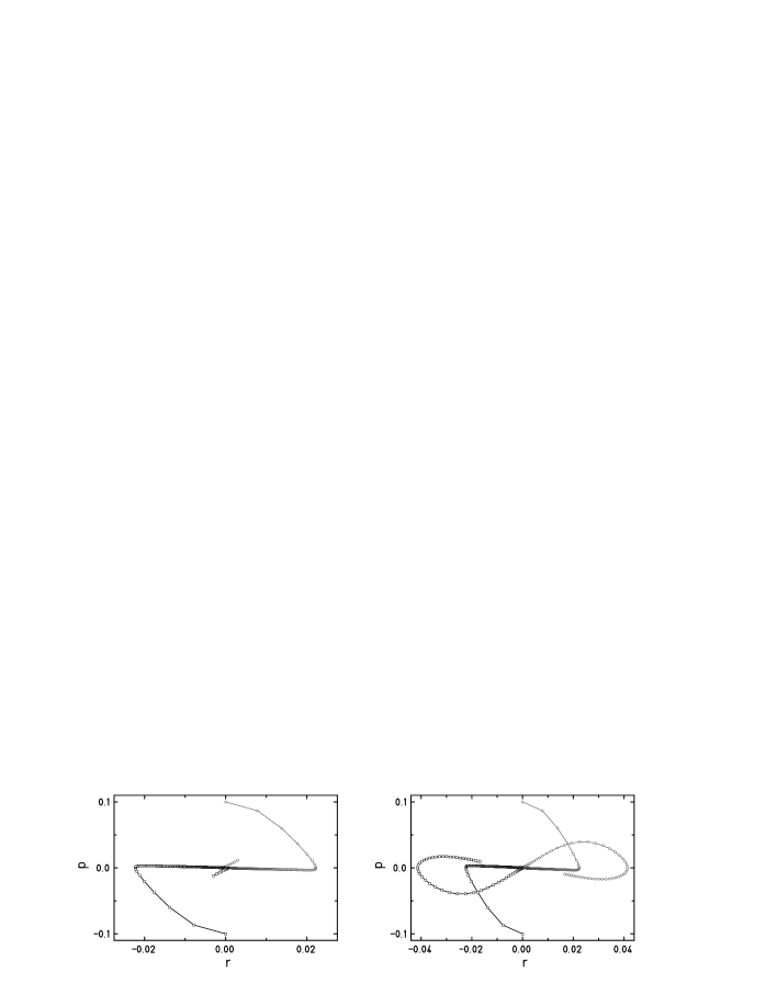
Figure 1: Left panel: isothermal dynamics of two bosons, right panel: two fermions. The initial values of $\{r_{1},p_{1},r_{2},p_{2}\}$ are $\{0,-0.1,0,0.1\}$ in both cases, the temperature is $T=0.1\hbar\omega$, and $Q_{1}=Q_{2}=0.5$. The integration time is $8.1$ periods of the harmonic oscillator for the bosons, and $6.5$ for the fermions. The time distance between the symbols is $0.013$. The figure illustrates the effect of the Bose attraction and the Pauli-blocking in the dynamics: While the bosons stay close to each other for a longer time, the fermions are immediately driven away from each other due to the exclusion principle.

In essence, the resulting effect of indistinguishability on the thermostatted dynamics of identical quantum particles looks like an attractive or repulsive interaction, although we treat a system of non-interacting particles. The interaction which is of purely statistical origin is mediated by the influence of the pseudofrictional forces. Nevertheless, one can hope that this statistical interaction influences the ergodicity of the system. As an extreme example, one could think of thermalizing only one particle and hope that the second one thermalizes due to the interaction, see next section.

3.2 Ergodicity

The classical Nosé-Hoover method applied to a single particle in a harmonic oscillator features ergodicity problems that are encountered in the quantum case, too, since the overall characteristics of the equations of motion are similar in both cases. However, there is no classical counterpart of the quantum statistical interaction between identical particles. Therefore, the question of whether the more complex equations of motion presented in the precedent section lead to improved ergodic behavior deserves attention.

For the different methods, we look at marginal distributions of the thermal weight function $f_{\varepsilon}^{(2)}$. As an example, we give the analytical expression of the marginal distribution of $r_{1}$:

$$f_{\varepsilon}(r_{1}) =\frac{1}{\tilde{Z}_{\varepsilon}^{(2)}}\int\frac{\mbox{d}p_{1}}{2\pi\hbar}\,\frac{\mbox{d}r_{2}\,\mbox{d}p_{2}}{2\pi\hbar}\;w^{(2)}_{\varepsilon}(r_{1},r_{2},p_{1},p_{2})$$ (17)

$$=\frac{1}{\tilde{Z}_{\varepsilon}^{(2)}}\sqrt{\frac{m\omega}{8\pi\hbar}}\Bigg{(}\sqrt{\frac{1}{(e^{\beta\hbar\omega}-1)^{3}}}\;e^{-\frac{m\omega}{2\hbar}(e^{\beta\hbar\omega}-1)r_{1}^{2}}$$

$$\phantom{=\frac{1}{Z_{\varepsilon}^{(2)}}\sqrt{\frac{2\pi m\omega}{\hbar}}\Bigg{(}}+\varepsilon\sqrt{\frac{1}{e^{2\beta\hbar\omega}-1}}\sqrt{\frac{1}{e^{\beta\hbar\omega}}}e^{-\frac{m\omega}{\hbar}\sinh(\beta\hbar\omega)r_{1}^{2}}\Bigg{)}\ .$$

3.2.1 Nosé-Hoover and Nosé-Hoover chain method

Figure 2: Results of time averaging with the simple Nosé-Hoover scheme for two fermions, left panel: $T=0.1$, right panel: $T=1.2$. In both cases, we used identical initial conditions, $r_{1}(0)=-r_{2}(0)=0.01$, $p_{1}(0)=-p_{2}(0)=0.01$, $p_{\eta_{1}}(0)=-p_{\eta_{2}}(0)=0.01$, $Q_{1}=Q_{2}=1.0$. We present density plots and histograms for $r_{1}$, $p_{1}$, and $p_{\eta_{1}}$; the respective results for $r_{2}$, $p_{2}$, and $p_{\eta_{2}}$ look similar.

Firstly, we present results that are obtained using the equations of motion (7), (12), i. e. the original Nosé-Hoover technique generalized to the case of two identical fermions. A detailed investigation of these equations of motion for a wide temperature range shows that the system is not ergodic in general. We find non-ergodic motion at low and intermediate temperatures $T\lesssim 1.2$. However, above that value, we find ergodic motion, and the respective marginal distributions are well matched by the histograms obtained by time averaging, see Fig. 2. This fact is to be contrasted sharply to the findings in the single-particle case, where the simple Nosé-Hoover scheme produces non-ergodic motion even at very high temperature values [2, 3].

The different behavior of the two-particle dynamics may be attributed to the statistical interaction appearing in this case. The more complicated form of the equations of motion improves the ergodicity of the scheme substantially compared to the case of a single particle.

As a result, this technique turns out to be not recommendable in the low-temperature regime. Therefore, we have investigated whether the problems of non-ergodicity can be overcome by standard methods that are known from classical molecular dynamics, e. g. with a chain of thermostats [5].

Using one additional thermostatting pseudofriction coefficient for each $p_{\eta_{i}}$, $i=1,2$, the problems of ergodicity are immediately and reliably resolved. The marginal distributions are exactly matched by the respective histograms, and the system is ergodic within the whole large temperature range that has been investigated [13]. As in the classical case, it is remarkable that a solution to the seemingly inaccessible problem of ergodicity is so easily obtained. Moreover, from the point of view of computational time, it is relatively inexpensive, since only two more degrees of freedom are added, which is negligible especially if one deals with larger systems.

We note that it is not sufficient to couple a second thermostating pseudofriction coefficient to only one parameter, say $p_{\eta_{1}}$. In this case, the marginals of $p_{\eta_{2}}$ are not sampled correctly at temperature values $T\lesssim 0.3$. Even worse, if only $p_{1}$ is coupled to a thermostat, the dynamics of the parameters $r_{2}$ and $p_{2}$ is not affected at all. Hence, the energy of particle $2$ is an additional conserved quantity, leading to strongly non-ergodic motion. This illustrates the limits of the improved ergodicity due to the statistical interaction.

3.2.2 KBB method with different coupling schemes

Figure 3: Marginal distributions obtained at $T=0.05$ with a cubic coupling scheme (left panel), and with the alternate scheme described in the text (right panel). The initial value of $\xi_{1}$ on the left panel is $\xi_{1}(0)=-5.1$, and the “freezing” of the demon variable is striking. Surprisingly, all other marginals are well reproduced. The right panel illustrates that the problem is resolved by the modified scheme.

In the original paper [6], Kusnezov, Bulgac, and Bauer propose the following choice of functions

$$g_{r_{1}}(\xi_{1})=\frac{1}{2}\xi_{1}^{2}\ ,\quad g_{r_{2}}(\xi_{2})=\frac{1}{2}\xi_{2}^{2}\ ,\quad g_{p_{1}}(\zeta_{1})=\frac{1}{4}\zeta_{1}^{4}\ ,\quad g_{p_{2}}(\zeta_{2})=\frac{1}{4}\zeta_{2}^{4}\ ,$$ (18)

as a reliable scheme that provides ergodic behavior. Using their rules of thumb for the adaptation of the respective coupling constants, we find that this cubic coupling scheme leads to ergodic motion also in the present case. However, considering the low-temperature results for fermions presented in Fig. 3, it can be inferred that the marginal distributions of the pseudofriction coefficients $\xi_{1}$, and equivalently, $\xi_{2}$ (not shown), that are linearly coupled to the system are not sampled properly in the range $T\lesssim 0.1$. The histograms presented in Fig. 3 clearly indicate that $\xi_{1}$ does not depart substantially from its initial value during the time evolution. Nevertheless, the thermal weight function $w_{\varepsilon}^{(2)}$ is sampled correctly, since all marginal distributions coincide with the exact result. However, it is obvious that the cubic coupling scheme is not ergodic in a part of the phase space at low temperatures. This applies to bosons as well.

We propose to resolve this problem by coupling the coefficents $\xi_{1}$ and $\xi_{2}$ in precisely the same manner as $\zeta_{1}$ and $\zeta_{2}$, i. e. cubically. This appears to be a sensible improvement since the distributions of $\zeta_{1}$ and $\zeta_{2}$ are sampled correctly even at very low temperatures. The resulting equations of motion yield the outcome shown in the right hand panel of Fig. 3. All marginal distributions are now sampled correctly.

3.3 Two-particle density

As an example for the determination of the canonical average of a two-particle observable, we present results of time averaging for the two-particle density,

$$\rho_{\varepsilon}^{(2)}(x_{1},x_{2})=\big{\langle}\big{\langle}\;{\frac{|\langle\,{x_{1},x_{2}}\,|\,{A_{\varepsilon}}\,\rangle|^{2}}{\langle\,{A_{\varepsilon}}\,|\,{A_{\varepsilon}}\,\rangle}}\;\big{\rangle}\big{\rangle}\ ,$$ (19)

which can also be calculated analytically. In terms of the relative and center-of-mass variables $x_{-}=\frac{1}{\sqrt{2}}(x_{1}-x_{2})$, $x_{+}=\frac{1}{\sqrt{2}}(x_{1}+x_{2})$, the result is given by

$$\rho_{\varepsilon}^{(2)}(x_{-},x_{+})=\frac{1}{\tilde{Z}_{\varepsilon}^{(2)}}\frac{m\omega}{2\pi\hbar}\frac{1}{e^{2\beta\hbar\omega}-1}\exp\left(-\frac{m\omega}{\hbar}\tanh\Big{(}{\textstyle\frac{1}{2}}\beta\hbar\omega\Big{)}(x_{+}^{2}+x_{-}^{2})\right)\\ \times\;\left(1+\varepsilon\exp\Big{(}-4\frac{m\omega}{\hbar}\frac{e^{\beta\hbar\omega}}{e^{2\beta\hbar\omega}-1}\,x_{-}^{2}\Big{)}\right)\ .$$ (20)

In order to give a useful representation of our findings, we present results of time averages along with the respective analytical results for fixed values of $x_{+}$ that have been chosen arbitrarily. Fig. 4 shows an excellent agreement.

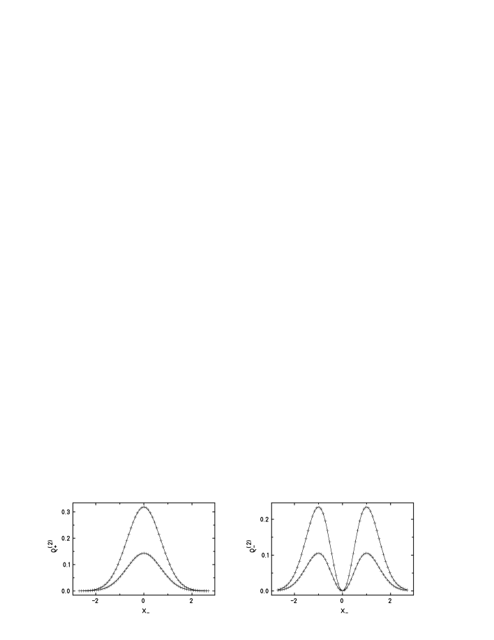
Figure 4: Results of time averages for the bosonic (left figure) and fermionic (right figure) two-particle density. The solid curves correspond to the respective analytical results as given by equation (20). In the fermionic case, the crosses are obtained from the simulations that gave the right hand panels of figure 3. The upper line corresponds to the value $x_{+}=0$, the lower line to the value $x_{+}=0.894$.

4 Summary and outlook

This article presents an extension of the powerful methods of heat bath coupling in classical MD simulations to a quantum system of identical particles. Surprisingly, the classical ansatz turns out to be suitable for the sampling of quantum entangled distribution functions. The resulting two-particle dynamics contains additional terms that act like an attractive (bosons) or repulsive (fermions) force mediated by the pseudofriction coefficients. Ergodicity problems are reliably resolved by Nosé-Hoover chains or a modification of the cubic coupling scheme, even at very low temperature values. An analytical treatment of the case of an $N$-particle Fermi system is possible, and the resulting equations are given in Ref. [13].

The most promising prospect that our method offers lies in a combination with approximate quantum dynamics schemes. A variety of such schemes is available, some of which are based on the time-dependent quantum variational principle [14] which allows to derive approximations to the time-dependent Schrödinger equation. How can we combine the thermostating method developed in this work with, e. g., Fermionic Molecular Dynamics (FMD) [9] in order to obtain an isothermal dynamical scheme for a complex interacting fermion system? Does our generalization of the classical methods to quantum dynamics permit to make the power of approximate quantum MD schemes available for the calculation of quantum canonical averages without diagonalising the full many-body Hamiltonian? This question is very timely in view of recent experiments investigating the behavior of trapped Fermi gases.

In FMD, the variational trial state is a Slater determinant of single-particle Gaussian wave packets parametrized by mean position, mean momentum, and complex width. These wave packets are frequently referred to as squeezed states and may be regarded as generalisations of coherent states. Therefore, an application of the thermostats developed in the present work to FMD appears feasible.

Another idea of combining FMD with a thermostat is to cool the system of interest “sympathetically”, i. e. via an interaction between particles that are kept at a constant temperature by a quantum Nosé-Hoover chain and the physical system under investigation. This corresponds precisely to the experimental technique of “sympathetic cooling” currently employed to investigate ultracold fermionic gases [15, 16]. Since the thermalizing of the particles coupled to a Nosé-Hoover chain would correspond to a thermalizing of non-interacting particles, such a method is only approximately correct since we need to employ an interaction to enable the sympathetic cooling.

Despite these difficulties, an important asset of an isothermal MD scheme is that it can possibly provide temporal information, in particular time correlation functions. Although it is not clear to which degree the extended system methods realistically mimic the heat bath interaction, the underlying equations of motion are physically reasonable. Therefore, in principle, this method is tailor-made to model the particle dynamics at constant temperature in a magnetic trap.

Acknowledgments
The authors would like to thank the Deutsche Forschungsgemeinschaft (DFG) for financial support of the project “Isothermal dynamics of small quantum systems”.

References

• [1] M. E. Tuckerman, G. J. Martyna, J. Phys. Chem. B 104 (2000) 159
• [2] D. Mentrup, J. Schnack, Physica A 297 (2001) 337
• [3] W. G. Hoover, Phys. Rev. A31 (1985) 1685
• [4] S. Nosé, Prog. Theor. Phys. Suppl. 103 (1991) 1
• [5] G. J. Martyna, M. L. Klein, M. Tuckerman, J. Chem. Phys. 97 (1992) 2635
• [6] D. Kusnezov, A. Bulgac, W. Bauer, Ann. of Phys. 204 (1990) 155
• [7] M. Grilli, E. Tosatti, Phys. Rev. Lett. 62 (1989) 2889
• [8] D. Kusnezov, Phys. Lett. A184 (1993) 50
• [9] H. Feldmeier, J. Schnack, Rev. Mod. Phys. 72 (2000) 655
• [10] J. R. Klauder, B.-S. Skagerstam, Coherent states, World Scientific Publishing, Singapore 1985
• [11] J. Schnack, PhD thesis, TH Darmstadt, 1996
• [12] J. Schnack, Europhys. Lett. 45 (1999) 647
• [13] D. Mentrup, PhD thesis, Universität Osnabrück, 2003
• [14] P. Kramer, M. Saraceno, Geometry of the Time-Dependent Variational Principle in Quantum Mechanics, Lecture Notes in Physics 140, Springer, Berlin (1981)
• [15] C. J. Myatt, E. A. Burt, R. W. Ghrist, E. A. Cornell, and C. E. Wieman, Phys. Rev. Lett 78 (1997) 586
• [16] B. DeMarco, D. S. Jin, Phys. Rev. A 58 (1998) R4267