Dynamics and thermodynamics of the
spherical frustrated Blume-Emery-Griffiths model

Abstract

We introduce a spherical version of the frustrated Blume-Emery-Griffiths model and solve exactly the statics and the Langevin dynamics for zero particle-particle interaction $\left(K=0\right)$. In this case the model exhibits an equilibrium transition from a disordered to a spin glass phase which is always continuous for nonzero temperature. The same phase diagram results from the study of the dynamics. Furthermore, we notice the existence of a nonequilibrium time regime in a region of the disordered phase, characterized by aging as occurs in the glassy phase. Due to a finite equilibration time, the system displays in this region the pattern of interrupted aging.

PACS numbers: 05.50.+q, 64.70.Pf, 75.10.Nr, 64.60.Ht

I Introduction

Many important features of spin glass models at mean field level have come out by studying their relaxional Langevin dynamics from a random initial condition[1, 2, 3, 4, 5, 6, 7, 8, 9]. The structure of the dynamical equations for the correlation and response functions has reaveled some analogies with other types of complex systems in which the disorder is apriori absent: at equilibrium the dynamics becomes formally identical to the Mode Coupling Theory (MCT), which is the main approach to the supercooled liquids near the glass structural transition [10]. Thus there have been strong feelings that the two types of systems are deeply connected; in the glasses an effective disorder is self-induced by the slow dynamics of the microscopical variables [2].

For spin glass systems, the dynamical equations have been studied also in the low temperature phase [5, 6, 7, 8, 9]. These works provide a suggestion to extend the MCT below the glass temperature [11]. One of the main result has been that for these temperatures the system never reaches the equilibrium, but rather displays an off-equilibrium behaviour where the dynamics depends on the whole history of the system up to the beginning of its observation and is characterized by the loss of validity of typical equilibrium properties, as the time traslational invariance (TTI) and the fluctuation-dissipation theorem (FDT). One can thus establish contact with some nonequilibrium experimental observations, namely the slow relaxations and the aging phenomena which are observed for real spin glasses and many other complex systems [9].

Despite the cited resemblance, spin glasses are microscopically quite different from liquids and thus not suitable to their description. Recently, to make stronger connections with liquids, some models have been introduced which combine features of spin glasses and lattice gas. Being constituted of particles, they allow to introduce the density and other related quantities which are usually important in the study of liquids. In this regard we consider the frustrated Blume-Emery-Griffiths (BEG) model [17, 18], which is a quite general framework to describe different glassy systems. Its mean field hamiltonian is:

$$H=-\sum_{i<j}J_{ij}s_{i}n_{i}s_{j}n_{j}-\frac{K}{N}\sum_{i<j}n_{i}n_{j}-\mu\sum_{i}n_{i}$$ (1)

where $s_{i}=\pm 1$, $n_{i}=0,1$, $\mu$ is the chemical potential and $J_{ij}$ are quenched gaussian interactions having zero mean and variance $\left[J_{ij}^{2}\right]_{J}=1/N$ [21]. Essentially the model consists of a lattice gas in a frustrated medium where the particles have an internal degree of freedom, given by their spin, which may account, as an example, of the possible orientations of complex molecules in glass forming systems. These steric effects are indeed greatly responsible for the geometric frustration appearing in glass forming systems at low temperatures or high densities. Besides that, the particles interact through a potential depending on the coupling $K$. In particular for $K=0$ one recovers the Ghatak-Sherrington model [13] and for $K=-1$ the Ising Frustrated Lattice Gas model [14]; this last case is related to the problem of the site frustrated percolation [15] and has been also used in the presence of gravity to describe granular materials [16]. However, as found by standard replica theory [17, 18], the model does not display substantial differences by varying $K$. The phase diagram in the plane $\mu-T$ shows a critical line separating a spin glass phase from a disordered one; the transition is continuous for large $\mu$, as for the standard Ising spin glass ($n_{i}=1$), up to a given value $\mu^{*}_{K}$ below which becomes discontinuous; in this region the Parisi solution has been obtained only recently in [18]. Moreover, we note that a dynamical treatment of the model is still lacking.

We propose a spherical version of the frustrated BEG model which allows a complete analysis of its equilibrium properties and even of Langevin dynamics. In this paper we study this model for $K=0$ leaving the general case to future investigations [20]. We find an equilibrium transition to a spin glass phase for $\mu\geq-1$, which is always continuous, like in the spherical SK model [12], except for $\mu=-1$ and $T=0$ (see Fig. 1). Furthermore, we investigate the Langevin dynamics of the various two-time functions and of density in the whole phase diagram. We get exact expressions of these quantities that are in general rather complex; they depend on several characteristic time scales whose number changes in the various regions of the phase diagram. In particular, the largest of these times is found to represent the charactristic equilibration time of the system, $\tau_{eq}$. In the nonglassy phase this is finite and for waiting times $t^{\prime}>\tau_{eq}$ the two-time functions obey TTI and FDT. This is no more true for $t^{\prime}<\tau_{eq}$, the system being still out of equilibrium. By studying this regime near the critical line where $\tau_{eq}$ is large, we find two different behaviours of the systems for $\mu>-1$ and $\mu\simeq-1$. We give here a first qualitative description of them. In the case $\mu>-1$ FDT still holds for $t-t^{\prime}\ll t^{\prime}$, so that deviations from the equilibrium case occur only for very small values of the correlation. Instead, as $\mu$ is close to $-1$, the range of correlation values in the FDT regime decreases and for $\mu=-1$ this vanishes; if $t,t^{\prime}$ are sufficiently lower than $\tau_{eq}$ the correlation function scales as a power of $t^{\prime}/t$. Thus, in this region the observation of the system over short time scales could wrongly lead to conclude that the system is in the glassy phase. Then, for a large but finite $\tau_{eq}$, the model follows the pattern of interrupted aging. Finally, $\tau_{eq}$ diverges in the whole glassy phase and the system displays essentially the same nonequilibrium behaviour of the spherical SK model [7].

The paper is organized as follows. In Sec. II we define the spherical frustrated BEG model. In Sec. III we deal with the statics using the theory of large random matrices and analyse the thermodynamical properties. In Sec. IV we introduce the Langevin dynamical model and the various quantities of interest. In Sec. V we solve the integral equation related to the spherical constraints and compute the density. In Sec. VI we discuss the dynamics in the disordered phase and, after the identification of the equilibration time $\tau_{eq}$, we analyse the equilibrium regime $\left(t^{\prime}>\tau_{eq}\right)$ and the out of equilibrium one $\left(t^{\prime}<\tau_{eq}\right)$. In Sec. VII we consider the nonequilibrium dynamics in the glassy phase $\left(\tau_{eq}=\infty\right)$. Finally, in Sec. VIII we present some conclusions. Furthermore, in the App. A and B we study in detail respectively the equilibrium saddle point equation and the dynamics when this equation has degenere roots.

II Definition of the model

First of all we note that the hamiltonian (1) can be rewritten in terms of two new Ising spin fields $s_{1i},s_{2i}=\pm 1$:

$$H=-\sum_{i<j}\frac{J_{ij}}{4}\left(s_{1i}+s_{2i}\right)\left(s_{1j}+s_{2j}\right)-\frac{K}{4N}\sum_{i<j}\left(s_{1i}s_{2i}+1\right)\left(s_{1j}s_{2j}+1\right)-\frac{\mu}{2}\sum_{i}\left(s_{1i}s_{2i}+1\right)$$ (2)

where:

$$\left\{\begin{array}[]{l}s_{1i}=s_{i}\\ s_{2i}=s_{i}\left(2n_{i}-1\right)\end{array}\right.\quad\Leftrightarrow\quad\left\{\begin{array}[]{l}s_{i}=s_{1i}\\ n_{i}=\frac{1}{2}\left(s_{1i}s_{2i}+1\right)\end{array}\right.$$ (3)

[21]. The 4-fields interaction in (1) is replaced in (2) by four double field interactions; furthermore the hamiltonian (2) is symmetric under the exchange of the two spin fields. The overlap $q=\left[\left\langle s_{i}n_{i}\right\rangle^{2}\right]_{J}$ and the density $d=\left[\left\langle n_{i}\right\rangle\right]_{J}$, which are two usual order parameters for a diluted spin glass, now become respectively $\frac{1}{4}\left[\left\langle s_{1i}+s_{2i}\right\rangle^{2}\right]_{J}$ and $\frac{1}{2}\left[\left\langle s_{1i}s_{2i}\right\rangle+1\right]_{J}$. So far we have just reformulated the BEG model. Now to define our spherical version let the Ising constraints fall in (2) and replace them by the spherical ones: $\sum_{i}s_{1i}^{2}=\sum_{i}s_{2i}^{2}=N$. This particular choice of the variables to sphericize aims to obtain an exactly solvable model. It recovers the spherical SK model [12] in the large $\mu$-limit ($s_{1i}=s_{2i}$). Below we’ll consider the case $K=0$.

To study the model it is convenient to diagonalize the interaction matrix $J_{ij}$ ($\sum_{j}J_{ij}\eta_{j\lambda}=\lambda\eta_{i\lambda}$) and work with the variables $s_{a\lambda}=\sum_{i}\eta_{i\lambda}s_{ai}\quad(a=1,2)$; these obey the properties $\sum_{i}s_{ai}s_{bi}=\sum_{\lambda}s_{a\lambda}s_{b\lambda}$ and $\sum_{ij}J_{ij}s_{ai}s_{bj}=\sum_{\lambda}\lambda s_{a\lambda}s_{b\lambda}$. In the $N\rightarrow\infty$ limit the eigenvalue density $\rho\left(\lambda\right)$ satisfies the Wigner semi-circle law:

$$\rho\left(\lambda\right)=\left\{\begin{array}[]{ll}\frac{1}{2\pi}\sqrt{4-\lambda^{2}}&\left|\lambda\right|<2\\ 0&\left|\lambda\right|\geq 2\end{array}\right.$$ (4)

the quantities $\eta_{i\lambda}$ are gaussian variables with zero mean and moments $\left[\eta_{i\lambda}^{2k}\right]_{J}=\frac{\left(2k-1\right)!!}{N^{k}}$; they are uncorrelated to the eigenvalues and among themselves apart the orthonormality and closure conditions.

III Equilibrium properties

A Saddle point equation

The statics can be solved by standard techniques for spherical models and the above properties of large random matrices [12]. In the $N\rightarrow\infty$ limit the free energy is evaluated by steepest descent, by imposing saddle point conditions with respect to the two Lagrange multipliers $z_{1}$ and $z_{2}$, introduced by the spherical constraints. These equations just reproduce the two constraints satisfied on average, $\sum_{\lambda}\left\langle s_{a\lambda}^{2}\right\rangle=N\quad(a=1,2)$. Explicitly they are reduced to the only one:

$$\frac{1}{2\beta^{2}}\left[z-\sqrt{z^{2}-4\beta^{2}}\right]=1-\frac{1}{z+2\beta\mu}$$ (5)

where $z=z_{1}+\beta\mu=z_{2}+\beta\mu$ has to be greater than the two branch points $\left\{2\beta,-2\beta\mu\right\}$. This condition is satisfied by a unique solution of (5), denoted by $z_{s}$, for each $T$ if $\mu<-1$ and above a critical line, $T=T_{c}\left(\mu\right)$, for $\mu\geq-1$. This region of the phase diagram identifies the disordered phase (labelled by P in Fig. 1). The critical line is located by $z_{s}$ reaching the branch point $2\beta$ and is given by:

$$T_{c}\left(\mu\right)=\frac{\mu+1}{\mu+3/2}$$ (6)

A detailed study of Eq. (5) is given in App. A. Below the critical line (phase SG in Fig. 1) this equation is not satisfied for $z>2\beta$. The equilibrium saddle value of $z$ sticks at the branch point $2\beta$, and to preserve the spherical constraints a spontaneous magnetization arises along the eigenvector with eigenvalue $2$. Actually, the diluted overlap $q=\frac{1}{4}\left[\left\langle s_{1i}+s_{2i}\right\rangle^{2}\right]_{J}$ is found to vanish when Eq. (5) holds and becomes just $\frac{\left\langle s_{a,\lambda=2}\right\rangle^{2}}{N}$ below the critical line, i.e.:

$$q=1-\frac{1}{\beta}-\frac{1}{2\left(\beta+\beta\mu\right)}=1-\frac{T}{T_{c}\left(\mu\right)}$$ (7)

The transition at the line $T=T_{c}\left(\mu\right)$ is continuous for each $\mu>-1$ and discontinuous in the point $(\mu=-1,T=0)$. Indeed the zero temperature value of $q$ is $\vartheta\left(\mu+1\right)$ with $q=0$ for $\mu=-1$.

Note that model could be solved using the replica trick, where a replica symmetric ansatz yields identical results.

FIG. 1.: The phase diagram $T$ vs. $\mu$. The critical line separating the two phases is given by Eq. (6) for $\mu\geq-1$. The transition is always continuous except for the point $\left(\mu=-1,T=0\right)$.

B Free energy and related quantities

The free energy per site $f$ can be explicitly evaluated:

$$\beta f=\left\{\begin{array}[]{ll}-\frac{z_{s}+2\beta\mu}{2}-\ln 4\pi+\frac{1}{2}\ln\left(z_{s}+2\beta\mu\right)+\frac{\beta^{2}}{4}\left(1-\frac{1}{z_{s}+2\beta\mu}\right)^{2}-\frac{1}{2}\ln\left(1-\frac{1}{z_{s}+2\beta\mu}\right)&P\\ -\left(\beta+\beta\mu\right)-\ln 4\pi+\frac{1}{2}\ln 2\left(\beta+\beta\mu\right)+\frac{1}{4}+\frac{1}{2}\ln\beta&SG\end{array}\right.$$ (8)

it corresponds to a negative low temperature entropy which diverges logarithmically as $T\rightarrow 0$. This pathology is typical of spherical models, even in the short-ranged uniform case.

Now we analyse other thermodynamic quantities in order to characterize the system and for comparison with the Ising case [17, 18]. The density $d=\frac{1}{2}\left[\left\langle s_{1i}s_{2i}\right\rangle+1\right]_{J}$ is given by $-\frac{\partial f}{\partial\mu}$:

$$d=\left\{\begin{array}[]{ll}1-\frac{1}{z_{s}+2\beta\mu}&P\\ 1-\frac{1}{2\left(\beta+\beta\mu\right)}&SG\end{array}\right.$$ (9)

it is represented in Fig. 2 as a function of $T$ for several values of $\mu$. In the large temperature limit $d$ approaches the value $1/2$ for each $\mu$. For $T=0$ we get $d=q=\vartheta\left(\mu+1\right)$ with $d=q=0$ for $\mu=-1$; note that, unlike the Ising version, there is no interval of $\mu$ values where $0<d<1$. In the spin glass phase a partial freezing takes place ($d<q<1$), except at zero temperature where the system is fully frozen ($d=q=1$). For $\mu\rightarrow\infty$ the model approaches the spherical SK limit [12]: $T_{c}=1$, $d=1$, $q=1-T$.

FIG. 2.: The density $d$ vs. $T$ for several values of $\mu$. The intersection of the curves with the dotted line locates the critical temperature $T_{c}\left(\mu\right)$. Thus, the initial straight part of the curves for $\mu>-1$ corresponds to temperatures for which the system is in the glassy phase (bottom of Eq. (9)). In the large $T$ limit $d$ goes to the value $1/2$ for each $\mu$. Note also that at zero temperature $d=1$ for $\mu>-1$ and $d=0$ for $\mu\leq-1$.

The compressibility $k=\frac{1}{\beta}\frac{\partial d}{\partial\mu}$ is found to be:

$$k=\left\{\begin{array}[]{ll}\frac{2\left(1-\frac{1}{z_{s}+2\beta\mu}\right)}{\left(z_{s}+2\beta\mu\right)^{2}\left(1-\frac{1}{z_{s}+2\beta\mu}\right)+\sqrt{z_{s}^{2}-4\beta^{2}}}&P\\ \frac{1}{2\left(\beta+\beta\mu\right)^{2}}&SG\end{array}\right.$$ (10)

its plot as a function of $T$ is given in Fig. 3. It’s evident a cusp at the critical temperature $T_{c}\left(\mu\right)$ whose height diverges in the limit $\mu\rightarrow-1^{+}$. $k$ goes to the value $1/4$ for each $\mu$ in the large temperature limit. For zero temperature $k=0$ for each $\mu$.

FIG. 3.: The compressibility $k$ vs. $T$ for several values of $\mu$. A cusp is evident at the critical temperature $T_{c}\left(\mu\right)$ at least for values of $\mu$ close to $-1$. The height of the cusp diverges as $\mu\rightarrow-1^{+}$. The intersection of the dotted line with the curves for $\mu>-1$ locates the critical temperature $T_{c}\left(\mu\right)$; $k$ increases with the square of $T$ in the glassy phase (bottom of Eq. (10)). For $T\rightarrow\infty$ $k$ goes to $1/4$ for each $\mu$.

Finally the specific heat $c$ is:

$$c=\left\{\begin{array}[]{ll}1-\frac{z_{s}}{2}-\frac{\sqrt{z_{s}^{2}-4\beta^{2}}\left[\left(z_{s}+2\beta\mu\right)^{2}\left(1-\frac{1}{z_{s}+2\beta\mu}\right)+\beta\mu\right]-\left(z_{s}+2\beta\mu\right)^{2}}{\left(z_{s}+2\beta\mu\right)^{2}\left(1-\frac{1}{z_{s}+2\beta\mu}\right)+\sqrt{z_{s}^{2}-4\beta^{2}}}&P\\ 1&SG\end{array}\right.$$ (11)

it presents a cusp at the transition for $\mu>-1$, while for $T=0$ is discontinuous since $c=\frac{1}{2}$ for $\mu\leq-1$ (Fig. 4). The large $\mu$ limit is given by $c=\frac{1}{2}+\frac{1}{2T^{2}}$ for $T>1$.

FIG. 4.: The specific heat $c$ vs. $T$ for several values of $\mu$. Note the cusp at the transition temperature $T_{c}\left(\mu\right)$ for $\mu>-1$. $c=1$ in the glassy phase (bottom of Eq. (11)). In the zero $T$ limit $c=1/2$ for each $\mu\leq-1$.

C In the presence of a magnetic field

Adding to the hamiltonian (2) a magnetic field term, $-\sum_{i}\frac{h_{i}}{2}\left(s_{1i}+s_{2i}\right)$, the saddle point equation is modified by adding $\int d\lambda\rho\left(\lambda\right)\frac{\left(\beta h_{\lambda}\right)^{2}}{\left(z-\beta\lambda\right)^{2}}$ to the left hand side of Eq. (5). Assuming a uniform field, $h_{i}=h$, one can replace $h_{\lambda}^{2}$ by its average value $h^{2}$. Thus one finds that for $h\neq 0$ there is no transition, since in this case $z_{s}$ never reaches the branch point $2\beta$.

Let us now compute the diluted susceptibilitise in zero field. The linear one obeys the diluted Curie law in the disordered phase and is constant for $T<T_{c}\left(\mu\right)$, so to display a cusp crossing the critical line (Fig. 5):

$$\chi=\left.-\frac{\partial^{2}f}{\partial h^{2}}\right|_{h=0}=\left\{\begin{array}[]{ll}\beta\left(1-\frac{1}{z_{s}+2\beta\mu}\right)&P\\ 1&SG\end{array}\right.$$ (12)

notice that the previous result can be obtained also from the linear response theorem $\chi=\beta\left(d-q\right)$. The zero temperature expression is $\chi=-\mu-\sqrt{\mu^{2}-1}$ for $\mu\leq-1$.

FIG. 5.: The susceptibility $\chi$ vs. $T$ for several values of $\mu$. Note the cusp at the transition temperature $T_{c}\left(\mu\right)$ for $\mu>-1$. $\chi=1$ in the glassy phase (bottom of Eq. (12)). In the zero $T$ limit $\chi=-\mu-\sqrt{\mu^{2}-1}$ for $\mu\leq-1$.

The spin glass susceptibility is given by:

$$\chi_{SG}=\sum_{\lambda\mu}\left(\frac{\partial^{2}f}{\partial h_{\lambda}\partial h_{\mu}}\right)_{h=0}^{2}=\left\{\begin{array}[]{ll}\frac{1}{2}\left(\frac{z_{s}}{\sqrt{z_{s}^{2}-4\beta^{2}}}-1\right)&P\\ \infty&SG\end{array}\right.$$ (13)

coming from high temperatures it diverges at the critical line as $\frac{1}{T-T_{c}\left(\mu\right)}$ and remains infinite in the whole frozen phase. For zero temperature it is given by $\chi_{SG}=\frac{1}{2}\left(-\frac{\mu}{\sqrt{\mu^{2}-1}}-1\right)$ for $\mu\leq-1$. The large $\mu$ limit is $\chi_{SG}=\frac{1}{T^{2}-1}$ for $T>1$.

IV Langevin dynamics

Now we deal with the Langevin relaxional dynamics of the model. Let us assume that the two spin fields evolve via usual Langevin equations, which when projected onto the basis $\lambda$ become:

$$\left\{\begin{array}[]{c}\frac{ds_{1\lambda}}{dt}=\left(\frac{\lambda}{4}-\frac{z_{1}\left(t\right)}{2}\right)s_{1\lambda}+\left(\frac{\lambda}{4}+\frac{\mu}{2}\right)s_{2\lambda}+h_{1\lambda}\left(t\right)+\xi_{1\lambda}\left(t\right)\\ \frac{ds_{2\lambda}}{dt}=\left(\frac{\lambda}{4}+\frac{\mu}{2}\right)s_{1\lambda}+\left(\frac{\lambda}{4}-\frac{z_{2}\left(t\right)}{2}\right)s_{2\lambda}+h_{2\lambda}\left(t\right)+\xi_{2\lambda}\left(t\right)\end{array}\right.$$ (14)

where $z_{a}\left(t\right)\ \ a=1,2$ are two time-dependent Lagrange multipliers enforcing the spherical constraints, $h_{a\lambda}\left(t\right)$ two external fields interacting with the field $s_{a\lambda}$ and $\xi_{a\lambda}$ the thermal noises with zero mean and correlations $\left\langle\xi_{a\lambda}\left(t\right)\xi_{b\mu}\left(t^{\prime}\right)\right\rangle=2T\delta_{ab}\delta_{\lambda\mu}\delta\left(t-t^{\prime}\right)\ \ a,b=1,2$. Hereafter we use $\left\langle\text{ }\right\rangle$ to represent the average over the thermal noises.

Let us now introduce the quantities of interest, namely the correlation functions $C_{ab}\left(t,t^{\prime}\right)$ $\left(a,b=1,2\right)$, the response functions $G_{ab}\left(t,t^{\prime}\right)$ and the density $d\left(t\right)$:

$$C_{ab}\left(t,t^{\prime}\right) = \left[\frac{1}{N}\sum_{i}\left\langle s_{ai}\left(t\right)s_{bi}\left(t^{\prime}\right)\right\rangle\right]_{J}=\int d\lambda\,\rho\left(\lambda\right)\left\langle s_{a\lambda}\left(t\right)s_{b\lambda}\left(t^{\prime}\right)\right\rangle$$ (15)

$$G_{ab}\left(t,t^{\prime}\right) = \left[\frac{1}{N}\sum_{i}\left.\frac{\delta\left\langle s_{ai}\left(t\right)\right\rangle}{\delta h_{bi}\left(t^{\prime}\right)}\right|_{h=0}\right]_{J}=\int d\lambda\,\rho\left(\lambda\right)\left.\frac{\delta\left\langle s_{a\lambda}\left(t\right)\right\rangle}{\delta h_{b\lambda}\left(t^{\prime}\right)}\right|_{h=0}$$ (16)

$$d\left(t\right) = \frac{1}{2}\left(C_{12}\left(t,t\right)+1\right)$$ (17)

A quite general procedure allows to derive from (14) closed equations for these functions as saddle point solutions of a dynamical generating functional [1, 2]. Using this procedure one implicitely assumes the initial lattice fields $s_{ai}\left(0\right)$ as random variables with a gaussian distribution of zero mean and variance $\overline{s_{ai}\left(0\right)s_{bi}\left(0\right)}=1+2\left(1-\delta_{ab}\right)\left(d\left(0\right)-1\right)$ (the overbar stands for the average over the random initial conditions); the same is valid for $s_{a\lambda}\left(0\right)$, since the rotational invariance of the gaussian distribution. However, in our case these functional techniques can be avoided, as much as [3, 7]. Due to its linearity, the Langevin system (14) can be explicitely solved for given noises, thus the various dynamical quantities can be evaluated averaging over the noises and the eigenvalues $\lambda$. In the following we choose the initial conditions indicated previously. The dynamical model can be solved for any $d\left(0\right)$; but it can be shown that the value of $d\left(0\right)$ does not influence the long time behaviour for nonzero temperatures, so we’ll take for simplicity $d\left(0\right)=1$.

For zero external fields the dynamical model is for each time symmetric under the exchange of the two spin fields. Since below we’ll discuss the dynamics only in this case, we can exploit this symmetry and limit ourselves to solve Eqs. (14) for $z_{1}\left(t\right)=z_{2}\left(t\right)$. The solution is then given by:

$$s_{a\lambda}\left(t\right) = \frac{1}{2\sqrt{\Gamma\left(t\right)}}\left\{e^{\lambda t/2}\left[s_{1\lambda}\left(0\right)+s_{2\lambda}\left(0\right)\right]+\eta_{a}e^{-\mu t}\left[s_{1\lambda}\left(0\right)-s_{2\lambda}\left(0\right)\right]\right.$$ (20)

$$+\int_{0}^{t}du\,e^{\lambda\left(t-u\right)/2}\sqrt{\Gamma\left(u\right)}\left[\xi_{1\lambda}\left(u\right)+h_{1\lambda}\left(u\right)+\xi_{2\lambda}\left(u\right)+h_{2\lambda}\left(u\right)\right]$$

$$\left.+\eta_{a}\int_{0}^{t}du\,e^{-\mu\left(t-u\right)}\sqrt{\Gamma\left(u\right)}\left[\xi_{1\lambda}\left(u\right)+h_{1\lambda}\left(u\right)-\xi_{2\lambda}\left(u\right)-h_{2\lambda}\left(u\right)\right]\right\}$$

where $\eta_{a}=\delta_{a,1}-\delta_{a,2}$ and

$$\Gamma\left(t\right)=\exp\int_{0}^{t}z\left(u\right)du\qquad z\left(t\right)=z_{1}\left(t\right)-\mu=z_{2}\left(t\right)-\mu$$ (21)

As a consequence of the above symmetry, in the absence of external fields the four correlation functions coincide mutually, so we have to study only two of them: $C_{1a}\;\left(a=1,2\right)$. The same occurs for the relative response functions. Notice that, when written in the original variables $s_{i}$ and $n_{i}$, $C_{11}\left(t,t^{\prime}\right)$ is just the spin-spin correlation function, while $C_{12}\left(t,t^{\prime}\right)$ is a rather strange correlator made by a combination of spin and density variables. Instead, the density-density connected correlation function, which enters in the schematic version of MCT [22], involves 4-spin functions in the formalism of the lattice fields $s_{1},s_{2}$:

$$C_{nn}\left(t,t^{\prime}\right)=\left[\frac{1}{4N}\sum_{i}\left[\left\langle s_{1i}\left(t\right)s_{2i}\left(t\right)s_{1i}\left(t^{\prime}\right)s_{2i}\left(t^{\prime}\right)\right\rangle-\left\langle s_{1i}\left(t\right)s_{2i}\left(t\right)\right\rangle\left\langle s_{1i}\left(t^{\prime}\right)s_{2i}\left(t^{\prime}\right)\right\rangle\right]\,\right]_{J}$$ (22)

However, since the model is quadratic, this quantity is readily related to $C_{1a}$ and we get $C_{nn}\left(t,t^{\prime}\right)=\frac{1}{4}\left[C_{11}\left(t,t^{\prime}\right)^{2}+C_{12}\left(t,t^{\prime}\right)^{2}\right]$.

From Eq. (20), taking into account of the previous initial conditions, we find for $t\geq t^{\prime}$ and zero external fields:

$$C_{1a}\left(t,t^{\prime}\right) = \frac{2}{\sqrt{\Gamma\left(t\right)\Gamma\left(t^{\prime}\right)}}\left[\frac{I_{1}\left(t+t^{\prime}\right)}{t+t^{\prime}}+T\int_{0}^{t^{\prime}}du\left(\frac{I_{1}\left(t+t^{\prime}-2u\right)}{t+t^{\prime}-2u}+\frac{\eta_{a}e^{-\mu\left(t+t^{\prime}-2u\right)}}{2}\right)\Gamma\left(u\right)\right]$$ (24)

$$G_{1a}\left(t,t^{\prime}\right) = \sqrt{\frac{\Gamma\left(t^{\prime}\right)}{\Gamma\left(t\right)}}\left[\frac{I_{1}\left(t-t^{\prime}\right)}{t-t^{\prime}}+\frac{\eta_{a}}{2}e^{-\mu\left(t-t^{\prime}\right)}\right]$$ (25)

In these formulas $I_{1}$ is the modified Bessel function of order $1$; we have used that $\int d\lambda\rho\left(\lambda\right)e^{\lambda t}=\frac{I_{1}\left(2t\right)}{t}$. Instead, the function $\Gamma\left(t\right)$ is still indeterminate; it can be computed self-consistently, as solution of the integral equation obtained by enforcing the spherical constraint $C_{11}\left(t,t\right)=1$:

$$\Gamma\left(t\right)=\frac{I_{1}\left(2t\right)}{t}+T\int_{0}^{t}du\left[\frac{I_{1}\left(2\left(t-u\right)\right)}{t-u}+e^{-2\mu\left(t-u\right)}\right]\Gamma\left(u\right)$$ (26)

Taking into account of Eq. (26), one can get the following useful expressions for $C_{1a}\left(t,t^{\prime}\right)$ and $d\left(t\right)$:

$$C_{1a}\left(t,t^{\prime}\right) = \frac{\Gamma\left(\frac{t+t^{\prime}}{2}\right)}{\sqrt{\Gamma\left(t\right)\Gamma\left(t^{\prime}\right)}}\left\{1+2\delta_{a,2}\left[d\left(\frac{t+t^{\prime}}{2}\right)-1\right]\right.$$ (29)

$$\left.-2T\int_{t^{\prime}}^{\left(t+t^{\prime}\right)/2}du\left[\frac{I_{1}\left(t+t^{\prime}-2u\right)}{t+t^{\prime}-2u}+\frac{\eta_{a}}{2}e^{-\mu\left(t+t^{\prime}-2u\right)}\right]\frac{\Gamma\left(u\right)}{\Gamma\left(\frac{t+t^{\prime}}{2}\right)}\right\}$$

$$d\left(t\right) = 1-\frac{T}{\Gamma\left(t\right)}\int_{0}^{t}due^{-2\mu\left(t-u\right)}\Gamma\left(u\right)$$ (30)

We note from these formulas that the behaviour of $C_{1a}\left(t,t^{\prime}\right)$ at large times can be deduced from that of $\Gamma$ and $d$; instead $d\left(t\right)$ takes contributions from $\Gamma$ also at low times. However we will able to compute exactly $\Gamma\left(t\right)$ for each time and then also $d\left(t\right)$. In the limit $\mu\rightarrow\infty$ one can neglect the last term in Eqs. (24),…,(30); hence $d\left(t\right)=1$, the two correlation functions and the two response functions coincide, recovering the case of spherical SK model [7].

V Computing the function $\Gamma$ and the density

Firstly, we get $\Gamma\left(t\right)$ solving the integral equation (26) by Laplace transform techniques. Following [7], one could solve Eq. (26) using a suitable expansion which is valid in the spin glass phase. However, we proceed by a different technique in order to obtain $\Gamma\left(t\right)$ in the whole phase diagram. We find that the structure of the function $\Gamma\left(t\right)$ is related to the general roots of Eq. (5), discussed in all details in App. A.

Taking the Laplace transform of Eq. (26) and using the convolution theorem, after some algebra we put $\Gamma\left(s\right)$ in the form:

$$\Gamma\left(s\right)=\beta\left[\frac{P\left(\beta s\right)}{C\left(\beta s\right)}-\beta\frac{Q\left(\beta s\right)}{C\left(\beta s\right)}\left(\frac{s-\sqrt{s^{2}-4}}{2}\right)\right]$$ (31)

where $P\left(z\right)=\left(z+2\beta\mu\right)^{2}$, $Q\left(z\right)=\left(z+2\beta\mu\right)\left(z+2\beta\mu-1\right)$ and $C\left(z\right)$ is a third degree polynomial given by Eq. (A2). We see that $\Gamma\left(s\right)$ is written in terms of rational functions and $\frac{s-\sqrt{s^{2}-4}}{2}$ which is the Laplace transform of $\frac{I_{1}\left(2t\right)}{t}$; thus in this form we can take readily the inverse transform. If $C\left(z\right)$ has distinct roots $a_{k}$ $\left(k=1,2,3\right)$ this is given by:

$$\Gamma\left(t\right)=\sum_{k=1}^{3}\left[\phi_{k}^{P}\left(a_{k}\right)e^{\left(a_{k}/\beta\right)t}-\beta\phi_{k}^{Q}\left(a_{k}\right)\int_{0}^{t}e^{\left(a_{k}/\beta\right)\left(t-u\right)}\frac{I_{1}\left(2u\right)}{u}du\right]$$ (32)

where $\phi_{k}^{P}\left(a_{k}\right)=\frac{P\left(a_{k}\right)}{C^{\prime}\left(a_{k}\right)}$ and $\phi_{k}^{Q}\left(a_{k}\right)=\frac{Q\left(a_{k}\right)}{C^{\prime}\left(a_{k}\right)}$ with $k=1,2,3$. The case of degenere roots (lines $l_{i}$ in Fig. 8) can be treated analogously and presents no qualitative differences; so we leave it in App. B.

The integral appearing in Eq. (32) can be manipulated using the integral representation of the modified Bessel function $I_{1}$; we obtain

$$\int_{0}^{t}e^{-c\omega}\frac{I_{1}\left(\omega\right)}{\omega}d\omega=c-\sqrt{c^{2}-1}-e^{-\left(c-1\right)t}J_{c}\left(t\right),\qquad J_{c}\left(t\right)=\frac{1}{\pi}\int_{-1}^{1}dx\frac{\sqrt{1-x^{2}}}{c-x}e^{\left(x-1\right)t}$$ (33)

where $c$ is in general complex but $\notin\left]-1,1\right[$. For long time the integral $J_{c}\left(t\right)$ can be evaluated analytically by a suitable expansion. For $t\gg\frac{1}{\left|c-1\right|}$ we get:

$$J_{c}\left(t\right)\simeq\frac{1}{\sqrt{2\pi t^{3}}\left(c-1\right)}\left[1-\frac{3}{2t}\left(\frac{1}{c-1}+\frac{1}{4}\right)\right]$$ (34)

When $c$ is real and close to $1$, a new time regime exists for $1\ll t\ll\frac{1}{c-1}$. In this regime we find a different behaviour of the integral:

$$J_{c}\left(t\right)\simeq\sqrt{\frac{2}{\pi t}}\left[1-\sqrt{\pi t\left(c-1\right)}+2t\left(c-1\right)-\frac{1}{8t}\right]$$ (35)

In particular, in the limit $c\rightarrow 1^{+}$ this regime holds for each $t\gg 1$ and one has $J_{c}\left(t\right)\simeq\sqrt{\frac{2}{\pi t}}$. Note that the leading term in (34) or (35) is enough for the following discussion; we retain the higher order terms in the expansions only for the numerical calculations of the next section.
Let us come back to $\Gamma\left(t\right)$. Taking into account of Eq. (33), it can be rewritten as:

$$\Gamma\left(t\right)=\sum_{k=1}^{3}\left[S\left(a_{k}\right)e^{\left(a_{k}/\beta\right)t}+\phi_{k}^{Q}\left(a_{k}\right)\beta e^{2t}J_{a_{k}/2\beta}\left(2t\right)\right]$$ (36)

where:

$$S\left(a_{k}\right) = \phi_{k}^{P}\left(a_{k}\right)-\phi_{k}^{Q}\left(a_{k}\right)\left(\frac{a_{k}-\sqrt{a_{k}^{2}-4\beta^{2}}}{2}\right)$$ (37)

$$= \left\{\begin{array}[]{ll}\frac{\left(a_{k}+2\beta\mu\right)^{2}-\beta^{2}\left(a_{k}+2\beta\mu-1\right)^{2}}{C^{\prime}\left(a_{k}\right)}&\text{if }a_{k}\text{ satisfies Eq. (\ref{saddle-eq})}\\ \frac{C\left(a_{k}\right)}{C^{\prime}\left(a_{k}\right)}=0&\text{else}\end{array}\right.$$ (40)

Once $\Gamma\left(t\right)$ is known, the function $d\left(t\right)$ can be also exactly evaluated. Replacing Eq. (36) in (30) we find:

$$d\left(t\right) = 1-\frac{T}{2\Gamma\left(t\right)}\sum_{k=1}^{3}\left\{\frac{S\left(a_{k}\right)}{a_{k}/2\beta+\mu}\left(e^{\left(a_{k}/\beta\right)t}-e^{-2\mu t}\right)\right.$$ (42)

$$\left.+\frac{\phi_{k}^{Q}\left(a_{k}\right)\beta}{a_{k}/2\beta+\mu}\left[e^{2t}\left(J_{a_{k}/2\beta}\left(2t\right)-J_{-\mu}\left(2t\right)\right)-e^{-2\mu t}\left(\frac{a_{k}-\sqrt{a_{k}^{2}-4\beta^{2}}}{2\beta}+\mu+\sqrt{\mu^{2}-1}\right)\right]\right\}$$

From Eq. (40) we see that the exponentials with roots $a_{k}$ not satisfying Eq. (5) play no role. To know what and how many exponentials make up $\Gamma\left(t\right)$ and $d\left(t\right)$ in the different regions of the phase diagram, one has just to consult the table (A5) and Fig. 8. Computing the large time limit of $\Gamma\left(t\right)$ and $d\left(t\right)$, we find only a few different behaviours which we list now. For zero temperature we have $\Gamma\left(t\right)=\frac{I_{1}\left(2t\right)}{t}$ and $d\left(t\right)=1$ for each $t$ and $\mu$. In the spin glass phase and for $T=T_{c}\left(\mu\right)$ we retain in (36,42) only the dominant exponential $e^{2t}$. Evaluating $J_{a_{k}/2\beta}\left(2t\right)$ and $J_{-\mu}\left(2t\right)$ by the leading term in (34), and then using the identity (A4), we get after some algebra:

$$\Gamma\left(t\right) \simeq \frac{e^{2t}}{\sqrt{4\pi t^{3}}}\sum_{k=1}^{3}\frac{\beta^{2}\phi_{k}^{Q}\left(a_{k}\right)}{a_{k}-2\beta}=\frac{e^{2t}}{\sqrt{4\pi t^{3}}}\frac{d}{q_{EA}^{2}}$$ (44)

$$d\left(t\right) \simeq 1-\frac{T}{2\Gamma\left(t\right)}\sum_{k=1}^{3}\frac{\beta^{2}\phi_{k}^{Q}\left(a_{k}\right)}{a_{k}+2\beta\mu}\left[\frac{e^{2t}}{\sqrt{4\pi t^{3}}}\left(\frac{2\beta}{a_{k}-2\beta}+\frac{1}{\mu+1}\right)\right]=d$$ (45)

where $q_{EA}$ is the Edwards-Anderson parameter coinciding with (7) and $d$ the equilibrium density given by the bottom of (9). At the critical transition line, only a slight difference occurs with respect to the previous case: the integral $J_{a_{1}/2\beta}\left(2t\right)=J_{1}\left(2t\right)$, given by (35), prevails over the other ones for large $t$. Then using that $\phi_{1}^{Q}\left(2\beta\right)=1$ one has $\Gamma\left(t\right)\simeq\beta\frac{e^{2t}}{\sqrt{\pi t}}$. Finally, in the nonglassy phase we get readily: $\Gamma\left(t\right)\simeq S\left(z_{s}\right)e^{\left(z_{s}/\beta\right)t}$, where $z_{s}$ is the equilibrium solution of Eq. (5). Correspondently, the density tends to its equilibrium value given by the top of Eq. (9).

VI Dynamics in the nonglassy phase

Now we specialize the general expressions of the dynamical quantities obtained previously to the case of the nonglassy phase. It is convenient to put in evidence the large time dominant exponential $e^{\left(z_{s}/\beta\right)t}$ in Eq. (36), $\Gamma\left(t\right)=e^{\left(z_{s}/\beta\right)t}\Omega\left(t\right),$

$$\Omega\left(t\right)=S\left(z_{s}\right)+e^{-2t/\tau}\sum_{k=1}^{3}\beta\phi_{k}^{Q}\left(a_{k}\right)J_{a_{k}/2\beta}\left(2t\right)+e^{-2t/\tau_{2}}S\left(a_{2}\right)+e^{-2t/\tau_{3}}S\left(a_{3}\right)$$ (46)

and then replace $\Gamma\left(t\right)$ in Eqs. (29,b),(25). We get the following exact expressions:

$$C_{1a}\left(t,t^{\prime}\right) = \frac{\Omega\left(\frac{t+t^{\prime}}{2}\right)}{\sqrt{\Omega\left(t\right)\Omega\left(t^{\prime}\right)}}\left\{1+2\delta_{a,2}\left[d\left(\frac{t+t^{\prime}}{2}\right)-1\right]-\frac{1}{\beta}\int_{0}^{t-t^{\prime}}d\omega\left[\frac{I_{1}\left(\omega\right)}{\omega}e^{-\omega\left(1+1/\tau\right)}+\frac{\eta_{a}}{2}e^{-\omega/\tau^{\prime}}\right]\frac{\Omega\left(\frac{t+t^{\prime}-\omega}{2}\right)}{\Omega\left(\frac{t+t^{\prime}}{2}\right)}\right\}$$ (48)

$$G_{1a}\left(t,t^{\prime}\right) = \sqrt{\frac{\Omega\left(t^{\prime}\right)}{\Omega\left(t\right)}}\left[\frac{I_{1}\left(t-t^{\prime}\right)}{t-t^{\prime}}e^{-\left(t-t^{\prime}\right)\left(1+1/\tau\right)}+\frac{\eta_{a}}{2}e^{-\left(t-t^{\prime}\right)/\tau^{\prime}}\right]$$ (49)

$$d\left(t\right) = 1-\frac{T}{2\Omega\left(t\right)}\left\{\frac{S\left(z_{s}\right)}{z_{s}/2\beta+\mu}\left(1-e^{-2t/\tau^{\prime}}\right)+\frac{S\left(a_{2}\right)}{a_{2}/2\beta+\mu}\left(e^{-2t/\tau_{2}}-e^{-2t/\tau^{\prime}}\right)+\frac{S\left(a_{3}\right)}{a_{3}/2\beta+\mu}\left(e^{-2t/\tau_{3}}-e^{-2t/\tau^{\prime}}\right)\right.$$ (51)

$$\left.+\sum_{k=1}^{3}\frac{\phi_{k}^{Q}\left(a_{k}\right)\beta}{a_{k}/2\beta+\mu}\left[e^{-2t/\tau}\left(J_{a_{k}/2\beta}\left(2t\right)-J_{-\mu}\left(2t\right)\right)-e^{-2t/\tau^{\prime}}\left(\frac{a_{k}-\sqrt{a_{k}^{2}-4\beta^{2}}}{2\beta}+\mu+\sqrt{\mu^{2}-1}\right)\right]\right\}$$

In the previous formulas we have introduced the characteristic times:

$$\tau=\frac{1}{z_{s}/2\beta-1}\quad\tau^{\prime}=\frac{1}{z_{s}/2\beta+\mu}\quad\tau_{2}=\frac{1}{z_{s}/2\beta-a_{2}/2\beta}\quad\tau_{3}=\frac{1}{z_{s}/2\beta-a_{3}/2\beta}$$ (52)

We recall that the exponentials with the characteristic times $\tau_{2},\tau_{3}$ are absent in the regions of the phase diagram where the relative roots $a_{2},a_{3}$ does not satisfy Eq. (5). In this regard see the table (A5) and Fig. 8.

A Equilibrium dynamics

From the discussion done in Sec. III we deduce that $\tau_{2}$ and $\tau_{3}$, if present, are in any case lower than the largest between $\tau$ and $\tau^{\prime}$. This implies that the largest of the characteristic times (52) is given by $\tau_{eq}=$ $\max\left\{\tau,\tau^{\prime}\right\}$. In particular, one has $\tau_{eq}=$ $\tau$ or $\tau^{\prime}$ according to $\mu>-1$ or $<-1$, while for $\mu=-1$: $\tau_{eq}=\tau=\tau^{\prime}$. The time $\tau_{eq}$ can be identified as the characteristic equilibration time of the system. In fact for waiting times $t^{\prime}>\tau_{eq}$ the density (51) is practically constant at the equilibrium value $d$ given by the top of (9), while the two-time functions (48,b) obey TTI and FDT $\left(TG_{1a}\left(t-t^{\prime}\right)=\frac{\partial C_{1a}\left(t-t^{\prime}\right)}{\partial t^{\prime}}\right)$, being given by:

$$C_{1a}\left(t-t^{\prime}\right) = 1+2\delta_{a,2}\left(d-1\right)-\frac{1}{\beta}\int_{0}^{t-t^{\prime}}d\omega\left[\frac{I_{1}\left(\omega\right)}{\omega}e^{-\omega\left(1+1/\tau\right)}+\frac{\eta_{a}}{2}e^{-\omega/\tau^{\prime}}\right]$$ (54)

$$= e^{-\left(t-t^{\prime}\right)/\tau}\frac{J_{1+1/\tau}\left(t-t^{\prime}\right)}{\beta}+\frac{\eta_{a}\tau^{\prime}}{2\beta}e^{-\left(t-t^{\prime}\right)/\tau^{\prime}}$$ (55)

$$G_{1a}\left(t-t^{\prime}\right) = \frac{I_{1}\left(t-t^{\prime}\right)}{t-t^{\prime}}e^{-\left(t-t^{\prime}\right)\left(1+1/\tau\right)}+\frac{\eta_{a}}{2}e^{-\left(t-t^{\prime}\right)/\tau^{\prime}}$$ (56)

To obtain the second line we have used Eq. (33). Note that the equilibrium correlation functions $C_{1a}\left(t-t^{\prime}\right)$ decay exponentially to zero with characteristic relaxation time given just by $\tau_{eq}$. For $\mu>-1$, $\tau_{eq}=\tau$ diverges at the critical line, as $\tau\simeq\frac{2T_{c}\left(\mu\right)^{4}}{\left(T-T_{c}\left(\mu\right)\right)^{2}}$, signaling critical slowing down; this implies that for each $\mu>-1$ the dynamical transition temperature coincides with the static one, as occurs in other continuous models [6, 7, 8]. Actually, the integral $J_{1+1/\tau}\left(t-t^{\prime}\right)$, given by Eq. (34) or (35), provides a power law correction to the exponential decay; it goes as $\left(t-t^{\prime}\right)^{-3/2}$ for $t-t^{\prime}\gg\tau$ or as $\left(t-t^{\prime}\right)^{-1/2}$ in the critical regime for $t-t^{\prime}\ll\tau$. Finally, $\tau_{eq}$ diverges also for $T\rightarrow 0$ and $\mu\leq-1$ as $\tau_{eq}=\tau^{\prime}\simeq 2\beta$.

B Nonequilibrium dynamics

For waiting times $t^{\prime}$ lower than $\tau_{eq}$ the system is not yet in equilibrium and dynamics is described by Eqs. (48,b,c); these equations are formally analogous to those valid in the spin glass phase that we discuss below. When $\tau_{eq}$ is small, as usually occurs in the nonglassy phase, the equilibration is fast and the time range $t^{\prime}<\tau_{eq}$ represents just a short initial transient. However, $\tau_{eq}$ can be made arbitrarily large as soon as one approaches the critical line, or for very low temperatures and $\mu\leq-1$; in such case a true nonequilibrium regime appears, although the system is in the nonglassy phase.

A quite useful way to characterize the relaxation process is by plotting the integrated response $\chi_{1a}\left(t,t^{\prime}\right)=\int_{t^{\prime}}^{t}G_{1a}\left(t,u\right)du$, multiplied by the temperature $T$,

$$T\chi_{1a}\left(t,t^{\prime}\right)=\frac{1}{\beta}\int_{0}^{t-t^{\prime}}d\omega\left[\frac{I_{1}\left(\omega\right)}{\omega}e^{-\omega\left(1+1/\tau\right)}+\frac{\eta_{a}}{2}e^{-\omega/\tau^{\prime}}\right]\sqrt{\frac{\Omega\left(t-\omega\right)}{\Omega\left(t\right)}}$$ (57)

as a function of the correspondent correlation function $C_{1a}\left(t,t^{\prime}\right)$, given by Eq. (48), for different values of $t^{\prime}$. At equlibrium FDT implies a linear shape of these curves according to the relation: $T\chi_{1a}=1+2\delta_{a,2}\left(d-1\right)-C_{1a}$, while this is no more true for $t^{\prime}<\tau_{eq}$. We can thus analyse the changeover from the equilibrium to the nonequilibrium regime by monitoring how the curves deviate from this straight line. We find two different behaviours of the system along the critical line. In order to describe them, for semplicity we focus on the mode $a=1$.

For $T$ close to $T_{c}\left(\mu\right)$ with $\mu$ not so close to the value $-1$ (see Fig. 1), one can readily show that for $t$ large but sufficiently lower than $\tau_{eq}$ the function $\Omega\left(t\right)$ follows its critical behaviour; one has indeed

$\displaystyle\Omega\left(t\right)\simeq\beta\left(\sqrt{\frac{8}{\tau}}+e^{-2t/\tau}J_{1+1/\tau}\left(2t\right)\right)$

so that $\Omega\left(t\right)\simeq\frac{\beta}{\sqrt{\pi t}}$ for $t\ll\frac{\tau}{8\pi}$, which is just the critical behaviour. The time dependence of $\Omega$ would allow to have aging in the correlation function. However, in this case the plot $T\chi_{11}$ vs. $C_{11}$ does not give much evidence of the nonequilibrium regime and we do not report it. In fact, for each $\mu>-1$ and finite temperature, even if $t,t^{\prime}<\tau_{eq}$, FDT still holds when $t-t^{\prime}\ll t^{\prime}$: the function $C_{11}\left(t,t^{\prime}\right)$ follows its equilibrium expression (55) and the plot starting out at the point $\left(C_{11}=1,T\chi_{11}=0\right)$ is linear again. If $t^{\prime}\gg\tau^{\prime}\simeq\frac{1}{1+\mu}$, one has $C_{11}\left(t-t^{\prime}\right)\simeq\frac{1}{\beta}\sqrt{\frac{2}{\pi\left(t-t^{\prime}\right)}}$ so that this regime extends up to small values of the correlation; thus small deviations from the straight line occur only in the last part of the plot until the endpoint $\left(C_{11}=0,T\chi_{11}=1\right)$ is asymptotically reached.

Instead, for low temperatures and $\mu$ near $-1$, the range of $C_{11}$ values in the FDT regime ($t-t^{\prime}\ll t^{\prime}$) decreases and for zero temperature it disappears being $\chi_{11}=0$ for each $t,t^{\prime}$. One finds for $\mu=-1$ and low $T$

$\displaystyle\Omega\left(t\right)\simeq\frac{1}{\beta}+e^{-2t/\tau}\frac{1}{\sqrt{4\pi t^{3}}}$

with $\tau=2\beta$; thus for $t\ll\left(\frac{\tau^{2}}{16\pi}\right)^{1/3}$ one recovers the zero temperature behaviour $\Omega\left(t\right)\simeq\frac{1}{\sqrt{4\pi t^{3}}}.$ It may be also shown that the same behaviour occurs for $\mu<-1$ when $t\ll\frac{\ln\beta}{2\left(-\mu-1\right)}$. In Fig. 6 we show the curves $T\chi_{11}$ vs. $C_{11}$ for various $t^{\prime}/\tau_{eq}$ obtained in the case $\mu=-1$ and low $T$ so that $\tau_{eq}=2\,10^{4}$. The model exhibits in this case the pattern of interrupted aging. If $T$ is nonzero, i.e. $\tau_{eq}=2\beta$ is finite, the large $t$ limit of $C_{11}\left(t,t^{\prime}\right)$ and $T\chi_{11}$ is given respectively by $0$ and $1$. Therefore all the curves starting out at the point $\left(C_{11}=1,T\chi_{11}=0\right)$, must end up in the same point $\left(C_{11}=0,T\chi_{11}=1\right)$. The dependence on $t^{\prime}/\tau_{eq}$ enters on how the initial and final point are joined. If $t^{\prime}/\tau_{eq}>1$ a linear plot is obtained, as already said. If $t^{\prime}/\tau_{eq}<1,$ then the plot covers a very short part of the straight FDT line and then falls below this line. In particular, if the condition $t^{\prime}/\tau_{eq},t/\tau_{eq}\ll 1$ is realized, $C_{11}$ obeys approximatively the zero temperature scaling form $2^{3/2}\left(t^{\prime}/t\right)^{3/4}$ and $T\chi_{11}$ is almost vanishing. The plot follows this shape for a range which is larger the smaller is the value of $t^{\prime}/\tau_{eq}$. Looking at these pieces of the curves only, one could wrongly conclude that the system is in glassy phase. But, as $t$ becomes larger than $\tau_{eq}$ the plot must raise again in order to reach the point $\left(C_{11}=0,T\chi_{11}=1\right)$; thus the final upword bending of the curves is a consequence of a finite equilibration time and corresponds to interrupted aging. In the limiting case $\tau_{eq}=\infty$ aging holds for all time and the plot obeys $T\chi_{11}=0$ over the entire range of $C_{11}$ values. The behaviour now described is similar to that recently found in the one-dimensional Ising model with Glauber dynamics [19], but in that case a less trivial shape of $T\chi\left(C\right)$ is obtained.

Finally, moving along or slightly above the critical line with $\mu\simeq-1$ for a fixed $t^{\prime}=50$, one obtains the curves shown in the inset of Fig. 6. We note that their global shape is unchanged, but now the initial straight part correspondent to the FDT regime gets longer the larger $\mu$.

FIG. 6.: $T\chi_{11}$ vs. $C_{11}$ for different values of $t^{\prime}$, with $\tau_{eq}\simeq 2\beta=2\,10^{4}$ and $\mu=-1$. We have taken $t^{\prime}/\tau_{eq}=10^{-x}$ with $x=1,\,1.5,\,2,\,2.5,\,3,\,3.5$ for the curves respectively from the right to the left. The plot illustrates the nonlinear dependence of the integrated response $T\chi_{11}$ as a function of $C_{11}$ when $t^{\prime}$ is lower than $\tau_{eq}$. If the condition $t^{\prime}/\tau_{eq},t/\tau_{eq}\ll 1$ is realized, $C_{11}$ obeys approximatively the zero temperature scaling form $2^{3/2}\left(t^{\prime}/t\right)^{3/4}$ and $T\chi_{11}$ is almost vanishing, as the system was in the low temperature glassy phase. The plot follows this shape for a range which is larger the smaller is the value of $t^{\prime}/\tau_{eq}$. Then, as a consequence of the finite equilibration time, the plot must raise again in order to reach the point $\left(C_{11}=0,T\chi_{11}=1\right)$; thus the final upword bending of the curves corresponds to interrupted aging. The inset shows the curves obtained by keeping fixed $t^{\prime}=50$ and varying $\mu$ around $-1$. We have taken $\mu=-1+10^{-x}$ with $x=2,2.5,3,3.5,4$ for the curves respectively from left to right. The initial straight part of the curves correspondent to the FDT regime increases with $\mu$.

VII Nonequilibrium dynamics in the glassy phase

The analysis of the nonequilibrium dynamics in the glassy phase is quite similar to that of the spherical SK model, discussed in [7]. As above, we can put in evidence the dominant exponential in Eq. (36), which now is $e^{2t}$, and then replace $\Gamma\left(t\right)$ in Eqs. (29,b),(25). The expressions we get for these quantities can be obtained by Eqs. (48,b,c) for $S\left(z_{s}\right)=0$ and

$$\tau=\infty\quad\tau^{\prime}=\frac{1}{1+\mu}\quad\tau_{2}=\frac{1}{1-a_{2}/2\beta}\quad\tau_{3}=\frac{1}{1-a_{3}/2\beta}$$ (58)

The system is out of equilibrium on each time scale since $\tau_{eq}$ is infinite. Even if the roots $a_{2},a_{3}$ satisfy Eq. (5), the characteristic times $\tau_{2}$ and $\tau_{3}$ are very small (lower than $\frac{1}{2}$) and, in practice, well inside the glassy phase, one has $\Omega\left(t\right)\simeq\frac{1}{\sqrt{4\pi t^{3}}}\frac{d}{q_{EA}^{2}}$ and $d\left(t\right)\simeq d$ where $q_{EA}$ is the Edwards-Anderson parameter coinciding with (7) and $d$ the equilibrium density given by the bottom of (9). About the two-time quantities, for large times we distinguish the following two regimes:

• FDT regime for $t\simeq t^{\prime}$ with $t-t^{\prime}\ll t^{\prime}$:

  $$C_{1a}\left(t-t^{\prime}\right) = 1+2\delta_{a,2}\left(d-1\right)-\frac{1}{\beta}\int_{0}^{t-t^{\prime}}d\omega\left[\frac{I_{1}\left(\omega\right)}{\omega}e^{-\omega}+\frac{\eta_{a}e^{-\omega/\tau^{\prime}}}{2}\right]$$ (60)

  $$= q_{EA}+\frac{J_{1}\left(t-t^{\prime}\right)}{\beta}+\frac{\eta_{a}\tau^{\prime}}{2\beta}e^{-\left(t-t^{\prime}\right)/\tau^{\prime}}$$ (61)

  $$G_{1a}\left(t-t^{\prime}\right) = \frac{I_{1}\left(t-t^{\prime}\right)}{t-t^{\prime}}e^{-\left(t-t^{\prime}\right)}+\frac{\eta_{a}}{2}e^{-\left(t-t^{\prime}\right)/\tau^{\prime}}$$ (62)

  where $q_{EA}$ is the Edwards-Anderson parameter coinciding with (7) and $d$ the equilibrium density given by the bottom of (9). In this regime the properties TTI and FDT are satisfied. In the large $t-t^{\prime}$ limit the two correlation functions have a power law decay to the value $q_{EA}$ as $C_{1a}\left(t-t^{\prime}\right)-q_{EA}\simeq\frac{1}{\beta}\sqrt{\frac{2}{\pi\left(t-t^{\prime}\right)}}$; the reaching of $q_{EA}$ determines the end of this regime.

• Aging regime for $t>t^{\prime}$, $\lambda=\frac{t^{\prime}}{t}\simeq 0$:

  $$C_{1a}\left(t,t^{\prime}\right) = 2^{3/2}\frac{\lambda^{3/4}}{\left(1+\lambda\right)^{3/2}}q_{EA}\simeq 2^{3/2}\lambda^{3/4}q_{EA}$$ (64)

  $$G_{1a}\left(t,t^{\prime}\right) = \frac{1}{\sqrt{2\pi}}\frac{\lambda^{-3/4}}{\left(1-\lambda\right)^{3/2}}t^{-3/2}\simeq\frac{1}{\sqrt{2\pi}}\lambda^{-3/4}t^{-3/2}$$ (65)

  Here FDT and TTI are violated. The two correlation functions coincide and have a slow decay to zero obeying power scaling. For spin glass like models, in this regime FDT can be generalized to $TG\left(t,t^{\prime}\right)=X\left(C\left(t,t^{\prime}\right)\right)\frac{\partial C\left(t,t^{\prime}\right)}{\partial t^{\prime}}$, where $X$ is the fluctuation-dissipation ratio assumed to depend on time arguments only through $C$ and the function $X\left(C\right)$ is characteristic of the model [5, 6, 7, 8]. In our case from Eqs. (64,b) we get $X_{1a}\left(C_{1a}\right)=0$, as much as [7].

Fig. 7 shows an example of plot $T\chi_{1a}$ vs. $C_{1a}$ obtained when the system in this phase. For larger $t^{\prime}$ the curves approach the asymptots

$$T\chi_{1a}=\left\{\begin{array}[]{ll}1+2\delta_{a,2}\left(d-1\right)-C_{1a}&q_{EA}<C_{1a}<1+2\delta_{a,2}\left(d-1\right)\\ 1+2\delta_{a,2}\left(d-1\right)-q_{EA}&0<C_{1a}<q_{EA}\end{array}\right.$$ (66)

which can be derived by Eqs. (61,b) and (64,b); they correspond to the two regimes discussed previously. For zero temperature the FDT regime is absent $\left(q_{EA}=1\right)$.

FIG. 7.: $T\chi_{11}$ vs. $C_{11}$ and $T\chi_{12}$ vs. $C_{12}$ for different values of $t^{\prime}$, with $T=.5$ and $\mu=0$. Notice that for larger $t^{\prime}$ the curve approach the asymptots given by Eq. (66), corresponding to the two large time regimes described in the text.

VIII Conclusions

We have defined a spherical version of the frustrated BEG model by enforcing spherical constraints to suitable Ising variables. The main advantage of such a model consists of its relative simplicity which allows to obtain a full analytical solution of the equilibrium properties and of Langevin relaxation dynamics at mean field level. As a first approach to the model, we have studied in detail the case $K=0$, but the same kind of analysis can be equivantely carried out in the whole range of the parameter $K$ [20].

Specifically, we have showed that quantities like the density, the compressibility or the density-density correlator, which are used in the study of liquids, can be introduced in this framework and exactly evaluated. This is convenient in the attempt to make a more suitable description of the glass transition, using the theoretical background developed for spin glasses. In this regard we note that the technique of sphericization used here, could be applied and tested in other diluted spin glass models.

The equilibrium phase diagram, shown in Fig. 1, is rather simple. The line of discontinuous transition found in the Ising version of the model [17, 18], in this spherical case with $K=0$ collapses in a single point at $\left(\mu=-1,T=0\right)$. Then the transition for $\mu>-1$ is always continuous, as occurs in the spherical SK model [12].

The study of the Langevin dynamics from a random initial condition has led to the same phase diagram. Neverthless, this study has displayed a very interesting behaviour. In the glassy phase it essentially reproduces the findings of [7] for the sperical SK model. Our exact analysis of the dynamics in the whole phase diagram has taken into account of all the characteristic time scales of the system, which become important in the preasymptotic time regime. We have pointed out that a nonequilibrium regime, usually associated to the glassy phase, is possible also in the nonglassy phase for waiting times lower than the characteristic equilibration time. As for the glassy phase, it is characterized by a violation of FDT, manifested by a non linear behaviour of the integrated response as a function of the correlation. In particular, we have seen that the presence of such nonequilibrium regime becomes more evident in the region near the point $\left(\mu=-1,T=0\right)$, where the system displays explicitly the pattern of interrupted aging (Fig. 6). From an experimental or numerical point of view, this behaviour could make rather ambigous the onset of the glassy phase if the system is probed on restricted time scales.

A Study of the equilibrium saddle point equation

Here we carry out a detailed analysis of Eq. (5). The equilibrium solution $z_{s}$ can be readily found in some simple limits. For $\mu\rightarrow\infty$ one can neglect in Eq. (5) the term $\frac{1}{z+2\beta\mu}$ so to recover the case of the spherical SK model [12] with solution $z_{s}=1+\beta^{2}$ for $T>1$. In the limit $T\rightarrow T_{c}\left(\mu\right)^{+}$ we obtain at the leading order $z_{s}-\frac{2}{T_{c}\left(\mu\right)}\simeq\frac{1}{T_{c}\left(\mu\right)^{3}}\left(\frac{T}{T_{c}\left(\mu\right)}-1\right)^{2}$ with $\mu\neq-1$. Finally, a zero temperature expansion gives $z_{s}\simeq-2\beta\mu+1+\frac{-\mu-\sqrt{\mu^{2}-1}}{\beta}$ with $\mu\leq-1$.

Now we study Eq. (5) for $z$ varying in the complex plane, since this is required during the discussion of the dynamics. Eq. (5) is thus equivalent to:

$$\left\{\begin{array}[]{l}\left(z-2\beta\right)\left(z+2\beta\right)=f\left(z\right)^{2}\text{,\quad}f\left(z\right)=z-2\beta^{2}\left(1-\frac{1}{z+2\beta\mu}\right)\\ \arg\left(z-2\beta\right)+\arg\left(z+2\beta\right)=2\arg f\left(z\right)\end{array}\right.$$ (A1)

with $\arg z\epsilon\left[0,2\pi\right[$. The first of Eqs. (A1) gives rise to an equation of third degree:

$$C\left(z\right)=z^{3}-A_{2}z+A_{1}z-A_{0}=\left(z-a_{1}\right)\left(z-a_{2}\right)\left(z-a_{3}\right)=0$$ (A2)

where

$$\begin{array}[]{l}A_{2}=a_{1}+a_{2}+a_{3}=2+\beta^{2}-4\beta\mu\\ A_{1}=a_{1}a_{2}+a_{1}a_{3}+a_{2}a_{3}=4\left(\beta\mu\right)^{2}-6\beta\mu-4\beta^{3}\mu+2\beta^{2}\\ A_{0}=a_{1}a_{2}a_{3}=\beta^{2}\left(1-2\beta\mu\right)^{2}+4\beta^{2}\mu^{2}>0\end{array}$$ (A3)

Furthermore one can find the following identity:

$$\left(a_{1}-2\beta\right)\left(a_{2}-2\beta\right)\left(a_{3}-2\beta\right)=\left[2\beta\left(\beta+\beta\mu\right)-2\left(\beta+\beta\mu\right)-\beta\right]^{2}\geq 0$$ (A4)

The previous relations can be used to get informations about the $a_{k}$ corresponding to a given choice of $T$ and $\mu$. For example, from the zero temperature expansion of $z_{s}$ valid for $\mu\leq-1$, we obtain those of $a_{2},a_{3}$: $a_{2}\simeq-2\beta\mu+1+\frac{-\mu+\sqrt{\mu^{2}-1}}{\beta}$, $a_{3}\simeq\beta^{2}+\frac{2\mu}{\beta}$. However, in order to carry out a complete analysis of the possible $a_{k}$, we proceed solving (A2) numerically. Let us now give the results of our numerical calculations. The plane $\mu-T$ can be divided in various regions, as shown in Fig. 8. We have:

• $a_{1},a_{2},a_{3}$ real with $a_{1},a_{2},a_{3}>2\beta$ in the regions $A_{i}$ $\left(i=1,2,3,4\right)$

• $a_{1}$ real, $a_{2},a_{3}$ complex with $a_{1}>2\beta$ in the regions $B_{i}$ $\left(i=1,2\right)$

• $a_{1},a_{2},a_{3}$ real with $a_{1}>2\beta$ and $a_{2},a_{3}<-2\beta$ in the regions $C_{i}$ $\left(i=1,2,3,4\right)$

Furthermore, in the point $Q=\left(-\sqrt{2}/2,\sqrt{2}/4\right)$ the three roots coincide: $a_{1}=a_{2}=a_{3}=6$. Along the lines $l_{i}$ $\left(i=1,2,3,5,6\right)$ one has $a_{2}=a_{3}$ while for $l_{4}$ and in the zero temperature limit with $\mu\leq-1$: $a_{1}=a_{2}$. In order to be solution of Eq. (5) one $a_{k}$ has to satisfy also the second of Eqs. (A1). Here is the list of such solutions in the various regions of the phase diagram:

Regions Solutions of Eq. (5)

$$C_{3}$$

(A5)

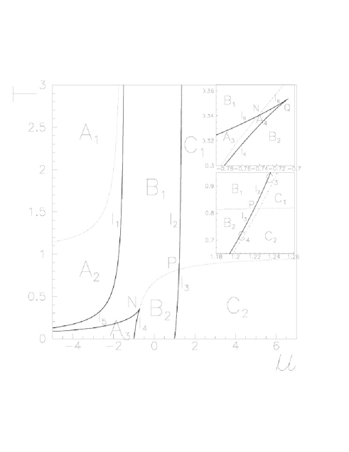
FIG. 8.: The various regions of the plane $\mu-T$ with respect to the roots $a_{k}$ $\left(k=1,2,3\right)$. The characteristics of the roots in the various regions are described in the text. The solid lines ($l_{i}$ $i=1,...,6$) are defind by the vanishing of the discriminant of (A2), namely $\frac{1}{4}\left(-\frac{2}{27}A_{2}+\frac{1}{3}A_{1}A_{2}-A_{0}\right)^{2}+\frac{1}{27}\left(A_{1}-\frac{1}{3}A_{2}^{2}\right)^{3}=0$. The dotted lines are given by Eq. (6) for $\mu<-1.5$ and $\mu\geq-1$. Finally, the dash-dotted line is given by $T=\frac{1-\mu}{\mu-1.5}$ for $1\leq\mu<1.5$. The two insets show an enlargement of the regions around the point $N\simeq\left(-0.74,0.34\right)$ and $P\simeq\left(1.22,0.82\right)$. Notice in particular the existence of the very narrow regions $A_{4},C_{3},C_{4}$.

B Computation of $\Gamma$ and of the density in the case of degenere roots

Here we discuss briefly the computation of the functions $\Gamma\left(t\right)$ and $d\left(t\right)$ when the third degree polynomial $C\left(z\right)$ has no distinct roots (lines $l_{i}$ in Fig. 8). Since the equilibrium solution $z_{s}$ is never degenere, we do not find qualitative differences with respect to the no degenere case; in particular the long time behaviours of $\Gamma$ and $d$ are unchanged.

Firstly we consider the case of one doubly degenere root; let it be for example $a_{2}=a_{3}$ and thus $C\left(z\right)=\left(z-a_{1}\right)\left(z-a_{2}\right)^{2}$. Computing the inverse transform of (31), Eq. (32) has to be replaced by:

$$\Gamma\left(t\right) = \phi_{11}^{P}\left(a_{1}\right)e^{\left(a_{1}/\beta\right)t}-\beta\phi_{11}^{Q}\left(a_{1}\right)\int_{0}^{t}e^{\left(a_{1}/\beta\right)\left(t-u\right)}\frac{I_{1}\left(2u\right)}{u}du$$ (B3)

$$+\phi_{21}^{P}\left(a_{2}\right)\frac{t}{\beta}e^{\left(a_{2}/\beta\right)t}-\beta\phi_{21}^{Q}\left(a_{2}\right)\int_{0}^{t}e^{\left(a_{2}/\beta\right)\left(t-u\right)}\frac{\left(t-u\right)}{\beta}\frac{I_{1}\left(2u\right)}{u}du$$

$$+\phi_{22}^{P}\left(a_{2}\right)e^{\left(a_{2}/\beta\right)t}-\beta\phi_{22}^{Q}\left(a_{2}\right)\int_{0}^{t}e^{\left(a_{2}/\beta\right)\left(t-u\right)}\frac{I_{1}\left(2u\right)}{u}du$$

where $\phi_{11}^{P}\left(a_{1}\right)=\frac{P\left(a_{1}\right)}{C^{\prime}\left(a_{1}\right)}$, $\phi_{11}^{Q}\left(a_{1}\right)=\frac{Q\left(a_{1}\right)}{C^{\prime}\left(a_{1}\right)}$, $\phi_{2l}^{P}\left(a_{2}\right)=\left.\frac{d^{l-1}}{dz^{l-1}}\frac{P\left(z\right)\left(z-a_{2}\right)^{2}}{C\left(z\right)}\right|_{z=a_{2}}$ and $\phi_{2l}^{Q}\left(a_{2}\right)=\left.\frac{d^{l-1}}{dz^{l-1}}\frac{Q\left(z\right)\left(z-a_{2}\right)^{2}}{C\left(z\right)}\right|_{z=a_{2}}$ with $l=1,2\$. Using the integral representation of the modified Bessel function $I_{1}$ we find:

$$\Gamma\left(t\right) = e^{\left(a_{1}/\beta\right)t}S_{1}\left(a_{1}\right)+e^{\left(a_{2}/\beta\right)t}\left[\frac{t}{\beta}S_{2}\left(a_{2}\right)+S_{2}^{\prime}\left(a_{2}\right)\right]$$ (B5)

$$+e^{2t}\left[\beta\phi_{11}^{Q}\left(a_{1}\right)J_{1,a_{1}/2\beta}\left(2t\right)-\frac{1}{2}\phi_{21}^{Q}\left(a_{2}\right)J_{2,a_{2}/2\beta}\left(2t\right)+\beta\phi_{22}^{Q}\left(a_{2}\right)J_{1,a_{2}/2\beta}\left(2t\right)\right]$$

with $S_{1}\left(a_{1}\right)$ given by (40); furthermore

$$S_{2}\left(a_{2}\right) = \phi_{21}^{P}\left(a_{2}\right)-\phi_{21}^{Q}\left(a_{2}\right)\left(\frac{a_{2}-\sqrt{a_{2}^{2}-4\beta^{2}}}{2}\right)$$ (B6)

$$= \left\{\begin{array}[]{ll}\left[\left(a_{2}+2\beta\mu\right)^{2}-\beta^{2}\left(a_{2}+2\beta\mu-1\right)^{2}\right]\frac{1}{a_{2}-a_{1}}&\text{if }a_{2}\text{ satisfies Eq. (\ref{saddle-eq})}\\ \frac{C\left(a_{2}\right)}{a_{2}-a_{1}}=0&\text{else}\end{array}\right.$$ (B9)

and the integrals $J_{k,c}\left(t\right)$ for $k=1,2$ are defined by

$$J_{k,c}\left(t\right)=\frac{1}{\pi}\int_{-1}^{1}\frac{\sqrt{1-x^{2}}}{\left(c-x\right)^{k}}e^{\left(x-1\right)t}dx$$ (B10)

Notice that the integral $J_{1,c}\left(t\right)$ coincides with that defined by Eq. (33); furthermore $J_{2,c}\left(t\right)$ is related to $J_{1,c}\left(t\right)$ by the relation $J_{2,c}\left(t\right)=-\frac{\partial}{\partial c}J_{1,c}\left(t\right).$ If $a_{2}$ does not satisfy Eq. (5), the whole coefficient of $e^{\left(a_{2}/\beta\right)t}$ vanishes since $C\left(a_{2}\right)=C^{\prime}\left(a_{2}\right)=0$. The density is found to be:

$$d\left(t\right) = 1-\frac{T}{2\Gamma\left(t\right)}\left\{\frac{S\left(a_{1}\right)}{a_{1}/2\beta+\mu}\left(e^{\left(a_{1}/\beta\right)t}-e^{-2\mu t}\right)+\frac{S_{2}\left(a_{2}\right)}{a_{2}/2\beta+\mu}\left[\frac{t}{\beta}e^{\left(a_{2}/\beta\right)t}-\frac{e^{\left(a_{2}/\beta\right)t}-e^{-2\mu t}}{2\beta\left(a_{2}/2\beta+\mu\right)}\right]\right.$$ (B14)

$$+\frac{S_{2}^{\prime}\left(a_{2}\right)}{a_{2}/2\beta+\mu}\left(e^{\left(a_{2}/\beta\right)t}-e^{-2\mu t}\right)+\frac{\phi_{11}^{Q}\left(a_{1}\right)\beta}{a_{1}/2\beta+\mu}\left[e^{2t}\left(J_{1,a_{1}/2\beta}\left(2t\right)-J_{1,-\mu}\left(2t\right)\right)-e^{-2\mu t}\left(\widetilde{J}_{1,a_{1}/2\beta}-\widetilde{J}_{1,-\mu}\right)\right]$$

$$-\frac{\phi_{21}^{Q}\left(a_{2}\right)}{2\left(a_{2}/2\beta+\mu\right)}\left[e^{2t}\left(J_{2,a_{2}/2\beta}\left(2t\right)+\frac{J_{1,a_{2}/2\beta}\left(2t\right)-J_{1,-\mu}\left(2t\right)}{a_{2}/2\beta+\mu}\right)+e^{-2\mu t}\left(\widetilde{J}_{2,a_{2}/2\beta}+\frac{\widetilde{J}_{1,a_{2}/2\beta}-\widetilde{J}_{1,-\mu}}{a_{2}/2\beta+\mu}\right)\right]$$

$$\left.+\frac{\phi_{22}^{Q}\left(a_{2}\right)\beta}{a_{2}/2\beta+\mu}\left[e^{2t}\left(J_{1,a_{2}/2\beta}\left(2t\right)-J_{1,-\mu}\left(2t\right)\right)-e^{-2\mu t}\left(\widetilde{J}_{1,a_{2}/2\beta}-\widetilde{J}_{1,-\mu}\right)\right]\right\}$$

where $\widetilde{J}_{k,c}=J_{k,c}\left(0\right)$; one has in particular $\widetilde{J}_{1,c}=c-\sqrt{c^{2}-1}$. We note that the long time behaviour of $J_{k,c}\left(t\right)$ is given by $J_{k,c}\left(t\right)\simeq\frac{1}{\sqrt{2\pi t^{3}}\left(c-1\right)^{k}}$; since it can be shown $\frac{\beta^{2}\phi_{11}^{Q}\left(a_{1}\right)}{a_{1}-2\beta}-\frac{\beta^{2}\phi_{21}^{Q}\left(a_{2}\right)}{\left(a_{2}-2\beta\right)^{2}}+\frac{\beta^{2}\phi_{22}^{Q}\left(a_{2}\right)}{a_{2}-2\beta}=\frac{d}{q_{EA}^{2}}$, one recovers the final results of the Eqs. (44,b), valid in the spin glass phase.

Finally, let us consider the case $a_{1}=a_{2}=a_{3}$ (point Q in Fig. 8): $C\left(z\right)=\left(z-a_{1}\right)^{3}$. One has:

$$\Gamma\left(t\right)=\sum_{l=1}^{3}\left[\frac{\phi_{3l}^{P}\left(a_{1}\right)}{\left(3-l\right)!\left(l-1\right)!}\left(\frac{t}{\beta}\right)^{3-l}+\frac{\beta\phi_{3l}^{Q}\left(a_{1}\right)}{\left(3-l\right)!\left(l-1\right)!}\int_{0}^{t}e^{\left(a_{1}/\beta\right)\left(t-u\right)}\left(\frac{t-u}{\beta}\right)^{3-l}\frac{I_{1}\left(2u\right)}{u}du\right]$$ (B15)

where $\phi_{3l}^{P}\left(a_{1}\right)=\left.\frac{d^{l-1}}{dz^{l-1}}P\left(z\right)\right|_{z=a_{1}}$, $\phi_{3l}^{Q}\left(a_{1}\right)=\left.\frac{d^{l-1}}{dz^{l-1}}Q\left(z\right)\right|_{z=a_{1}}\ l=1,2,3$. Then, using the integral representation of $I_{1}$, one gets:

$$\Gamma\left(t\right) = e^{\left(a_{1}/\beta\right)t}\left[\frac{1}{2}\left(\frac{t}{\beta}\right)^{2}S\left(a_{1}\right)+\left(\frac{t}{\beta}\right)S^{\prime}\left(a_{1}\right)+\frac{1}{2}S^{\prime\prime}\left(a_{1}\right)\right]$$ (B17)

$$+e^{2t}\left[\frac{\phi_{31}^{Q}\left(a_{1}\right)}{4\beta}J_{3,a_{1}/2\beta}\left(2t\right)-\frac{1}{2}\phi_{32}^{Q}\left(a_{1}\right)J_{2,a_{1}/2\beta}\left(2t\right)+\frac{1}{2}\beta\phi_{33}^{Q}\left(a_{2}\right)J_{1,a_{1}/2\beta}\left(2t\right)\right]$$

where

$$S\left(a_{1}\right) = \phi_{31}^{P}\left(a_{1}\right)-\phi_{31}^{Q}\left(a_{1}\right)\left(\frac{a_{1}-\sqrt{a_{1}^{2}-4\beta^{2}}}{2}\right)$$ (B18)

$$= \left\{\begin{array}[]{ll}\left(a_{1}+2\beta\mu\right)^{2}-\beta^{2}\left(a_{1}+2\beta\mu-1\right)^{2}&\text{if }a_{1}\text{ satisfies Eq. (\ref{saddle-eq})}\\ C\left(a_{1}\right)=0&\text{else}\end{array}\right.$$ (B21)

and the integrals $J_{k,c}\left(t\right)$ are defined by (B10) for $k=1,2,3$. In particular one has $J_{3,c}\left(t\right)=\frac{1}{2}\frac{\partial^{2}}{\partial c^{2}}J_{1,c}\left(t\right)$. The coefficient of $e^{\left(a_{1}/\beta\right)t}$ vanishes since $C\left(a_{1}\right)=C^{\prime}\left(a_{1}\right)=C^{\prime\prime}\left(a_{1}\right)=0$. The density is

$$d\left(t\right) = 1-\frac{T}{2\Gamma\left(t\right)}\left\{\frac{\phi_{31}^{Q}\left(a_{1}\right)}{4\beta\left(a_{1}/2\beta+\mu\right)}\left[e^{2t}\left(J_{3,a_{1}/2\beta}\left(2t\right)+\frac{J_{2,a_{1}/2\beta}\left(2t\right)}{a_{1}/2\beta+\mu}+\frac{J_{1,a_{1}/2\beta}\left(2t\right)-J_{1,-\mu}\left(2t\right)}{\left(a_{1}/2\beta+\mu\right)^{2}}\right)\right.\right.$$ (B25)

$$\left.+e^{-2\mu t}\left(\widetilde{J}_{3,a_{1}/2\beta}+\frac{\widetilde{J}_{2,a_{1}/2\beta}}{a_{1}/2\beta+\mu}+\frac{\widetilde{J}_{1,a_{1}/2\beta}-\widetilde{J}_{1,-\mu}}{\left(a_{1}/2\beta+\mu\right)^{2}}\right)\right]$$

$$-\frac{\phi_{32}^{Q}\left(a_{1}\right)}{2\left(a_{1}/2\beta+\mu\right)}\left[e^{2t}\left(J_{2,a_{1}/2\beta}\left(2t\right)+\frac{J_{1,a_{1}/2\beta}\left(2t\right)-J_{1,-\mu}\left(2t\right)}{a_{1}/2\beta+\mu}\right)+e^{-2\mu t}\left(\widetilde{J}_{2,a_{1}/2\beta}+\frac{\widetilde{J}_{1,a_{1}/2\beta}-\widetilde{J}_{1,-\mu}}{a_{1}/2\beta+\mu}\right)\right]$$

$$\left.+\frac{\phi_{33}^{Q}\left(a_{1}\right)\beta}{2\left(a_{1}/2\beta+\mu\right)}\left[e^{2t}\left(J_{1,a_{1}/2\beta}\left(2t\right)-J_{1,-\mu}\left(2t\right)\right)-e^{-2\mu t}\left(\widetilde{J}_{1,a_{1}/2\beta}-\widetilde{J}_{1,-\mu}\right)\right]\right\}$$

where $\widetilde{J}_{k,c}=J_{k,c}\left(0\right)$. From $J_{k,c}\left(t\right)\simeq\frac{1}{\sqrt{2\pi t^{3}}\left(c-1\right)^{k}}$ and $\frac{1}{2}\frac{\beta^{2}\phi_{33}^{Q}\left(a_{1}\right)}{a_{1}-2\beta}-\frac{\beta^{2}\phi_{32}^{Q}\left(a_{1}\right)}{\left(a_{1}-2\beta\right)^{2}}+\frac{\beta^{2}\phi_{31}^{Q}\left(a_{1}\right)}{\left(a_{1}-2\beta\right)^{3}}=\frac{d}{q_{EA}^{2}}$ one gets again the final results of Eqs. (44,b), valid in the spin glass phase.

REFERENCES

- [1] Sompolinsky H. and Zippelius A., Phys. Rev. B 25 (1982) 6860
- [2] Kirkpatrick T.R. and Thiumalai D., Phys. Rev. B 36 (1987) 5388; Phys. Rev. Lett 58 (1987) 2091
- [3] Ciuchi S. and De Pasquale F., Nucl. Phys. B300 (FS22) (1988) 31
- [4] Crisanti A., Horner H. and Sommers H-J., Z. Phys. B 92 (1993) 257
- [5] Cugliandolo L.F. and Kurchan J., Phys. Rev. Lett. 71 (1993) 173
- [6] Cugliandolo L.F. and Kurchan J., J. Phys. A27 (1994) 5749
- [7] Cugliandolo L.F. and Dean D.S., J. Phys. A28 (1995) 4213
- [8] Cugliandolo L.F. and Le Doussal P., Phys. Rev. E53 (1996) 1525
- [9] Bouchaud J.P., Cugliandolo L.F., Kurchan J. and Mezard M., ”Out of equilibrium dynamics in spin glasses and other glassy systems” in ”Spin glasses and random fields” edited by Young A.P. (World Scientific, Singapore, 1997)
- [10] Gotze W., in Liquids, freezing and glass transition, Les Houches (1989), Hansen J.P., Levesque D., Zinn-Justin (North Holland, Amsterdam 1991)
- [11] Bouchaud J.P., Cugliandolo L.F., Kurchan J. and Mezard M., Physica A 226 (1996) 243
- [12] Kosterlitz J.M., Thouless D.J. and Jones R.C., Phys. Rev. Lett. 36 (1976) 1217
- [13] Ghatak S.K.. and Sherrington D., J. Phys. C 10 (1977) 3149; Lage E.J.S and de Almeida J.R.L., J. Phys. C 15 (1982) L1187; Mottishaw P. and Sherrington D., J. Phys. C 18 (1985) 5201; da Costa F.A., Yokoi C.S.O. and Salinas S.R., J. Phys. A 27 (1994) 3365
- [14] Nicodemi M. and Coniglio A., J. Phys. A 30 (1997) L187; Arenzon J., Nicodemi M. and Sellitto M., J. Phys. I France 6 (1996) 1143; Coniglio A., de Candia A., Fierro A. and Nicodemi M., J. Phys. Condens. Matter 11 (1999) A167
- [15] Coniglio A., J. Phys. IV France 3 (1993) C1-1; Il Nuovo Cimento D 16 (1994) 1027; Physica A 266 (1999) 379; Physica A (2000) 129
- [16] Nicodemi M., Coniglio A. and Herrmann H.J., Phys. Rev. E 55 (1997) 3962; Coniglio A. and Nicodemi M., Phys. Rev. Lett. 82 (1999) 916; Nicodemi M., Phys. Rev. Lett. 82 (1999) 3734; Coniglio A. and Nicodemi M., J. Phys. Condens. Matter 12 (2000) 6601
- [17] Sellitto M., Nicodemi M. and Arenzon J., J. Phys. I France 7 (1997) 945; Schreiber G.R., Eur. Phys. J B9 (1999) 479
- [18] Crisanti A. and Leuzzi L., cond-mat 0204349
- [19] Lippiello E. and Zannetti M., Phys. Rev. E 61 (2000) 3369
- [20] Caiazzo A., Coniglio A. and Nicodemi M., in preparation
- [21] As static properties are concerned, the two Ising lattice fields can be replaced by the single spin-1 field apart from a simple rescaling of . The change of variables in Eq. (3) is rewritten in terms of as .
- [22] Traditionally, schematic MCT deals with a one time correlator which, in our framework, is to be identified by at equilibrium, normalized by its equal time value: .