]http://www.mech.kochi-tech.ac.jp/cheon/

Evolutionary Stability of Ecological Hierarchy

Taksu Cheon taksu.cheon@kochi-tech.ac.jp [ Laboratory of Physics, Kochi University of Technology, Tosa Yamada, Kochi 782-8502, Japan
(January 31, 2003)
Abstract

A self-similar hierarchical solution that is both dynamically and evolutionarily stable is found to the multi dimensional Lotka-Volterra equation with a single chain of prey-predator relations. This gives a simple and natural explanation to the key features of hierarchical ecosystems, such as its ubiquity, pyramidal population distribution, and higher aggressiveness among higher trophic levels.

Lotka-Volterra equation, Trophic pyramid, Self-similarity
pacs:
87.23.Kg, 89.75.Da, 05.45.-a
preprint:

From bacterial colony to human society, hierarchical structure is one of the most universal features of ecological systems. It is typically realized as a trophic pyramid with exponentially larger populations for lower trophic levels. The ubiquity of this hierarchy in nature suggests the existence of a simple and robust mechanism behind it.

Let us consider an ecosystem of $N$ species whose populations $x_{1}(t)$, $x_{2}(t)$, $...$, $x_{N}(t)$ are described by a set of coupled differential equations with parameters that represent the environmental conditions MA72 ; HS88 . Then, the robustness of ecological structures is expressed as the presence and stability of fixed point solutions. The stability should be considered on two levels of different time-scales. The short-term dynamical stability is the stability against the perturbation in the dynamical variables $x_{n}$, while the long-term stability is related to the robustness of the solutions against the secular variation of environmental parameters. When some environmental parameters are at the disposal of a certain species, natural selection will lead to the realization of the parameter value that maximizes the population of that species. This is the concept of evolutionary stability MS82 ; AX97 .

There are several numerical simulations of multi-species ecosystems that show the spontaneous emergence of multi-trophic structure LA01 ; QH02 . The models employ coupled differential equations with stochastic parameter variation subjected to evolutionary selection rules. These results indicate that pyramidal hierarchy is an evolutionarily stable configuration of ecosystems irrespective to the fine detail of the model. It is high time to search for a simple and clear theoretical explanation before further numerical calculations with increasingly “realistic” settings are to be pursued.

In this article, we consider ecosystems modeled by the Lotka-Volterra equation describing $N$ species that form a single vertical chain of prey-predator relations. We intend to prove the existence of hierarchical solutions that are stable both dynamically and evolutionarily.

Let us begin with the two species prey-predator Lotka-Volterra equation

$\displaystyle\dot{x_{1}}$ $\displaystyle=$ $\displaystyle bx_{1}-ax_{1}^{2}-\rho_{2}x_{1}x_{2}$ (1)
$\displaystyle\dot{x_{2}}$ $\displaystyle=$ $\displaystyle-d_{2}x_{2}+f_{2}\rho_{2}x_{1}x_{2}.$

Here $b$ is the reproduction rate of the prey $x_{1}$ and $a$ the environmental limitation factor to its growth. The parameter $d_{2}$ is the decay rate of the predator $x_{2}$ which will not subsist without preying on $x_{1}$ with the rate of aggression $\rho_{2}$. The factor $f_{2}$ represents the combination of the efficiency of the predation and the average mass ratio between prey and predator individuals. All parameters are positive real numbers. Although the dynamical variables $x_{n}$ are treated as continuous quantities here, they are approximations of the actual integer populations. Moreover, in real life, there is a threshold number for a population under which a species is not viable. As is immediately identified, (1) has a nontrivial fixed point solution $x_{1}(t)=X_{1}$, $x_{2}(t)=X_{2}$ where $X_{1}$ and $X_{2}$ satisfy

$\displaystyle b-aX_{1}-\rho_{2}X_{2}$ $\displaystyle=$ $\displaystyle 0,$ (2)
$\displaystyle-d_{2}+f_{2}\rho_{2}X_{1}$ $\displaystyle=$ $\displaystyle 0.$

The eigenvalues $\lambda$ of the linearized map around the fixed point are given by

$\displaystyle\lambda=-{{1}\over{2q}}\left(1\pm\sqrt{1-4d_{2}q(bq-1)}\right),\quad q\equiv{f_{2}\rho_{2}\over{ad_{2}}}.$ (3)

Therefore, the fixed point is dynamically stable when we have $f_{2}\rho_{2}b$ $>ad_{2}$. Since, in this work, we are primarily concerned with the “populous” regime, $b\gg a$, this condition is almost always satisfied.

Let us now assume that the aggression parameter $\rho_{2}$ is a quantity that is at the disposal of the predator $x_{2}$ through a long term “behavioral change”. That is, we regard $X_{1}$ and $X_{2}$ as functions of $\rho_{2}$. Naturally, a change in $\rho_{2}$ would be directed toward the maximization of the predator population $x_{2}$ through evolutionary selection. We further assume that the time scale for the change of $\rho_{2}$ is substantially larger than the time scale for the variation of $x_{1}(t)$ and $x_{2}(t)$. Then, irrespective to the precise mechanism of the variation of $\rho_{2}$, one eventually ends up with the value $\rho_{2}^{\star}$ that maximizes $X_{2}(\rho_{2})$. With the notation $X_{i}^{\star}$ $\equiv X_{i}(\rho_{2}^{\star})$, we have

$\displaystyle\rho_{2}^{\star}={{2ad_{2}}\over{f_{2}b}},\quad X_{2}^{\star}={{f_{2}b^{2}}\over{4ad_{2}}},\quad X_{1}^{\star}={b\over{2a}},$ (4)

which represents the evolutionarily stable solution. The solution is always dynamically stable, since, at these values, the real part of the eigenvalue of linearized map (3) never becomes positive. The stability against parametric variation of $\rho_{2}$ can be judged by

$\displaystyle{{d^{2}X_{2}^{\star}}\over{d\rho_{2}^{2}}}=-{b\over{{\rho_{2}^{\star}}^{3}}}.$ (5)

Our result shows that the optimal aggression rate from the stand point of the predator is to hunt the prey down to one half of its natural stability point $b/a$ that is reached by $x_{1}$ when left alone. Already at this point, (4) gives us some insights. When $b$ and $d_{2}$ are comparable quantities, the predator population $X_{2}^{\star}$ is suppressed by the factor $f_{2}/2$ compared to the prey $X_{1}^{\star}$. Since $f_{2}$ is typically smaller than 1, we tend to have a small number of predators supported by a large pool of prey biomass as a stable configuration. Another interesting point is that the milder environment signified by a higher value of $b/a$ will increase both $X_{1}^{\star}$ and $X_{2}^{\star}$ while reducing the optimal aggression rate $\rho_{2}^{\star}$ of the predator. This principle of noblesse oblige is a widely observed, but nonetheless nontrivial aspect of life. This is corroborated, for example, by recent field work observation on slave-making ants FH01 .

According to (4), the only way for the prey $x_{1}$ to increase its equilibrium population is to “improve the environment” by increasing $b/a$, when there is any such mean available to it. An intriguing fact is that “improving defensive shield” by decreasing $f_{2}$ will not benefit $x_{1}$ directly; it simply decreases the predator population $X_{2}^{\star}$. However, when $X_{2}$ is close to the viability threshold, a decreasing $f_{2}$ would be a sensible strategy for $x_{1}$, since that could drive $x_{2}$ out of existence, which would result in the instant doubling of $X_{1}^{\star}$.

Next, we consider the case of $N=3$ species that forms a single chain of prey-predator relations CP02 :

$\displaystyle\dot{x_{1}}$ $\displaystyle=$ $\displaystyle bx_{1}-ax_{1}^{2}-\rho_{2}x_{1}x_{2},$ (6)
$\displaystyle\dot{x_{2}}$ $\displaystyle=$ $\displaystyle-d_{2}x_{2}+f_{2}\rho_{2}x_{1}x_{2}-\rho_{3}x_{2}x_{3},$
$\displaystyle\dot{x_{3}}$ $\displaystyle=$ $\displaystyle-d_{3}x_{3}+f_{3}\rho_{3}x_{2}x_{3}.$

The fixed point solution is obtained as

$\displaystyle b-aX_{1}-\rho_{2}X_{2}$ $\displaystyle=$ $\displaystyle 0,$ (7)
$\displaystyle-d_{2}+f_{2}\rho_{2}X_{1}-\rho_{3}X_{3}$ $\displaystyle=$ $\displaystyle 0,$
$\displaystyle-d_{3}+f_{3}\rho_{3}X_{2}$ $\displaystyle=$ $\displaystyle 0.$

By rearranging the first two equations, we obtain

$\displaystyle b_{2}-a_{2}X_{2}-\rho_{3}X_{3}$ $\displaystyle=$ $\displaystyle 0,$ (8)
$\displaystyle-d_{3}+f_{3}\rho_{3}X_{2}$ $\displaystyle=$ $\displaystyle 0.$

with

$\displaystyle a_{2}\equiv{{f_{2}\rho_{2}^{2}}\over a},\quad b_{2}\equiv{{f_{2}b\rho_{2}}\over{a}}-d_{2}.$ (9)

The problem is therefore reduced to the $N=2$ case with the predator $x_{3}$ and effectively self-sustaining prey $x_{2}$ which has reproduction and limiting coefficients $b_{2}$ and $a_{2}$. If the top predator, driven by evolutionary selection, tries to maximize its equilibrium population $X_{3}$ by varying $\rho_{3}$, it will reach the optimum given by

$\displaystyle\rho_{3}^{(\star)}={{2a_{2}d_{3}}\over{f_{3}b_{2}}},\quad X_{3}^{(\star)}={{f_{3}b_{2}^{2}}\over{4a_{2}d_{3}}},\quad X_{2}^{(\star)}={{b_{2}}\over{2a_{2}}}.$ (10)

The fact that these values are optimum only with a given $\rho_{2}$ is indicated by the bracketed asterisk. From the relation $\rho_{3}^{(\star)}X_{3}^{(\star)}$ $=b_{2}/2$, one can rewrite the first two equations of (7) as

$\displaystyle{b\over 2}-a\left({X_{1}-{b\over{2a}}}\right)-\rho_{2}X_{2}$ $\displaystyle=$ $\displaystyle 0$ (11)
$\displaystyle-{d_{2}\over 2}+f_{2}\rho_{2}\left({X_{1}-{b\over{2a}}}\right)$ $\displaystyle=$ $\displaystyle 0.$

This is essentially the same relationship as in the $N=2$ case (2), with an extra factor $1/2$ in front of the first terms, and the shift in $X_{1}$ in the socond. We should now suppose that the middle predator $x_{2}$ will, in a long run, adjust its aggression rate $\rho_{2}$ toward the prey $x_{1}$ and maximize $X_{2}$. We then obtain the solution

$\displaystyle\rho_{2}^{\star}={{2ad_{2}}\over{f_{2}b}},\quad X_{2}^{\star}={{f_{2}b^{2}}\over{8ad_{2}}},\quad X_{1}^{\star}={{3b}\over{4a}},$ (12)

which in turn yields

$\displaystyle\rho_{3}^{\star}={{8ad_{2}d_{3}}\over{f_{2}f_{3}b^{2}}},\quad X_{3}^{\star}={f_{2}f_{3}b^{2}\over{16ad_{3}}}.$ (13)

Note the fact that $\rho_{2}^{\star}$ here is identical to the $N=2$ case. We also obtain parametric stability measures as

$\displaystyle{{d^{2}X_{2}^{\star}}\over{d\rho_{2}^{2}}}=-{b\over{2{\rho_{2}^{\star}}^{3}}},\quad{{d^{2}X_{3}^{\star}}\over{d\rho_{2}^{2}}}=-{{d_{2}}\over{{\rho_{3}^{\star}}^{3}}},$ (14)

which indeed prove the evolutionary stability of the solution.
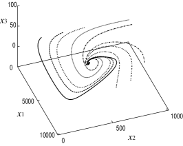
Refer to caption
Figure 1: The phase space profile of a $N=3$ system at evolutionarily stable parameter value. The parameters are set to be $b=1$, $a=1/10000$, $d_{2}=1/3$, $d_{3}=1/5$, $f_{2}=1/10$, $f_{3}=1/5$. The optimal aggression rates are calculated as $\rho_{2}^{\star}=1/1500$ and $\rho_{3}^{\star}=1/375$. All orbits approach the fixed point $(X_{1}^{\star},X_{2}^{\star},X_{3}^{\star})$ $=(7500,375,64.5)$.

In Fig.1, the phase space profile of one such example of evolutionarily stable $N=3$ system is depicted. With consideration at each stage (8) and (11), it is easy to see that this evolutionarily stable solution is also dynamically stable for all parameter values. In effect, the single-chain $N=3$ Lotka-Volterra equation is broken into two $N=2$ equations with essentially the same structure, albeit with an additional factor for the lower chain.

When $d_{2}$ and $d_{3}$ are comparable quantities, the population of the top trophic level $X_{3}^{\star}$ is inherently suppressed by the factor $f_{3}/2$ compared to that of $X_{2}^{\star}$, giving a pyramidal profile to the trophic structure. It is amusing to note that, from the stand point of the lowest trophic species, an $N=3$ system, in which two thirds of its natural population is left alive, is considerably more “benign” than an $N=2$ system.

The preceding proof for the $N=3$ solution suggests its generalization to arbitrary $N$. This is achieved through the realization that the fixed point equation for any mid-level population $x_{n}$ can have both purely prey-like and purely predator-like representations. Let us start with the $N$ vertically-coupled Lotka-Volterra equation with evolutionarily adjustable aggression parameter $\rho_{n}$ for each species $x_{n}$

$\displaystyle\dot{x}_{1}$ $\displaystyle=$ $\displaystyle bx_{1}-ax_{1}^{2}-\rho_{2}x_{1}x_{2},$ (15)
$\displaystyle\dot{x}_{2}$ $\displaystyle=$ $\displaystyle-d_{2}x_{2}+f_{2}\rho_{2}x_{1}x_{2}-\rho_{3}x_{2}x_{3},$
$\displaystyle\vdots$
$\displaystyle\dot{x}_{n}$ $\displaystyle=$ $\displaystyle-d_{n}x_{n}+f_{n}\rho_{n}x_{n-1}x_{n}-\rho_{n+1}x_{n}x_{n+1},$
$\displaystyle\vdots$
$\displaystyle\dot{x}_{N}$ $\displaystyle=$ $\displaystyle-d_{N}x_{N}+f_{N}\rho_{N}x_{N-1}x_{N}.$

In general, a trophic level can comprise several competing species. In our simplified treatment, however, such species are lumped into a single population variable. The equations for the nontrivial fixed point $(X_{1},...,X_{N})$ are

$\displaystyle b-aX_{1}-\rho_{2}X_{2}$ $\displaystyle=$ $\displaystyle 0,$ (16)
$\displaystyle-d_{2}+f_{2}\rho_{2}X_{1}-\rho_{3}X_{3}$ $\displaystyle=$ $\displaystyle 0,$
$\displaystyle\vdots$
$\displaystyle-d_{n}+f_{n}\rho_{n}X_{n-1}-\rho_{n+1}X_{n+1}$ $\displaystyle=$ $\displaystyle 0,$
$\displaystyle\vdots$
$\displaystyle-d_{N}+f_{N}\rho_{N}X_{N-1}$ $\displaystyle=$ $\displaystyle 0.$

Apart from the species with the highest trophic level $x_{N}$, each of these can be transformed to the form

$\displaystyle b_{n}-a_{n}X_{n}-\rho_{n+1}X_{n+1}$ $\displaystyle=$ $\displaystyle 0,$ (17)

with the recursive definition

$\displaystyle a_{n}=f_{n}\rho_{n}^{2}{1\over{a_{n-1}}},\quad b_{n}=f_{n}\rho_{n}{{b_{n-1}}\over{a_{n-1}}}-d_{n}.$ (18)

Rewriting (17), we obtain the “slave” form

$\displaystyle\eta_{n}b_{n}-a_{n}\left(X_{n}-(1-\eta_{n}){b_{n}\over a_{n}}\right)-\rho_{n+1}X_{n+1}=0$ (19)

for $n=1,..,N-1$. Let us now assume the relation

$\displaystyle\rho_{n+1}^{(\star)}X_{n+1}^{(\star)}$ $\displaystyle=$ $\displaystyle{{\eta_{n}b_{n}}\over 2}.$ (20)

If we combine (16), (20) with a requirement

$\displaystyle 1-\eta_{n}={{\eta_{n+1}}\over 2},$ (21)

we obtain the “master” form

$\displaystyle-\eta_{n}d_{n+1}+f_{n+1}\rho_{n+1}\left(X_{n}-(1-\eta_{n}){b_{n}\over a_{n}}\right)=0$ (22)

for $n=1,..,N-1$. The equations (16) are now decoupled to $(N-1)$ pairs of prey-predator equations (19) and (22). We then have

$\displaystyle\rho_{n+1}^{(\star)}={2a_{n}d_{n+1}\over{f_{n+1}b_{n}}},$ (23)

and

$\displaystyle X_{n+1}^{(\star)}=\eta_{n}{{f_{n+1}b_{n}^{2}}\over{4a_{n}d_{n+1}}},\quad X_{n}^{(\star)}=(2-\eta_{n}){{b_{n}}\over{2a_{n}}}.$ (24)

This result justifies the assumption (20) a posteriori, and the whole procedure becomes consistent. From the last equation of (16), we observe that $\eta_{N-1}$ should be set to one, which results in $\eta_{N-2}=1/2$, $\eta_{N-3}=3/4$, $\cdots$. We finally obtain the following explicit forms for the evolutionarily and dynamically stable solution:

$\displaystyle X_{1}^{\star}$ $\displaystyle=$ $\displaystyle{B_{N}b\over{2^{N-1}a}},$ (25)
$\displaystyle X_{2}^{\star}$ $\displaystyle=$ $\displaystyle{B_{N-1}f_{2}b^{2}\over{2^{N}ad_{2}}},\quad\rho_{2}^{\star}={{2ad_{2}}\over{f_{2}b}},$
$\displaystyle\vdots$
$\displaystyle X_{N}^{\star}$ $\displaystyle=$ $\displaystyle{B_{1}f_{2}\cdots f_{N}b^{2}\over{2^{2N-2}ad_{3}}},\quad\rho_{N}^{\star}={{2^{2N-3}ad_{2}d_{3}}\over{f_{2}\cdots f_{N}b^{2}}}.$

The stability with respect to the variation $\rho_{n}$ is given by

$\displaystyle{{d^{2}X_{2}^{\star}}\over{d\rho_{2}^{2}}}=-{B_{N-1}b\over{2^{N-2}{\rho_{2}^{\star}}^{3}}},\quad{{d^{2}X_{3}^{\star}}\over{d\rho_{3}^{2}}}=-{B_{N-2}b\over{2^{N-3}{\rho_{3}^{\star}}^{3}}},$ (26)
$\displaystyle\cdots\quad{{d^{2}X_{N}^{\star}}\over{d\rho_{N}^{2}}}=-{B_{1}b\over{{\rho_{N}^{\star}}^{3}}}.$

Here the coefficient $B_{n}$ is a variant of the Fibonacci series defined by

$\displaystyle B_{n+2}=B_{n+1}+2B_{n},\quad B_{1}=B_{2}=1.$ (27)

Some of the numbers are $B_{3}=3$, $B_{4}=5$, $B_{5}=11$, $B_{6}=21$, $B_{7}=43$, $\cdots$.

Table 1: The evolutionarily stable hierarchical population for $N$ species Lotka-Volterra equation up to $N=5$. $X_{n}^{\star}$ is the population of $n$-th trophic level, and $\rho_{n}^{\star}$ its aggression rate toward its prey.
$N=1$
$n$ $X_{n}^{\star}$ $\rho_{n}^{\star}$
1 ${b\over{a}}$
$N=2$
$n$ $X_{n}^{\star}$ $\rho_{n}^{\star}$
2 ${f_{2}b^{2}\over{4ad_{2}}}$ ${{2ad_{2}}\over{f_{2}b}}$
1 ${b\over{2a}}$
$N=3$
$n$ $X_{n}^{\star}$ $\rho_{n}^{\star}$
3 ${f_{2}f_{3}b^{2}\over{16ad_{3}}}$ ${{8ad_{2}d_{3}}\over{f_{2}f_{3}b^{2}}}$
2 ${f_{2}b^{2}\over{8ad_{2}}}$ ${{2ad_{2}}\over{f_{2}b}}$
1 ${3b\over{4a}}$
$N=4$
$n$ $X_{n}^{\star}$ $\rho_{n}^{\star}$
4 ${f_{2}f_{3}f_{4}b^{2}\over{64ad_{4}}}$ ${{32ad_{3}d_{4}}\over{f_{2}f_{3}f_{4}b^{2}}}$
3 ${f_{2}f_{3}b^{2}\over{32ad_{3}}}$ ${{8ad_{2}d_{3}}\over{f_{2}f_{3}b^{2}}}$
2 ${3f_{2}b^{2}\over{16ad_{2}}}$ ${{2ad_{2}}\over{f_{2}b}}$
1 ${5b\over{8a}}$
$N=5$
$n$ $X_{n}^{\star}$ $\rho_{n}^{\star}$
5 ${f_{2}f_{3}f_{4}f_{5}b^{2}\over{256ad_{5}}}$ ${{128ad_{4}d_{5}}\over{f_{2}f_{3}f_{4}f_{5}b^{2}}}$
4 ${f_{2}f_{3}f_{4}b^{2}\over{128ad_{4}}}$ ${{32ad_{3}d_{4}}\over{f_{2}f_{3}f_{4}b^{2}}}$
3 ${3f_{2}f_{3}b^{2}\over{64ad_{3}}}$ ${{8ad_{2}d_{3}}\over{f_{2}f_{3}b^{2}}}$
2 ${5f_{2}b^{2}\over{32ad_{2}}}$ ${{2ad_{2}}\over{f_{2}b}}$
1 ${11b\over{16a}}$

In table I, the hierarchical solutions up to $N=5$ are listed. The most notable feature is of course the exponentially smaller population in higher trophic levels. Assuming $d_{n}\approx b$ for all $n$, we have a decrease in the population by factor $f_{n}/2$ for each increase of one trophic level. Since $f_{n}$ is in general substantially smaller than one, we get a pyramidal hierarchy with a steep exponential decrease. We should also mention the self-similarity of the solution: For any given trophic level, the portion of its “natural” population saved from exploitation by higher trophic levels varies like $1/2$, $3/4$, $5/8$, $\cdots$, whenever more trophic levels are added on top. On the other hand, its optimal aggression rate is unaffected by the presence of higher trophic levels. A higher value of $\rho_{n}^{\star}$ for larger $n$ is a direct result of the scarcity of its prey.

Ultimately, the quantity $b/a$ gives the base biomass, on top of which the whole trophic pyramid structure is built. Since there is a minimum population for the highest trophic species to be viable, this naturally puts a limit to the maximum number for the trophic hierarchy of an ecosystem with a given base biomass.

In summary, within the framework of a single vertical food chain model, a pyramidal self-similar hierarchy is found in Lotka-Volterra system. It might be possible to generalize our results to models with plural species in each trophic levels. Hopefully, the search for generic properties of Lotka-Volterra system along this line shall provide a solid backbone for experimental and numerical studies of ecosystems.

The author wishes to thank Izumi Tsutsui, Takuma Yamada, Koji Sekiguchi and David Greene for helpful discussions and useful comments.

References

  • (1) R.M. May, Nature, 261, 459-467 (1976).
  • (2) J. Hofbauer and K. Sigmund: The Theory of Evolution and Dynamical Systems, (Cambridge Univ. Press, 1988).
  • (3) J. Maynard Smith, Evolution and the theory of games, (Cambridge Univ. Press, Cambridge, 1982).
  • (4) R. Axelrod, The Complexity of Cooperation: Agent-Based Models of Competition and Cooperation (Princeton Univ. Press, 1997).
  • (5) M. Lassig, U. Bastolla, S.C. Manrubia and A. Valleriani, Phys. Rev. Lett. 86, 4418-4421 (2001).
  • (6) C. Quince, P.G. Higgs and A.J. McKane, arXiv.org, nlin.AO/0105057 (2001).
  • (7) S. Foitzik, C.J. DeHeer, D.N. Hunjan and J.M. Herbers, Proc. Roy. Soc. London B268, 1139-1146 (2001) .
  • (8) E. Chauvet, J. Paullet, J.P. Previte and Z. Walls, Math. Magazine 75, 243-255 (2002).