Interaction among particles with fractionalized quantum numbers in one dimensional samples

Abstract

The elementary excitations of strongly correlated one-dimensional electronic systems - spinons and holons - are discussed in an exact solution of the Haldane-Shastry and Kuramoto-Yokoyama model. We derive and exactly solve the equation of motion both for the two-spinon wavefunction and for the one-spinon, one-holon wavefunction. By solving the equations of motion we find the spinon-spinon and spinon-holon interaction to be a short-range attraction. The physical consequences of such an attraction on the spin-form factor and on the hole-spectral function are also worked out.

]

I Introduction

Phenomenological Landau’s Fermi liquid theory [1] describes many of the condensed matter systems. The basic assumption of Landau’s theory is that the spectrum of the interacting Fermi liquid may be adiabatically deformed to the spectrum of a noninteracting Fermi gas. Equivalently, one may say that the interaction strength can be continuously increased from 0 (Fermi gas) to its Fermi Liquid value without hitting a singular point. The excitations of a Fermi liquid can be continuously deformed to electrons and holes and are referred to as quasiparticles and quasiholes, respectively.

In a “non-Fermi liquid” such a scenario does not apply. Typical examples of non-Fermi liquids are the one-dimensional strongly correlated electronic systems. The elementary excitations of these systems are collective modes carrying charge 1, but no spin (“holons”), and modes carrying spin-1/2, but no charge (“spinons”). Originally found as elementary excitations of spin-1/2 one-dimensional antiferromagnetic spin chains [2, 3], spinons appear as localized spin-1/2 spin defects, embedded in an otherwise featureless spin-singlet spin-liquid state. Spinons and holons carry “fractions” of the quantum numbers of spin waves and/or holes.

In these lectures we analyze the dynamics of spinons and holons in one-dimensional electron-systems close to half filling. In particular, we study their interaction in the framework of simple, exactly solvable model, using a formalism different from the usual Bethe-ansatz approach [4]. Such an approach treats collective modes of strongly correlated systems (spinons, holons, etc.) as quantum mechanical particles. In particular, it is possible to associate a two-body wavefunction to a two-spinon or to a spinon-holon pair. The corresponding equation of motion can be straightforwardly solved. The form of the interaction potential in the “Schrödinger” operator and the behavior of the solution as a function of the separation among the particles indicates a short-range attraction.

In the thermodynamic limit, the spinon-spinon and spinon-holon attraction drives the low-energy physics of one-dimensional antiferromagnets and strongly-correlated insulators. It is responsible for the sharp features at threshold in the spin structure factor, and in the hole spectral function. These features have been experimentally observed [5, 6] and they provide an important evidence for a short-range attractive force.

The notes are organized as follows:

• In Section II we introduce the Haldane-Shastry model of a one-dimensional antiferromagnet. We study in some details its basic features, its ground state and its elementary excitations;

• In Section III we discuss the two-spinon wavefunction, together with the corresponding equation of motion, its solution, and physical interpretation. We prove the existence of a short-range attraction among spinons;

• In Section IV we consider one-holon and one-spinon states, within the framework of the Kuramoto-Yokoyama model which is the supersymmetric extension of the Haldane-Shastry model;

• In Section V we study the one-spinon one-holon wavefunction. We solve the corresponding equation of motion, and study in detail the basic features of the solution. Finally, we prove the existence of a short-range spinon-holon attraction;

• In Section VI we spell out the physical consequences of the attraction between spinons and holons. We trderive its effects on the dynamical spin structure factor in one dimensional antiferromagnets and on the angle-resolved hole spectral function in one-dimensional insulators;

• In Section VII we provide our conclusions.

II The Haldane-Shastry model of a one-dimensional antiferromagnet and its elementary excitations

Spinons appear as elementary excitations of one-dimensional half-odd spin antiferromagnets. We explore the dynamics of spinons in the framework of the Haldane-Shastry (HS) model of a spin-1/2 antiferromagnetic chain [7, 8].

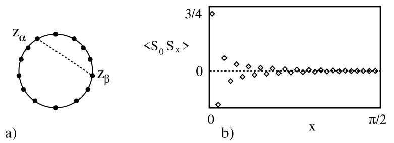
FIG. 1.: a) Haldane-Shastry interaction; b) Spin-spin static correlations in the ground state of the Haldane-Shastry model.

The HS model is a system of spin 1/2 particles lying at the sites of a lattice with periodic boundary conditions. The lattice may be thought of as “wrapped” around a circle. The interaction among the spins is antiferromagnetic, with interaction strength $J$, and inversely proportional to the square of the chord between the corresponding sites. Let $N$ be the number of lattice sites, so that a generic point on the lattice will be labeled by $\alpha=1,\ldots,N$. Let us also define the analytic coordinate on the lattice, $z_{\alpha}=\exp\biggl{[}2\pi i\alpha/N\biggr{]}$. The HS-model Hamiltonian reads:

$${\cal H}_{HS}=\frac{J}{2}\left(\frac{2\pi}{N}\right)^{2}\sum_{\alpha\neq\beta=1}^{N}\frac{{\bf S}_{\alpha}\cdot{\bf S}_{\beta}}{|z_{\alpha}-z_{\beta}|^{2}}$$ (1)

where ${\bf S}_{\alpha}$ is the spin at site $\alpha$ ($({\bf S}_{\alpha})^{2}=3/4)$.

Due to the magic of analytic variables on the circle, $z_{\alpha}^{*}=1/z_{\alpha}$, the interaction in Eq.(1) is, in fact, an analytic function of the $z_{\alpha}$’s. This allows us to work out the action of ${\cal H}_{HS}$ on many-body states, depending on the $z_{\alpha}$’s, in terms of differential operators acting on the analytic extension of the corresponding wavefunctions.

${\cal H}_{\rm HS}$ clearly has the global $SU(2)$-symmetry generated by the total spin ${\bf S}=\sum_{\alpha=1}^{N}{\bf S}_{\alpha}$. It also posses an additional symmetry, corresponding to total spin-current conservation and generated by the operator ${\bf\Lambda}$, given by:

$${\bf\Lambda}=\frac{i}{2}\sum_{\alpha<\beta=1}^{N}\biggl{(}\frac{z_{\alpha}+z_{\beta}}{z_{\alpha}-z_{\beta}}\biggr{)}({\bf S}_{\alpha}\times{\bf S}_{\beta})$$ (2)

that is, one has:

$\displaystyle[{\cal H}_{\rm HS},{\bf S}]=[{\cal H}_{\rm HS},{\bf\Lambda}]=0$

The action of ${\cal H}_{\rm HS}$ on the ground state and on one- and two-spinon collective states of the system will be the subject of the remaining part of this Section.

A Ground state of ${\cal H}_{\rm HS}$

Let $|\Psi_{\rm GS}\rangle$ be the ground state of ${\cal H}_{\rm HS}$. Due to the low-dimensionality, in 1D quantum antiferromagnets with short-range correlations, we cannot expect $|\Psi_{\rm GS}\rangle$ to order. Rather than being realized as a one-dimensional antiferromagnetic state with Neél order, the ground state of the system is given by a one-dimensional spin-liquid state, with spin density uniform over length scales of the order of the lattice step. The ground state also has short-range correlations and no net magnetization. For the HS model, in the even-$N$-case, $|\Psi_{\rm GS}\rangle$ is expressed in terms of its components on states of the Fock space with $N/2$ spin-$\uparrow$, the remaining ones being $\downarrow$. In particular, let $|z_{1},\ldots,z_{N/2}\rangle$ be defined as:

$$|z_{1},\ldots,z_{\frac{N}{2}}\rangle=\prod_{j=1}^{\frac{N}{2}}S_{j}^{+}|\downarrow,\ldots,\downarrow\rangle$$ (3)

where $|\downarrow,\ldots,\downarrow\rangle$ is the fully polarized states with all the spins at the lattice sites being $\downarrow$, while $z_{1},\ldots,z_{N/2}$ are $N/2$-lattice coordinates. We define $|\Psi_{\rm GS}\rangle$ by:

$$\langle z_{1},\ldots,z_{\frac{N}{2}}|\Psi_{\rm GS}\rangle=\Psi_{\rm GS}(z_{1},\ldots,z_{\frac{N}{2}})=\prod_{i<j=1}^{\frac{N}{2}}(z_{i}-z_{j})^{2}\prod_{t=1}^{\frac{N}{2}}z_{t}$$ (4)

${\cal H}_{\rm HS}$ can be traded for a differential operator, when acting on functions of the $z_{\alpha}$’s as discussed in detail, for instance, in [9]. Here we outline the main idea and briefly sketch the basic steps of the derivation.

First of all, we have to split the scalar product ${\bf S}_{\alpha}\cdot{\bf S}_{\beta}$ into $(S_{\alpha}^{+}S_{\beta}^{-}+S_{\alpha}^{-}S_{\beta}^{+})/2+S_{\alpha}^{z}S_{\beta}^{z}$ and to separately consider the action of the various operators on the ground state. Therefore, let us observe that $[S_{\alpha}^{+}S_{\beta}^{-}\Psi_{GS}](z_{1},\ldots,z_{M})$ is different from zero only if one of the arguments $z_{1},\ldots,z_{N/2}$ equals $z_{\alpha}$. By Taylor expanding the corresponding function, we obtain:

$$[\biggl{\{}\sum_{\beta\neq\alpha}^{N}\frac{S_{\alpha}^{+}S_{\beta}^{-}}{\mid\!z_{\alpha}-z_{\beta}\!\mid^{2}}\biggr{\}}\Psi_{GS}](z_{1},\ldots,z_{M})=\sum_{\ell=0}^{N-2}\sum_{j=1}^{M}\frac{z_{j}^{\ell+1}}{\ell!}A_{l}(\frac{\partial^{\ell}}{\partial z_{j}^{\ell}})\biggl{\{}\frac{\Psi_{GS}(\{z_{j}\})}{z_{j}}\biggr{\}}\;\;\;.$$ (5)

(where $\{z_{j}\}$ is a shorthand for $\{z_{1},\ldots,z_{M}\}$).

The coefficients $A_{l}$ are calculated in [9, 10]. In particular, it is possible to show that they are all zero for $N>l>2$. Therefore, we can rewrite Eq.(5) as:

$$\sum_{j=1}^{M}\biggl{\{}\frac{(N-1)(N-5)}{12}z_{j}-\frac{N-3}{2}z_{j}^{2}\frac{\partial}{\partial z_{j}}+\frac{1}{2}z_{j}^{3}\frac{\partial^{2}}{\partial z_{j}^{2}}\biggr{\}}\biggl{\{}\frac{\Psi_{GS}(z_{1},\ldots,z_{M})}{z_{j}}\biggr{\}}$$

$$=\biggl{\{}-\frac{N}{8}-\sum_{j\neq k}^{M}\frac{1}{\mid\!z_{j}-z_{k}\!\mid^{2}}\biggr{\}}\Psi_{GS}(z_{1},\ldots,z_{M})\;\;\;.$$ (6)

where, in deriving Eq.(6), we have used the identity:

$$\frac{z_{\alpha}^{2}}{(z_{\alpha}-z_{\beta})(z_{\alpha}-z_{\gamma})}+\frac{z_{\beta}^{2}}{(z_{\beta}-z_{\alpha})(z_{\beta}-z_{\gamma})}+\frac{z_{\gamma}^{2}}{(z_{\gamma}-z_{\alpha})(z_{\gamma}-z_{\beta})}=1\;\;\;.$$

Finally, it is straightforward to prove that:

$$[\biggl{\{}\sum_{\beta\neq\alpha}^{N}\frac{S_{\alpha}^{z}S_{\beta}^{z}}{\mid\!z_{\alpha}-z_{\beta}\!\mid^{2}}\biggr{\}}\Psi_{GS}](\{z_{j}\})=\biggl{\{}-\frac{N(N^{2}-1)}{48}+\sum_{j\neq k}^{M}\frac{1}{\mid\!z_{j}-z_{k}\!\mid^{2}}\biggr{\}}\Psi_{GS}(\{z_{j}\})\;\;\;.$$ (7)

Eqs.(6,7) lead us to the final result:

$${\cal H}_{HS}\Psi_{\rm GS}(z_{1},\ldots,z_{\frac{N}{2}})=E_{\rm GS}\Psi_{\rm GS}(z_{1},\ldots,z_{\frac{N}{2}})$$ (8)

with:

$\displaystyle E_{\rm GS}=-J\biggl{(}\frac{\pi^{2}}{24}\biggr{)}\biggl{(}N+\frac{5}{N}\biggr{)}$

that shows that $\Psi_{GS}(z_{1},\ldots,z_{M})$ is, in fact, an eigenstate of ${\cal H}_{\rm HS}$. By employing an approach similar to the one leading to Eq.(8), it is also possible to show that $\Psi_{\rm GS}$ is a total spin singlet:$[{\bf S}\Psi_{\rm GS}](z_{1},\ldots,z_{M})=0$. The proof that $\Psi_{\rm GS}$ is the only ground state of ${\cal H}_{\rm HS}$ is not immediate. It involves the “factorization property” of ${\cal H}_{\rm HS}$, first discovered by Shastry [11], and discussed at length in Ref.[10]. We will not prove it here, but will rather focus on some relevant physical properties of the state described by $\Psi_{\rm GS}$.

In Fig.1b), we report the spin-spin correlations in $\Psi_{\rm GS}$, $\langle\Psi_{\rm GS}|{\bf S}_{\alpha}\cdot{\bf S}_{\beta}|\Psi_{\rm GS}\rangle$, as a function of the separation, $\alpha-\beta$. We may clearly recognize the algebraic decay of spin correlations which is expected for a spin-1/2 chain where the spectrum of the elementary excitations on top of the ground state shows no gap [12]. As the total spin momentum of the state is zero and the spin density is uniform we can refer to $\Psi_{\rm GS}$ as to a disordered spin-singlet, homogeneous nondegenerate spin liquid. Elementary excitations on top of such a spin-liquid spin-singlet are provided by collective modes, carrying total spin 1/2, the spinons. The next subsection deals with these particles.

B One- and Two-spinon states of the Haldane-Shastry model

Spinons are stable excitations of the spin-1/2 HS model. Therefore, they maintain their integrity upon interaction. This means that, in a scattering process, the numbers of incoming and outgoing spinons are equal. Therefore, it is possible to diagonalize ${\cal H}_{\rm HS}$ within a subspace at fixed spinon number. As the total spin is also a constant of motion of the model, subspaces with fixed total spin polarization of the spinons do not mix one with each other upon interaction. This justifies the procedure we make use of in this Section, diagonalizing ${\cal H}_{\rm HS}$ in the one-spinon and in the two-spinon fully polarized subspaces, respectively.

In order to construct one-spinon states, let us consider the HS-chain with an odd number of sites. In this case, the minimum possible spin for each state is be 1/2. In particular, the ground state of the system will now be a superposition of states with total spin 1/2. The relevant spin-1/2 states may be constructed from uniform spin-liquid states, by holding the spin at a site $\alpha$ to be $\downarrow$, for instance. As a function of the $\uparrow$ spin-coordinates, $z_{1},\ldots,z_{M}$ ($M=(N-1)/2$) , the corresponding wavefunction reads:

$$\Psi_{\alpha}^{\rm sp}(z_{1},\ldots,z_{M})=\prod_{j=1}^{M}(z_{j}-z_{\alpha})\prod_{i<j=1}^{M}(z_{i}-z_{j})^{2}\prod_{t=1}^{M}z_{t}$$ (9)

In Fig.2a), we sketch the spin density and the charge density profile for the state in Eq.(9). As it appears from the plot, $\Psi_{\alpha}^{\rm sp}$ describes a uniform spin-liquid state, just like $\Psi_{\rm GS}$ does, except for a localized “spin bump” at $z_{\alpha}$, carrying total spin -1/2. Such a spin bump is a “localized $\downarrow$-spinon at $z_{\alpha}$”.

Localized one-spinon states are not translationally invariant. Therefore, they cannot be eigenstates of the Haldane-Shastry Hamiltonian. Eigenstates of ${\cal H}_{\rm HS}$ may be constructed, instead, by propagating the spinon, that is, by using functions in the form:

$$\Psi_{m}^{\rm sp}(z_{1},\ldots,z_{M})=\frac{1}{N}\sum_{\alpha=1}^{N}(z_{\alpha}^{*})^{m}\Psi_{\alpha}^{\rm sp}(z_{1},\ldots,z_{M})\;\;;\;0\leq m\leq\frac{N-1}{2}$$ (10)

Indeed, by following the same steps leading to Eq.(8), it is possible to show that the eigenvalue equation for $\Psi_{\alpha}^{\rm sp}$ becomes:

$\displaystyle{\cal H}_{\rm HS}\Psi_{\alpha}^{\rm sp}=E_{\rm GS}\Psi_{\alpha}^{\rm sp}+\frac{J}{2}\left(\frac{2\pi}{N}\right)^{2}\biggl{\{}M(M-1)-z_{\alpha}^{2}\frac{\partial^{2}}{\partial z_{\alpha}^{2}}$

$$-\frac{N-3}{2}\biggl{[}M-z_{\alpha}\frac{\partial}{\partial z_{\alpha}}\biggr{]}\biggr{\}}\Psi_{\alpha}^{\rm sp}=\lambda\Psi^{\rm sp}_{\alpha}$$ (11)

¿From Eqs.(10,11), we derive the eigenvalue $E_{m}$, corresponding to $\Psi_{m}$:

$\displaystyle E_{m}=-J\biggl{(}\frac{\pi^{2}}{24}\biggr{)}\biggl{(}N-\frac{7}{N}\biggr{)}+\frac{J}{2}\biggl{(}\frac{2\pi}{N}\biggr{)}^{2}m(\frac{N-1}{2}-m)$

$$=E_{\rm GS}+\frac{J}{2}\biggl{[}\biggl{(}\frac{\pi}{2}\biggr{)}^{2}-(q_{m}^{\rm sp})^{2}\biggr{]}$$ (12)

where, in Eq.(12), we have introduced the crystal momentum $q_{m}^{\rm sp}=\pi N/2-2\pi(m+1/4)/N$.

Let us discuss some important features of the one-spinon dispersion relation, $E(q^{\rm sp}_{m})=\frac{J}{2}\biggl{[}\biggl{(}\frac{\pi}{2}\biggr{)}^{2}-(q_{m}^{\rm sp})^{2}\biggr{]}$. First of all, let us notice that the one-spinon Brillouine zone (BZ) is halved, that is, $-\pi/2\leq q_{m}^{\rm sp}\leq\pi/2$. This corresponds to the absence of negative energy one-spinon states and, correspondingly, to the halving of the number of available states. Secondly, as we may see also from the plot of the dispersion relation reported in Fig.3a), the dispersion relation becomes gapless at the endpoints of the BZ. The existence of gapless excitations is a typical feature of half-odd spin antiferromagnets [12], and is the reason for the algebraic decay of the spin-spin correlations we see in Fig.1b).

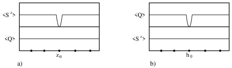
FIG. 2.: a) Profile of the spin- and charge-distribution of a localized spinon at $z_{\alpha}$; b) Profile of the spin- and charge-distribution of a localized holon at $h_{0}$.

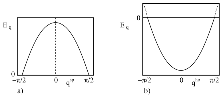
FIG. 3.: a) One-spinon dispersion relation; b) Negative-energy part of the one-holon dispersion relation.

Since spinons maintain their integrity, we can build multi-spinon states by first creating $M$-localized spinons and then by propagating each one of them. A residual spinon-interaction will require a further diagonalization of the Hamiltonian matrix restricted to the multi-spinon plane-wave subspace, as we will see in the particular case of two-spinon states.

To construct the state for two localized spinon at $z_{\alpha}$ and $z_{\beta}$, let us consider a HS-chain with even $N$. Let the $M(=N/2-1)$ spins at $z_{1},\ldots,z_{M}$ be $\uparrow$ and let the spin at $z_{\alpha}$ and $z_{\beta}$ be held $\downarrow$. The corresponding collective wavefunction will be given by:

$$\Psi_{\alpha\beta}^{\rm sp}(z_{1},\ldots,z_{M})=\prod_{j=1}^{M}(z_{j}-z_{\alpha})(z_{j}-z_{\beta})\prod_{i<j=1}^{M}(z_{i}-z_{j})^{2}\prod_{t=1}^{M}z_{t}$$ (13)

A set of independent two-propagating-spinon wavefunctions is given by the states:

$$\Psi_{mn}^{\rm sp}(z_{1},\ldots,z_{M})=\frac{1}{N^{2}}\sum_{\alpha=1}^{N}\sum_{\beta=1}^{N}(z_{\alpha}^{*})^{m}(z_{\beta}^{*})^{n}\Psi_{\alpha\beta}^{\rm sp}(z_{1},\ldots,z_{M})\;\;;\;m\geq n=0\ldots M$$ (14)

The Schrödinger equation for $\Psi_{\alpha\beta}^{\rm sp}$ now reads:

$\displaystyle{\cal H}_{\rm HS}\Psi^{\rm sp}_{\alpha\beta}=E_{\rm GS}\Psi^{\rm sp}_{\alpha\beta}+\frac{J}{2}\biggl{(}\frac{2\pi}{N}\biggr{)}^{2}\biggl{\{}-\frac{z_{\alpha}^{2}}{z_{\alpha}-z_{\beta}}\frac{\partial}{\partial z_{\alpha}}-\frac{z_{\beta}^{2}}{z_{\beta}-z_{\alpha}}\frac{\partial}{\partial z_{\beta}}-z_{\alpha}^{2}\frac{\partial^{2}}{\partial z_{\alpha}^{2}}-z_{\beta}^{2}\frac{\partial^{2}}{\partial z_{\beta}^{2}}$

$$+\biggl{(}\frac{N-3}{2}\biggr{)}\biggl{[}z_{\alpha}\frac{\partial}{\partial z_{\alpha}}+z_{\beta}\frac{\partial}{\partial z_{\beta}}\biggr{]}+[2M^{2}-M(N-2)]\biggr{\}}\Psi^{\rm sp}_{\alpha\beta}=\lambda\Psi^{\rm sp}_{\alpha\beta}$$ (15)

In the plane-wave basis, Eq.(15) becomes:

$\displaystyle\lambda\Psi_{mn}^{\rm sp}=\frac{J}{2}\biggl{(}\frac{2\pi}{N}\biggr{)}^{2}\biggl{\{}-\frac{N^{2}}{48}\biggl{(}N-\frac{19}{N}+\frac{24}{N^{2}}\biggr{)}$

$$+m(M-m)+n(M-n)-\frac{m-n}{2}\biggr{\}}\Psi_{mn}^{\rm sp}-\sum_{\ell=1}^{\ell_{M}}(m-n+2\ell)\Psi^{\rm sp}_{m+\ell,n-\ell}$$ (16)

where $\ell_{M}=n$ if $n+m<M$, $\ell_{M}=M-m$, if $n+m\geq M$. Eq.(16) has solutions of the form [13, 10]:

$$\Phi_{mn}^{\rm sp}=\sum_{\ell=0}^{\ell_{M}}a_{\ell}^{mn}\Psi^{\rm sp}_{m+\ell,n-\ell}$$ (17)

where the coefficients $a_{\ell}^{mn}$ are recursively defined as:

$$a_{\ell}^{mn}=-\frac{m-n+2\ell}{2\ell(\ell+m-n+\frac{1}{2})}\sum_{k=0}^{\ell-1}a_{k}^{mn}\;\;\;a_{0}^{mn}=1$$ (18)

The corresponding eigenvalues are given by:

$$E_{mn}=E_{\rm GS}+\frac{J}{2}\biggl{(}\frac{2\pi}{N}\biggr{)}^{2}\biggl{[}m(M-m)+n(M-n)-\frac{|m-n|}{2}\biggr{]}$$ (19)

Eq.(19) shows that the energy of the two spinons is equal to the ground state energy plus the energies of each single spinon plus an interaction contribution that is subleading in the thermodynamic limit. Indeed, as $N\rightarrow\infty$, we obtain:

$$E_{mn}-E_{\rm GS}\rightarrow E(q^{\rm sp}_{m},q^{\rm sp}_{n})=E(q^{\rm sp}_{m})+E(q^{\rm sp}_{n})$$ (20)

The fact that, in the thermodynamic limit, the energy is additive does not mean that the effects of spinon interaction disappear as $N\to\infty$. Instead, as we are going to see in the next Section, spinon interaction safely survives the thermodynamic limit, and appears to be the driving mechanism of the low-energy physics of one-dimensional antiferromagnets.

III Spinon dynamics in the Haldane-Shastry model

In this Section we study spinon interaction and its properties. To do so, we have to introduce a formalism that allows to treat spinons as actual quantum mechanical particles.

In Section II, we referred to the states $\Phi^{\rm sp}_{mn}$ as the two-spinon energy eigenstates, and to the states $\Psi^{\rm sp}_{\alpha\beta}$ as the states for two localized spinons at $z_{\alpha}$ and $z_{\beta}$. Therefore, it is always possible to fully decompose any of the $\Psi^{\rm sp}_{\alpha\beta}$’s within the set of the $\Phi^{\rm sp}_{mn}$’s:

$$\Psi_{\alpha\beta}^{\rm sp}=\sum_{m=0}^{M}\sum_{n=0}^{m}z_{\alpha}^{m}z_{\beta}^{n}{\cal P}_{mn}^{\rm sp}(\frac{z_{\beta}}{z_{\alpha}})\Phi^{\rm sp}_{mn}$$ (21)

where ${\cal P}_{mn}^{\rm sp}(z)$ is a polynomial in $z$ of degree $m-n$.

By definition, the coefficients of the combination in Eq.(21) provide the coordinate representation for the wavefunction for two spinons in a state of energy $E_{mn}$. The corresponding equation of motion for ${\cal P}_{mn}^{\rm sp}$ can be derived from the following identity chain (which is a direct consequence of Eq.(15)):

$\displaystyle E_{mn}\langle\Phi^{\rm sp}_{mn}|\Psi^{\rm sp}_{\alpha\beta}\rangle=\langle\Phi^{\rm sp}_{mn}|{\cal H}_{\rm HS}|\Psi^{\rm sp}_{\alpha\beta}\rangle$

$\displaystyle=E_{\rm GS}\langle\Phi^{\rm sp}_{mn}|\Psi^{\rm sp}_{\alpha\beta}\rangle+\rangle\frac{J}{2}\biggl{(}\frac{2\pi}{N}\biggr{)}^{2}\biggl{\{}(M-z_{\alpha}\frac{\partial}{\partial z_{\alpha}})z_{\alpha}\frac{\partial}{\partial z_{\alpha}}$

$$+(M-z_{\beta}\frac{\partial}{\partial z_{\beta}})z_{\beta}\frac{\partial}{\partial z_{\beta}}-\frac{1}{2}\biggl{(}\frac{z_{\alpha}+z_{\beta}}{z_{\alpha}-z_{\beta}}\biggr{)}\biggl{(}z_{\alpha}\frac{\partial}{\partial z_{\alpha}}-z_{\beta}\frac{\partial}{\partial z_{\beta}}\biggr{)}\biggr{\}}\langle\Phi^{\rm sp}_{mn}|\Psi^{\rm sp}_{\alpha\beta}$$ (22)

In the differential operator at the r.h.s. of Eq.(22) we recognize the energy operators of the two spinons, plus an interaction term that is velocity dependent and diverges as $1/x$ at short separation $x$ between the two particles.

From the equation $\langle\Phi^{\rm sp}_{mn}|\Psi^{\rm sp}_{\alpha\beta}\rangle$ = $\langle\Phi^{\rm sp}_{mn}|\Phi^{\rm sp}_{mn}\rangle z_{\alpha}^{m}z_{\beta}^{n}{\cal P}^{\rm sp}_{mn}(\frac{z_{\beta}}{z_{\alpha}})$ and from Eq.(22), we may derive the differential equation for the relative coordinate wavefunction:

$$\biggl{\{}z(1-z)\frac{d^{2}}{dz^{2}}+\biggl{[}\frac{1}{2}-m+n-(\frac{3}{2}-m+n)z\biggr{]}\frac{d}{dz}+\frac{m-n}{2}\biggr{\}}{\cal P}_{mn}^{\rm sp}(z)=0$$ (23)

Eq.(23) is a degenerate hypergeometric equation, with parameters $a=-m+n$, $b=1/2$, $c=a+b$. Its solution is provided by the hypergeometric polynomial [14]:

$${\cal P}_{mn}^{\rm sp}(z)={\cal P}_{m-n}^{\rm sp}(z)=\frac{\Gamma[m-n+1]}{\Gamma[\frac{1}{2}]\Gamma[m-n+\frac{1}{2}]}\sum_{k=0}^{m-n}\frac{\Gamma[k+\frac{1}{2}]\Gamma[m-n-k+\frac{1}{2}]}{\Gamma[k+1]\Gamma[m-n-k+1]}z^{k}$$ (24)

$|{\cal P}^{\rm sp}_{mn}(e^{ix})|^{2}$ gives the density of probability for the configuration with two spinons at a distance $x$, as a function of $x$. In Fig.4 we plot $|{\cal P}_{mn}^{\rm sp}(e^{ix})|^{2}$ vs. $x$. While at large separation the probability density oscillates and averages to 1, as it is appropriate for noninteracting particles, when the two spinons come close to each other, a huge probability enhancement appears utill the function reaches its maximum for $x=0$. The physical meaning of such a behavior may be summarized in two basic points:

• Spinon interaction is short ranged: This is clearly seen when the probability amplitude approaches the one for two noninteracting particles in the case when the spinons are far from each other;

• Spinon interaction is attractive: This is seen in the huge probability enhancement for configurations when the spinons are on top of each other.

Therefore, we have identified spinon interaction as a short range attraction. We now turn to the question of the fate of such an interaction in the thermodynamic limit. In order to do so, let us look at Fig.4b), where we show an insert of the plot of $|{\cal P}_{mn}^{\rm sp}(e^{ix})|^{2}$ around $x=0$, for the same relative momentum, but for increasing $N$. We see that, the larger $N$ is, the stronger the enhancement. Therefore, not only spinon interaction safely survives the thermodynamic limit but its effects become more relevant as the the sample size grows.

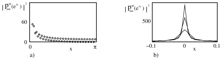
FIG. 4.: a) Square modulus of the two-spinon wavefunction for $N=100$ and $m-n\sim N/2-1$ as a function of spinon separation; b) Inset, at zero spinon separation, of the square modulus of the two-spinon wavefunction for increasing $N$. From bottom to top: $N=200,400,600$, respectively.

IV The Kuramoto-Yokoyama model of a one-dimensional insulator and its elementary excitations

In this Section we discuss the Kuramoto-Yokoyama (KY) model for a strongly correlated one-dimensional electron system. The KY-model is the supersymmetric extension of the HS-model. Strong on-site Coulomb repulsion forbids double occupancy, but one may have fewer electrons than sites. This allows for charged excitations (holes).

The Kuramoto-Yokoyama Hamiltonian is defined as [15]:

$\displaystyle{\cal H}_{\rm KY}=\frac{J}{2}\biggl{(}\frac{2\pi}{N}\biggr{)}^{2}\frac{1}{|z_{\alpha}-z_{\beta}|^{2}}P_{G}\biggl{\{}{\bf S}_{\alpha}\cdot{\bf S}_{\beta}-\frac{1}{2}\sum_{\sigma}c_{\alpha\sigma}^{\dagger}c_{\beta\sigma}+\frac{1}{2}(n_{\alpha}+n_{\beta})-\frac{n_{\alpha}n_{\beta}}{4}-\frac{3}{4}\biggr{\}}P_{G}$

where $c_{\alpha\sigma}$ is the single electron annihilation operator, $n_{\alpha}=\sum_{\sigma}c_{\alpha\sigma}^{\dagger}c_{\alpha\sigma}$ is the charge operator, and the Gutzwiller projector:

$\displaystyle P_{G}=\prod_{\alpha=1}^{N}(1-c_{\alpha\uparrow}^{\dagger}c_{\alpha\downarrow}^{\dagger}c_{\alpha\downarrow}c_{\alpha\uparrow})$

accounts for the no-double occupancy constraint.

In addition to the usual “bosonic” symmetry, generated by the total spin operator ${\bf S}$ and by the total charge operator $N=\sum_{\alpha}n_{\alpha}$, ${\cal H}_{\rm KY}$ also possesses four Fermionic symmetry operators, given by ${\cal Q}_{\sigma}=\sum_{\alpha=1}^{N}c_{\alpha\sigma}$ and by ${\cal Q}^{\dagger}_{\sigma}=\sum_{\alpha=1}^{N}c_{\alpha\sigma}^{\dagger}$ [9].

Exactly at half-filling, ${\cal H}_{\rm KY}$ reduces back to ${\cal H}_{\rm HS}$. Therefore, the ground state of ${\cal H}_{\rm KY}$ at half-filling is still given by $|\Psi_{\rm GS}\rangle$. Also, charge-0, spin-1/2 spinon excitations will be described by the same wavefunctions $\Psi_{\alpha}^{\rm sp}$ and $\Psi_{m}^{\rm sp}$ we have derived for one spinon in the HS-model, with the same dispersion relation.

A One-holon and one-holon one-spinon states of the KY-model

In order to construct charge-1, spin-0 holons, we may consider a state where one electron is removed from the top of a spinon, so that the resulting charge vacancy will carry no spin. The dispersion relation of such an excitation spans, in general, the whole Brillouin zone. Therefore, both positive- and negative-energy holons may arise, as charged excitations of the KY-model. Because of the supersymmetry of ${\cal H}_{\rm HS}$, a positive-energy holon state may be obtained by acting with ${\cal Q}_{\downarrow}$ on one-spinon fully polarized states. As those states will not be relevant for our analysis, we will neglect them in the following, and will rather focus onto wavefunctions with negative-energy holons.

In the case of odd $N$, the wavefunction for a propagating negative energy holon is given by:

$$\Psi_{n}^{\rm ho}(z_{1},\ldots,z_{M}|h)=h^{n}\prod_{j=1}^{N}(z_{j}-h)\prod_{i<j=1}^{N}(z_{i}-z_{j})^{2}\prod_{t=1}^{N}z_{t}\;\;;\;0\leq n\leq\frac{N+1}{2}$$ (25)

where $M=(N-1)/2$, and $z_{1},\ldots,z_{M}$ denote the position of the $\uparrow$-spin electrons. $h$ is the position of the empty site.

Clearly, $\Psi_{n}^{\rm ho}$ carries total charge 1. By using the technique introduced for the HS-model, it is straightforward to prove that $S^{z}\Psi_{n}^{\rm ho}=S^{-}\Psi_{n}^{\rm ho}=0$. Therefore, $S^{z}\Psi_{n}^{\rm ho}$ is a spin-0, charge-1 state, that is, a one-holon spin singlet.

The mathematical derivation of the action of ${\cal H}_{\rm KY}$ on $\Psi_{n}^{\rm ho}$ is long and boring, although straightforward. Here, we will not go through the various mathematical steps, but will rather quote the final result:

$\displaystyle[{\cal H}_{\rm KY}\Psi_{n}^{\rm ho}](z_{1},\ldots,z_{M}|h)=\biggl{\{}-J\biggl{(}\frac{\pi^{2}}{24}\biggr{)}\biggl{(}N-\frac{1}{N}\biggr{)}+\frac{J}{2}\biggl{(}\frac{2\pi}{N}\biggr{)}^{2}\;n(n-\frac{N+1}{2})\biggr{\}}\Psi_{n}^{\rm ho}(z_{1},\ldots,z_{M}|h)$

$$=\biggl{\{}-J\biggl{(}\frac{\pi^{2}}{24}\biggr{)}\biggl{(}N+\frac{5}{N}-\frac{3}{N^{2}}\biggr{)}+E(q_{n}^{\rm ho}))\biggr{\}}\Psi_{n}^{\rm ho}$$ (26)

In Eq.(26) we have introduced the one-holon crystal momentum, $q_{n}^{\rm ho}=\pi N/2+2\pi(n-1/4)/N$ $({\rm mod}\;2\pi)$, and the dispersion relation:

$$E(q_{n}^{\rm ho})=-\frac{J}{2}\biggl{[}(\frac{\pi}{2})^{2}-(q_{n}^{\rm ho})^{2}\biggr{]}$$ (27)

The negative-energy part of the dispersion relation in Eq.(27) is plotted in Fig.3(b). Again, one may recognize that the dispersion relation becomes gapless at the corners of the Brillouin zone, similarly to what happens for spinons. The remaining half-part of the Brillouine zone is spanned by positive-energy states, which we are not considering here.

The state for a localized holon at $h_{0}$, provided by the Fourier transform of $\Psi_{n}^{\rm ho}$ reads:

$$\Psi_{h_{0}}^{\rm ho}=\sum_{n=0}^{\frac{N+1}{2}}h_{0}^{-n}\Psi_{n}^{\rm ho}$$ (28)

Let us now introduce the one-spinon one-holon states of the KY-model. The starting point is provided by the states $\Psi_{n,s}^{\rm sp,ho}$, where the holon is propagating, while the spinon is localized at $s$. Let $N$ be even, $M=N/2-1$, and let:

$\displaystyle\Psi_{n,s}^{\rm sp,ho}(z_{1},\ldots,z_{M})=$

$$h^{n}\prod_{j=1}^{M}[(z_{j}-s)(z_{j}-h)]\prod_{i>j=1}^{M}(z_{i}-z_{j})^{2}\prod_{t=1}^{M}z_{t}\;\;;\;1\leq n\leq M+2$$ (29)

The KY-Hamiltonian acts on $\Psi_{n,s}^{\rm sp,ho}$ as follows [16, 17]:

$\displaystyle[\frac{{\cal H}_{\rm KY}}{\frac{J}{2}(\frac{2\pi}{N})^{2}}-E_{\rm GS}]\Psi_{n,s}^{\rm sp,ho}(z_{1},\ldots,z_{M})=$

$\displaystyle\biggl{\{}\biggl{(}n-M)+(M-1)s\frac{\partial}{\partial s}-s^{2}\frac{\partial^{2}}{\partial s^{2}}+\frac{1}{2}\frac{h+s}{h-s}\biggl{(}s\frac{\partial}{\partial s}+(1-n)\biggr{)}\biggr{\}}\Psi_{n,s}^{\rm sp,ho}$

$$+\frac{hs}{(h-s)^{2}}\biggl{(}\Psi_{n,s}^{\rm sp,ho}-\left(\frac{s}{h}\right)^{n-1}\Psi_{n,s=h}^{\rm sp,ho}\biggr{)}$$ (30)

In order to construct the corresponding energy eigenstates of ${\cal H}_{\rm KM}$, let us consider the one-spinon, one-holon plane waves:

$$\Psi_{mn}^{\rm sp,ho}(z_{1},\ldots,z_{M})=\sum_{s}\frac{(s^{*})^{m}}{N}\Psi_{n,s}^{\rm sp,ho}(z_{1},\ldots,z_{M})$$ (31)

In the plane wave basis, the eigenvalue equation takes the form:

$\displaystyle[\frac{{\cal H}_{\rm KY}}{\frac{J}{2}(\frac{2\pi}{N})^{2}}-E_{\rm GS}]\Psi_{mn}^{\rm sp,ho}=\biggl{[}m(M-m)+n(n-1+\frac{N}{2})\biggr{]}\Psi_{mn}^{\rm sp,ho}$

$$-\frac{1}{2}(n-m+1)\Psi_{mn}^{\rm sp,ho}-(n-m-1)\sum_{j=1}^{m}\Psi_{m-j,n+j}^{\rm sp,ho}$$ (32)

if $m-n+1<0$, and:

$\displaystyle[\frac{{\cal H}_{\rm KY}}{\frac{J}{2}(\frac{2\pi}{N})^{2}}-E_{\rm GS}]\Psi_{mn}^{\rm sp,ho}=\biggl{[}m(M-m)+n(n-1+\frac{N}{2})\biggr{]}\Psi_{mn}^{\rm sp,ho}$

$$-\frac{1}{2}(m-n+1)\Psi_{mn}^{\rm sp,ho}-(m-n+1)\sum_{j=1}^{M-m}\Psi_{m+j,n-j}^{\rm sp,ho}$$ (33)

if $m-n+1\geq 0$.

Eqs.(32,33) take the following eigenvectors and eigenvalues:

• Case $m-n+1<0$:

  
  

  $\displaystyle\Phi_{mn}^{\rm sp,ho}=\sum_{j=0}^{m}(-1)^{j}\frac{\Gamma[j+\frac{1}{2}]}{\Gamma[\frac{1}{2}]\Gamma[j+1]}\Psi^{\rm sp,ho}_{m-j,n+j}$

  $$E_{mn}^{+}=E_{\rm GS}+\frac{J}{2}\biggl{(}\frac{2\pi}{N}\biggr{)}^{2}\biggl{[}m(M-m)+n(n-1-\frac{N}{2})-\frac{1}{2}(n-m-1)\biggr{]}$$ (34)

• Case $m-n+1\geq 0$:

  
  

  $\displaystyle\Phi^{\rm sp,ho}_{mn}=\sum_{j=0}^{M-m}(-1)^{j}\frac{\Gamma[j+\frac{1}{2}]}{\Gamma[\frac{1}{2}]\Gamma[j+1]}\Psi^{\rm sp,ho}_{m+j,n-j}$

  $$E_{mn}^{-}=E_{\rm GS}+\frac{J}{2}\biggl{(}\frac{2\pi}{N}\biggr{)}^{2}\biggl{[}m(M-m)+n(n-1-\frac{N}{2})+\frac{1}{2}(n-m-1)\biggr{]}$$ (35)

Notice that, in either case, the energy can be written in terms of the spinon and holon momenta as:

$$E_{mn}=E_{\rm GS}+E(q_{m}^{\rm sp})+E(q_{n}^{\rm ho})-\frac{\pi J}{N}|q_{m}^{\rm sp}-q_{n}^{\rm ho}|$$ (36)

From Eq.(36) we see that, as for the case of two spinons, in the thermodynamic limit the energy of a spinon-holon pair on top of the ground state energy reduces to the sum of the energies of the single isolated spinon and of the single isolated holon. As for spinons, this does not imply the interaction between spinons and holons has no effects as the size of the system goes large.

V One-spinon one-holon dynamics in the Kuramoto-Yokoyama model

In order to write down the Schrödinger equation for a spinon-holon pair, Eq.(23), in analogy with two spinons, we need to define the state of a localized spinon at $s$ and a localized anyon at $h_{0}$. Fourier transforming $\Psi_{n,s}^{\rm sp,ho}$ back to coordinate space performs this task:

$$\Psi_{s,h_{0}}^{\rm sp,ho}(z_{1},\ldots,z_{M})=\sum_{n=1}^{M+2}h_{0}^{-n}\Psi_{n,s}^{\rm sp,ho}$$ (37)

$\Psi_{s,h_{0}}^{\rm sp,ho}$ can be fully decomposed within the basis of one-spinon, one-holon energy eigenstates. In particular, we obtain:

$$\Psi_{s,h_{0}}^{\rm sp,ho}=\sum_{n=1}^{M+2}\sum_{m=0}^{n-2}s^{m}h_{0}^{-n}{\cal P}^{\rm sp,ho}_{mn}(\frac{s}{h_{0}})\Phi^{\rm sp,ho}_{mn}+\sum_{n=1}^{M+2}\sum_{m=n-1}^{M}s^{m}h_{0}^{-n}{\cal P}^{\rm sp,ho}_{mn}(\frac{s}{h_{0}})\Phi^{\rm sp,ho}_{mn}$$ (38)

Eq.(38) defines the one-spinon one-holon relative wavefunction ${\cal P}_{mn}^{\rm sp,ho}$. To write down the equation of motion for the one-spinon one-holon wavefunction, we need the string of identities:

$\displaystyle(E_{mn}^{(\pm)}-E_{\rm GS})\langle\Phi_{mn}^{\rm sp,ho}|\Psi_{s,h_{0}}^{\rm sp,ho}\rangle=\langle\Phi_{mn}^{\rm sp,ho}|(\frac{{\cal H}_{\rm KY}}{\frac{J}{2}(\frac{2\pi}{N})^{2}}-E_{\rm GS})|\Psi_{s,h_{0}}^{\rm sp,ho}\rangle=$

$\displaystyle\biggl{\{}(M-s\frac{\partial}{\partial s})s\frac{\partial}{\partial s}+(\frac{N}{2}+1+h_{0}\frac{\partial}{\partial h_{0}})h_{0}\frac{\partial}{\partial h_{0}}+\frac{1}{2}\biggl{(}\frac{h_{0}+s}{h_{0}-s}\biggr{)}\biggl{(}s\frac{\partial}{\partial s}+h_{0}\frac{\partial}{\partial h_{0}}+1\biggr{)}\biggr{\}}\langle\Phi_{mn}^{\rm sp,ho}|\Psi_{s,h_{0}}^{\rm sp,ho}\rangle$

$$+\frac{h_{0}}{s-h_{0}}\biggl{(}\frac{s}{h_{0}}\biggr{)}^{\nu}\langle\Phi_{mn}^{\rm sp,ho}|\Psi_{s,h_{0}}^{\rm sp,ho}\rangle$$ (39)

where $\nu=M$ if $m-n+1<0$, $\nu=0$ otherwise.

From Eq.(39), it is straightforward to derive the differential equation for ${\cal P}_{mn}^{\rm sp,ho}$:

$\displaystyle\biggl{[}2\frac{d}{dz}-\frac{1}{(1-z)}\biggr{]}{\cal P}^{\rm sp,ho}_{mn}(z)+\frac{z^{M-m+1}}{(1-z)}{\cal P}^{\rm sp,ho}_{mn}(z)=0$

if $m-n+1<0$, and:

$$\biggl{[}2\frac{d}{d(\frac{1}{z})}-\frac{1}{(1-\frac{1}{z})}\biggr{]}{\cal P}^{\rm sp,ho}_{mn}(z)+\frac{(\frac{1}{z})^{m}}{(1-\frac{1}{z})}{\cal P}^{\rm sp,ho}_{mn}(z)=0$$ (40)

if $m-n+1\geq 0$.

Notice that, unlike the spinon case, Eqs.(40) are first-order differential equations. The reason for this is that spinon and holon energy bands have opposite curvature and, because of supersymmetry, the second derivatives of the dispersion relation have equal absolute values, but opposite signs. Nevertheless, one-spinon one-holon dynamics is basically the same as two-spinon dynamics, as we are going to discuss next.

Let us solve Eqs.(40). It is easy to see that they allow for polynomial-like solutions, given by:

$\displaystyle{\cal P}_{mn}^{\rm sp,ho}(z)=\sum_{k=0}^{M-m-1}\frac{\Gamma[k+\frac{1}{2}]}{\Gamma[\frac{1}{2}]\Gamma[k+1]}z^{k}\;\;\;(m-n+1<0)$

and:

$${\cal P}_{mn}^{\rm sp,ho}(z)=\sum_{k=0}^{m}\frac{\Gamma[k+\frac{1}{2}]}{\Gamma[\frac{1}{2}]\Gamma[k+1]}(\frac{1}{z})^{k}\;\;\;(m-n+1\geq 0).$$ (41)

The squared modulus of ${\cal P}^{\rm sp,ho}_{mn}(e^{ix})$ gives the probability of finding a spinon and a holon at a distance $x$ from each other. Such a probability is plotted in Fig.5a). Notice that, as for a spinon pair, at large separations between the two particles, the probability oscillates and averages to 1 flatly. This is a signal of the absence of long-range interaction effects. As the two particles get close one to each other, on the other hand, the probability peaks up, and shows a consistent enhancement at zero separation.

Therefore an interaction between spinons and holons exists. Such an interaction is short-ranged and, since it favors configurations with the two particles on top of each other, it is attractive. In conclusion, we assert that, as it happens among spinons, there is a short-range attraction as a relevant interaction between spinons and holons. The physical consequences of such an attraction is the subject of the next Section.

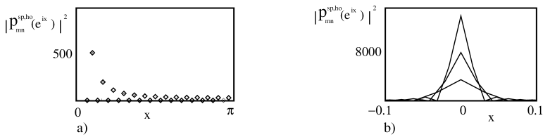
FIG. 5.: a) Square modulus of the one-spinon one-holon wavefunction for $N=100$ and $m-n\sim N/2-1$ as a function of spinon-holon separation; b) Inset at zero spinon-holon separation of the square modulus of the one-spinon one-holon wavefunction for increasing $N$. From bottom to top: $N=100,200,400$, respectively.

VI Physical consequences of the interaction between spinons and holons

In this Section we address the question of how spinon-spinon and spinon-holon interaction can be seen in a real experiment.

The experiments we think about are neutron scattering measurements performed on quasi one-dimensional antiferromagnets [5], and ARPES spectra measurements, performed on quasi one-dimensional insulators [6]. In the former case, one measures the dynamical spin form factor, that is, the imaginary part of the spin susceptibility, defined as:

$\displaystyle{\cal A}^{\rm spin}(\omega,q)=\frac{1}{3}\Im m\{\langle\Psi_{\rm GS}|{\bf S}(-\omega,-q)\cdot{\bf S}(\omega,q)|\Psi_{\rm GS}\rangle\}$

In the latter case, on the other hand, the photoemission of an electron from the sample is induced and, by detecting the emitted photoelectron, one eventually reconstructs the spectral function of the recoiling photohole, defined as:

$\displaystyle{\cal A}^{\rm hole}(\omega,q)=\frac{1}{\pi}\Im m\{G_{\rm hole}(\omega,q)\}$

where $G_{\rm hole}(\omega,q)$ is the hole Green function.

By using the results we derived in the previous Section, we can exactly calculate the contribution to ${\cal A}^{\rm spin}(\omega,q)$ from two spinon states, as well as the contribution to ${\cal A}^{\rm hole}(\omega,q)$ coming from one-spinon one-holon states, ${\cal A}^{\rm sp,ho}(\omega,q)$. In particular, we can express these contributions in terms of the two-spinon and of the one-spinon one-holon wavefunctions, calculated when the two particles are on top of each other. In this way, we directly see what the measurable consequences of the probability enhancement (and therefore the interaction between particles) are.

The wavefunction for propagating spin-one excitation with momentum $q=2\pi k/N$ is given by:

$$S_{q}^{-}\Psi_{\rm GS}=\sum_{\alpha}(z_{\alpha}^{*})^{k}\Psi_{\alpha\alpha}^{\rm sp}=N\sum_{m=0}^{N}\sum_{n=0}^{m}(-1)^{m+n}z_{\alpha}^{m+n}\delta(n+m-k){\cal P}^{\rm sp}_{mn}(1)\Phi_{mn}^{\rm sp}$$ (42)

Therefore, the form factor will be:

$\displaystyle{\cal A}^{\rm sp}(\omega,q)=2N^{2}\Im m\biggl{\{}\sum_{m=0}^{N}\sum_{n=0}^{m}\frac{\langle\Phi_{mn}^{\rm sp}|\Phi_{mn}^{\rm sp}\rangle}{\langle\Psi_{\rm GS}|\Psi_{\rm GS}\rangle}\times$

$$[{\cal P}_{mn}^{\rm sp}(1)]^{2}\delta(n+m-k)\frac{E_{mn}-E_{\rm GS}}{(\omega+i0^{+})^{2}-(E_{mn}-E_{\rm GS})^{2}}\biggr{\}}$$ (43)

From Eq.(43) we see that ${\cal A}^{\rm sp}(\omega,q)$ is fully determined only by the squared modulus of the two-spinon wavefunctions at zero separation between the two spinons, that is, by the probability enhancement. Since the probability enhancement is a direct consequence of spinon attraction, we get to the ultimate result that the spin form factor in one-dimensional antiferromagnets is fully determined only by spinon attraction.

An expression similar to Eq.(43) holds for ${\cal A}^{\rm sp,ho}(\omega,q)$. In particular, we obtain [16, 17]:

$\displaystyle{\cal A}^{\rm sp,ho}(\omega,q)=\Im m\frac{1}{\pi}\biggl{\{}\sum_{l=1}^{M+2}\sum_{m=0}^{l-2}\frac{\delta(k-m+l)[{\cal P}_{mn}^{\rm sp,ho}(1)]^{2}}{\omega+i0^{+}-(E^{+}_{mn}-E_{\rm GS})}$

$$+\sum_{l=1}^{M+2}\sum_{m=l-1}^{M}\frac{\delta(k-m+l)[{\cal P}_{mn}^{\rm sp,ho}(1)]^{2}}{\omega+i0^{+}-(E^{-}_{mn}-E_{\rm GS})}$$ (44)

where, again, we see that the one-spinon one-holon contribution to the hole spectral function is entirely determined only by the probability enhancement, that is, by spinon-holon attraction.

The relevant quantities appearing in Eqs.(43,44) are the squared modulus of the wavefunctions when the two particles are on top of each other, and the norms of the many-body two-spinon and one-spinon one-holon states. The values of those quantities are reported in Appendix A, where we show that they are basically given by products and ratios of Euler’s $\Gamma$-functions. Therefore, taking the thermodynamic limit of Eqs.(43,44) is just matter of properly using Stirling’s approximation:

$\displaystyle\Gamma[z]\approx\sqrt{\pi}(z-1)^{z-\frac{1}{2}}e^{-(z-1)}\;\;\;(z\;{\rm large})$

As discussed in detail in Refs.[10, 17], the final result is:

$${\cal A}^{\rm spin}(\omega,q)=\frac{J}{4}\frac{\Theta[\omega_{2}(q)-\omega]\Theta[\omega-\omega_{+1}(q)]\Theta[\omega-\omega_{-1}(q)]}{\sqrt{[\omega-\omega_{-1}(q)]}\sqrt{[\omega-\omega_{+1}(q)]}}$$ (45)

(where $\omega_{-1}(q)=J/2q(\pi-q)$, $\omega_{+1}(q)=J/2(2\pi-q)(q-\pi)$, and $\omega_{2}(q)=J/2q(2\pi-q)$), for the spin form factor, and:

$${\cal A}^{\rm sp,ho}(\omega,q)=\frac{1}{\pi^{2}Jq}\sqrt{\frac{J[q+\frac{\pi}{2}]^{2}-\omega}{\omega-J[q-\frac{\pi}{2}]^{2}}}$$ (46)

for the one-spinon, one-holon contribution to the hole spectral density.

The quantities reported in Eqs.(45,46) share some important features. Indeed, we see that no resonances appear in either case. A resonance would be an evidence for a stable spin-one propagating spin-wave in the former case, and for a stable propagating hole state in the latter case. We rather see broad features at the tails of the spectra, basically signaling the nonintegrity of the spin-wave versus decay into a spinon pair, and of the hole versus decay into a spinon-holon pair. Moreover, the spectra take sharp spikes at the creation threshold, that is, when the two-spinon/spinon-holon pair is created at the minimum of energy. Such a sharp threshold appears quite a natural consequence of our results, that is, it is the effect of the attraction, taken in the thermodynamic limit.

Sharp threshold features have been seen in the experiments quoted above [5, 6]. They should be interpreted as a direct experimental evidence of attraction among spinons and spinons and holons. Such an attraction appears to be ubiquitous for fractionalized excitations in one-dimensional strongly correlated systems, despite the fact that we have derived it within the framework of a somehow oversimplified mathematical model.

VII Conclusion

In these notes we have reviewed some results concerning the interaction among collective excitations of strongly correlated one-dimensional electronic systems: holons and spinons. A detailed mathematical derivation, performed within the framework of the Haldane-Shastry and of the Kuramoto-Yokoyama model, the simplest models of one-dimensional antiferromagnet and of one-dimensional strongly correlated insulator, provided us with important informations about such an interaction and its nature. We have seen that two spinons, as well as a spinon and a holon, interact by means of a short-range attraction. Although such an attraction creates a probability enhancement that goes large in the thermodynamic limit, it is not able to create a two-spinon or a one spinon-one holon bound state (a propagating spin wave or a propagating hole, respectively). The effect of the attraction is rather the creation of a sharp emission threshold in the spin-wave and in the hole spectral function, on top of a broad two-spinon, or one-spinon one-holon continuum. Such a sharp threshold is seen in neutron scattering experiment on quasi one-dimensional antiferromagnets [5], and in ARPES spectra measurements on quasi-one-dimensional insulator. In our view, it provides relevant evidence for an attractive interaction between spinons, and between spinons and holons.

A Norms and probability enhancements

In this Appendix we provide the formulas for the norms of two-spinon and one-spinon, one-holon states and for the two-spinon and one-spinon, one-holon probability enhancements. We will skip the long and boring, though straightforward, mathematical derivation of the results of this Appendix, and refer the interested reader to the original papers [10, 17].

The starting point for the derivation of $\langle\Phi_{mn}^{\rm sp}|\Phi_{mn}^{\rm sp}\rangle$ is a formula derived by K. Wilson [18]:

$$(\frac{N}{2\pi i})^{M}\oint\frac{dz_{1}}{z_{1}}\ldots\oint\frac{dz_{M}}{z_{M}}\prod_{i\neq j=1}^{M}(1-\frac{z_{i}}{z_{j}})^{2}=N^{M}\frac{(2M)!}{2^{M}}$$ (A1)

The next step is to consider the recursion relations

$\displaystyle\frac{\langle\Phi_{mn}^{\rm sp}|\Phi_{mn}^{\rm sp}\rangle}{\langle\Phi_{m-1,n}^{\rm sp}|\Phi_{m-1,n}^{\rm sp}\rangle}=\frac{(n-\frac{1}{2})(M-n+\frac{3}{2})(m-n+1)^{2}}{n(M-n+1)(m-n+\frac{3}{2})(m-n+\frac{1}{2})}$

and:

$$\frac{\langle\Phi_{mn}^{\rm sp}|\Phi_{mn}^{\rm sp}\rangle}{\langle\Phi_{m,n-1}^{\rm sp}|\Phi_{m,n-1}^{\rm sp}\rangle}=\frac{(M-m+1)(m-n+\frac{1}{2})(m-n-\frac{1}{2})m}{(M-m+\frac{1}{2})(m+\frac{1}{2})(m-n)^{2}}$$ (A2)

Eqs.(A2) are solved by:

$\displaystyle\langle\Phi_{mn}^{\rm sp}|\Phi_{mn}^{\rm sp}\rangle=C_{M}\frac{\Gamma[m-n+\frac{1}{2}]\Gamma[m-n+\frac{3}{2}]}{\Gamma^{2}[m-n+1]}\frac{\Gamma[m+1]\Gamma[M-m+\frac{1}{2}]}{\Gamma[m+\frac{3}{2}]\Gamma[M-m+1]}\times$

$$\frac{\Gamma[n+\frac{1}{2}]\Gamma[M-n+1]}{\Gamma[n+1]\Gamma[M-n+\frac{3}{2}]}$$ (A3)

where $C_{M}$ may be calculated from Wilson’s integral in Eq.(A1), and is given by $C_{M}=N^{M}(2M)!(M+\frac{1}{2})/(\pi 2^{M})$.

A similar technique may be applied, to derive $\langle\Phi_{mn}^{\rm sp,ho}|\Phi_{mn}^{\rm sp,ho}\rangle$. The result is:

$\displaystyle\langle\Phi_{mn}^{\rm sp,ho}|\Phi_{mn}^{\rm sp,ho}\rangle=N^{M+1}\frac{(2M)!}{2^{M}}(M+\frac{1}{2})\frac{\Gamma[M-m+1]\Gamma[m+\frac{1}{2}]}{\Gamma[M-m+\frac{3}{2}]\Gamma[m+1]}$

for $m-n+1<0$, and:

$$\langle\Phi_{mn}^{\rm sp,ho}|\Phi_{mn}^{\rm sp,ho}\rangle=N^{M+1}\frac{(2M)!}{2^{M}}(M+\frac{1}{2})\frac{\Gamma[M-m+\frac{1}{2}]\Gamma[m+1]}{\Gamma[M-m+1]\Gamma[m+\frac{3}{2}]}$$ (A4)

for $m-n+1\geq 0$.

The probability enhancement ${\cal P}_{mn}^{\rm sp}(1)$ may be derived from standard properties of hypergeometric functions [14]. The result is:

$${\cal P}_{mn}^{\rm sp}(1)=\frac{\Gamma[\frac{1}{2}]\Gamma[m-n+1]}{\Gamma[m-n+\frac{1}{2}]}$$ (A5)

Finally, ${\cal P}_{mn}^{\rm sp,ho}(1)$ may be recursively derived, as discussed in the Appendix of Ref.[17], and the result is:

$\displaystyle{\cal P}_{mn}^{\rm sp,ho}(1)=2\frac{\Gamma[M-m+\frac{1}{2}]}{\Gamma[\frac{1}{2}]\Gamma[M-m]}$

for $m-n+1<0$, and:

$${\cal P}_{mn}^{{\rm sp,ho}}(1)=2\frac{\Gamma[m+\frac{3}{2}]}{\Gamma[\frac{1}{2}]\Gamma[m+1]}$$ (A6)

for $m-n+1\geq 0$.

- [1] L. D. Landau, Sov. Phys. JETP 3, 920(1957); Sov. Phys. JETP 5, 101(1957) Sov. Phys. JETP 8, 70(1958).
- [2] J. des Cloizeaux and J. J. Pearson, Phys. Rev. 128, 2131 (1962).
- [3] L. D. Fadeev and L. A. Takhtajan, Russian Math. Surveys 34, 11 (1979).
- [4] H. A. Bethe, Z. Physik 71, 205 (1931).
- [5] D. A. Tennant et al, Phys. Rev.B 60, 13368 (1995); R. Coldea et al., Phys. Rev. Lett. 79. 151 (1997); R. Coldea, Journal of Magnetism and Magnetic Materials, vol.177-181, 659 (1998).
- [6] C. Kim et al., Phys. Rev. B 56, 15589 (1997).
- [7] F. D. M. Haldane, Phys. Rev. Lett. 60, 635 (1988).
- [8] B. S. Shastry, Phys. Rev. Lett. 60, 639 (1988).
- [9] R. B. Laughlin, D. Giuliano, R. Caracciolo and O. White Field Theory for Low-Dimensional Systems, eds. G. Morandi, P. Sodano, A. Tagliacozzo and V. Tognetti (Springer, Heidelberg, 1999).
- [10] B. A. Bernevig, D. Giuliano and R. B. Laughlin, Phys. Rev. B 64, 024425 (2001).
- [11] B. S. Shastry, Phys. Rev. Lett. 69, 1153 (1992).
- [12] F. D. M. Haldane, Phys. Rev. Lett. 50, 1153 (1983); Phys Lett A93, 464 (1983).
- [13] B. A. Bernevig, D. Giuliano and R. B. Laughlin, Phys. Rev. Lett. 86, 3392 (2001).
- [14] M. Abramowitz, Handbook of Mathematical Functions, (United States. National Bureau of Standards. Applied mathematics series, 55, 1964).
- [15] Y. Kuramoto and M. Yokoyama, Phys. Rev. Lett. 67, 1338 (1991).
- [16] B. A. Bernevig, D. Giuliano and R. B. Laughlin, Phys. Rev. Lett. 87, 177206 (2001).
- [17] A. Bernevig, D. Giuliano and R. B. Laughlin, Phys. Rev. B 65, 195112 (2002).
- [18] K. G. Wilson, Jour. Mat. Phys. 3, 1040 (1962).