Ground-state phases in a system of two competing square-lattice Heisenberg antiferromagnets

Abstract

We study a two-dimensional (2D) spin-half Heisenberg model related to the quasi 2D antiferromagnets $(Ba,Sr)_{2}Cu_{3}O_{4}Cl_{2}$ by means of exact diagonalization and spin-wave theory. The model consists of two inequivalent interpenetrating square-lattice Heisenberg antiferromagnets $A$ and $B$. While the antiferromagnetic interaction $J_{AA}$ within the $A$ subsystem is strong the coupling $J_{BB}$ within the $B$ subsystem is much weaker. The coupling $J_{AB}$ between A and B subsystems is competing giving rise for interesting frustration effects. In dependence of the strength of $J_{AB}$ we find a collinear Néel phase, non-collinear states with zero magnetizations as well as canted and collinear ferrimagnetic phases with non-zero magnetizations. For not too large values of frustration $J_{AB}$, which correpond to the situation in $(Ba,Sr)_{2}Cu_{3}O_{4}Cl_{2}$, we have Néel ordering in both subsystems A and B. In the classical limit these two Néel states are decoupled. Quantum fluctuations lead to a fluctuational coupling between both subsystems (’order from disorder’) and select the collinear structure. For stronger $J_{AB}$ we find evidence for a novel spin state with coexisting Néel ordering in the $A$ subsystem and disorder in the $B$ subsystem.

I Introduction

The exciting collective magnetic properties of layered cuprates have attracted much attention over the last decade. A lot of activity in this field was stimulated by the possible connection of spin fluctuations with the phenomenon of high-temperature superconductivity. But, the rather unusual properties of quantum magnets deserve study on their own to gain a deeper understanding of these quantum many-body systems. In recent years some of those materials such as $Ba_{2}Cu_{3}O_{4}Cl_{2}$ and $Sr_{2}Cu_{3}O_{4}Cl_{2}$ have been studied experimentally and theoretically in more detail [1, 2, 3, 4, 5]. The most important difference between $(Ba,Sr)_{2}Cu_{3}O_{4}Cl_{2}$ and their parent compound $La_{2}CuO_{4}$ is the existence of additional $Cu(B)$-atoms located at the centre of every second $Cu(A)$-plaquette. Both subsystems $A$ and $B$ form square lattices, however, with different orientations and lattice constants. This A-B lattice is illustrated in Fig.1a. Both copper sites $Cu(A)$ and $Cu(B)$ carry spin half, i.e. quantum fluctuations are important. Since the magnetic couplings $J_{AA}$ between A spins as well as $J_{BB}$ between B spins are antiferromagnetic and the coupling $J_{AB}$ between A and B spins is frustrating we have a system of two competing antiferromagnetic spin-half subsystems.

Three-dimensional examples of two interpenetrating antiferromagnets like garnets $Mn_{3}Cr_{2}Ge_{3}O_{12}$ or $(Fe_{x}Ga_{1-x})_{2}Ca_{3}Ge_{3}O_{12}$ were discussed by several authors (see e.g. [6, 7, 8]). For the quasi two-dimensional cuprates like $(Ba,Sr)_{2}Cu_{3}O_{4}Cl_{2}$ the quantum fluctuations are more important than in the three-dimensional garnets and the interplay of competing interactions with strong quantum fluctuations may lead to interesting magnetic phenomena.

Noro et al. [1] reported two magnetic phase transitions at $T_{A}=320K$ and at $T_{B}=40K$ for $Ba_{2}Cu_{3}O_{4}Cl_{2}$ being attributed to respective antiferromagnetic ordering of the $Cu(A)$ and $Cu(B)$ spins. Both critical temperatures differ in one order of magnitude indicating a strongly antiferromagnetic coupling between $Cu(A)$ spins and a comparatively small antiferromagnetic coupling between $Cu(B)$ spins, which is confirmed by band-structure calculations [9]. According to Chou et al. [3] the weak ferromagnetic moment found experimentally [2] could be understood as a consequence of bond-dependent interactions such as pseudodipolar couplings.

The minimal model to describe the main magnetic properties of the competing antiferromagnets on the A-B lattice is the antiferromagnetic Heisenberg model with three exchange couplings $J_{AA}$, $J_{BB}$ and $J_{AB}$. In what follows we call this model A-B model. Some preliminary results for a finite system of ${\cal N}=24$ sites were reported in the conference paper [10]. However, to describe the weak ferromagnetism observed in these compounds anisotropic interactions seem to be needed [3, 4, 5].

In this paper we want to study the influence of strong quantum fluctuations and frustration on the ground state of the A-B model using spin-wave theory and exact diagonalization. The paper is organized as follows: In Section II we introduce the A-B model and illustrate the classical magnetic ground-state phases in the considered parameter region. In Section III we present an exact-diagonalization study of the ground-state phases and in Section IV the linear spin-wave approach is used to analyse the Néel phase realized for small $J_{AB}$ in more detail. In Section V a summary is given.

II The A-B model and its classical ground-state phases

We consider the Hamiltonian (cf. Fig. 1b)

$$H=J_{AA}\sum_{\left\langle m\in A,\,n\in A\right\rangle}{\bf{S}}_{m}\cdot{\bf{S}}_{n}+J_{BB}\sum_{\left\langle m\in B,\,n\in B\right\rangle}{\bf{S}}_{m}\cdot{\bf{S}}_{n}+J_{AB}\sum_{\left\langle m\in A,\,n\in B\right\rangle}{\bf{S}}_{m}\cdot{\bf{S}}_{n},$$ (1)

where the sums run over neighbouring sites only. $J_{AA}$ and $J_{BB}$ denote the antiferromagnetic couplings within the $A(B)$-subsystems, respectively. We focus our discussion on parameters $J_{AA}=1$ and $J_{BB}=0.1$ which corresponds to the situation in $(Ba,Sr)_{2}Cu_{3}O_{4}Cl_{2}$. The value of the frustrating inter-subsystem coupling $J_{AB}$ is less reliably known. We consider antiferromagnetic $J_{AB}$ and use it as the free parameter of the model. The lattice consists of ${\cal N}=3N$ spins with three spins per geometrical unit cell and ten couplings in it.

We start with the discussion of the classical ground state, i.e. the spins ${\bf{S}}_{n}$ are considered as classical vectors of length $s$. Varying $J_{AB}$ we have altogether five ground-state phases, see table I. Two of them (I and III) have planar spin arrangement, two (II and IV) are non-planar and one (V) is collinear. Without loss of generality we choose in this section for the description of planar spin ordering the x-y plane. We start from weak inter-subsystem coupling $J_{AB}\stackrel{{\scriptstyle>}}{{\sim}}0$. Then we have Néel ordering in both subsystems (phase I, table I). These two classical Néel states shown in Fig.2 are decoupled and can rotate freely with respect to each other, i.e. the ground state is highly degenerated and this degree of freedom is parametrized by the angle $\varphi$. The corresponding magnetic unit cell contains six spins. (Thus, later in Section IV we have to introduce six different magnons in the spin-wave theory for this phase.)

At $J_{AB}=2\sqrt{J_{AA}J_{BB}}$ there is a first-order transition from the Néel phase I to the non-planar ground-state phase II. Phase II is illustrated in Fig.3. The corresponding magnetic unit cell contains 12 pins and is therefore twice as large as the magnetic unit cell of the Néel phase I. In this state we have eight different spin orientations characterized as follows

$${\bf{S}}^{II}_{A_{1}} = s\left(-\frac{\sqrt{2}}{2}\cos\left(\alpha\right),-\frac{\sqrt{2}}{2}\cos\left(\alpha\right),\sin\left(\pm\alpha\right)\right),$$ (2)

$${\bf{S}}^{II}_{A_{2}} = s\left(\frac{\sqrt{2}}{2}\cos\left(\alpha\right),\frac{\sqrt{2}}{2}\cos\left(\alpha\right),\sin\left(\pm\alpha\right)\right),$$ (3)

$${\bf{S}}^{II}_{A_{3}} = s\left(-\frac{\sqrt{2}}{2}\cos\left(\alpha\right),\frac{\sqrt{2}}{2}\cos\left(\alpha\right),-\sin\left(\pm\alpha\right)\right),$$ (4)

$${\bf{S}}^{II}_{A_{4}} = s\left(\frac{\sqrt{2}}{2}\cos\left(\alpha\right),-\frac{\sqrt{2}}{2}\cos\left(\alpha\right),-\sin\left(\pm\alpha\right)\right),$$ (5)

$${\bf{S}}^{II}_{B_{1}} = s\left(-1,0,0\right),\quad{\bf{S}}^{II}_{B_{2}}=s\left(0,-1,0\right),$$ (6)

$${\bf{S}}^{II}_{B_{3}} = s\left(1,0,0\right),\quad{\bf{S}}^{II}_{B_{4}}=s\left(0,1,0\right),$$ (7)

where $\alpha$ is given by $\alpha=\mbox{arcos}\left(J_{AB}/\sqrt{8}J_{AA}\right)$. Obviously neighbouring B spins are perpendicular to each other and consequently the energy $E_{II}$ is independent of $J_{BB}$ (see table I). The in-plane xy components of the A spins of neigboring spins are also perpendicular, however, there are finite off-plane z components. These off-plane components (proportional to $\sin\alpha$, see eq. (7)) decrease with $J_{AB}$ and become zero at $J_{AB}=2\sqrt{2}\;J_{AA}$, i.e. we have a second-order transition from the non-planar phase II to the planar phase III at this point. The spin orientations of phase III are given by eq. (7), too, but with the additional condition $\alpha=0$ (see Fig. 3). In phase III neighbouring $A$-spins as well as neighbouring $B$-spins are perpendicular to each other and consequently the energy depends on $J_{AB}$ only. All three phases I,II,III have a zero net magnetization $S_{total}=0$.

Further increasing $J_{AB}$ favours an antiparallel alignment of the A spins relative to the B spins and the planar phase III gives way to a non-planar phase IV where the in-plane xy components are aligned as in phases II and III (see Fig. 3). The off-plane z components in phase IV are given as $S^{z}_{n\in A}=+s\cos\theta$ for A spins and as $S^{z}_{n\in B}=-s\;\sqrt{1-A^{2}\sin^{2}\theta}$ for B spins. This phase IV can be denoted as canted ferrimagnet [11] and has a net magnetic moment $S_{A}$ in the A subsystem and $S_{B}$ in the B subsystem resulting in a finite total magnetic moment $S_{total}$

$$\frac{S^{IV}_{A}}{s2N}=\sqrt{1-\sin^{2}{\theta}}\;;\;\frac{S^{IV}_{B}}{sN}=\sqrt{1-A^{2}\sin^{2}{\theta}}\;;\;{S^{IV}_{total}}=\left|S_{A}-S_{B}\right|$$ (8)

with

$${\sin{\theta}}=\sqrt{\frac{1-\left(\frac{J_{AA}}{J_{AB}}+\frac{J_{AB}}{4J_{BB}}-\frac{1}{4}\sqrt{-24\frac{J_{AA}}{J_{BB}}+16\frac{J_{AA}^{2}}{J_{AB}^{2}}+\frac{J_{AB}^{2}}{J_{BB}^{2}}}\right)^{2}}{-3\frac{J_{AA}}{J_{BB}}+2\frac{J_{AA}^{2}}{J_{AB}^{2}}+\frac{J_{AB}^{2}}{8J_{BB}^{2}}+\left(\frac{3J_{AA}}{2J_{AB}}-\frac{J_{AB}}{8J_{BB}}\right)\sqrt{-24\frac{J_{AA}}{J_{BB}}+16\frac{J_{AA}^{2}}{J_{AB}^{2}}+\frac{J_{AB}^{2}}{J_{BB}^{2}}}}}$$ (9)

and

$$A=\frac{J_{AB}}{2\sqrt{2}J_{BB}}-\sqrt{2}\frac{J_{AA}}{J_{AB}}-\sqrt{-3\frac{J_{AA}}{J_{BB}}+2\frac{J_{AA}^{2}}{J_{AB}^{2}}+\frac{J_{AB}^{2}}{8J_{BB}^{2}}}.$$ (10)

This total moment increases with $J_{AB}$. The energy of phase IV is given by

$$\frac{E_{IV}}{s^{2}{\cal N}} = \frac{4}{3}J_{AA}\left(1-\sin^{2}\theta_{0}\right)+\frac{2}{3}J_{BB}\left(1-A^{2}\sin^{2}\theta_{0}\right)$$ (12)

$$-\frac{4}{3}J_{AB}\left(\frac{A}{\sqrt{2}}+\sqrt{\left(1-\sin^{2}\theta_{0}\right)\left(1-A^{2}\sin^{2}\theta_{0}\right)}\right)$$

The phase boundary of the second order phase transition between III and IV is given by

$$J^{III-IV}_{AB}=\sqrt{2}J_{AA}+\frac{J_{BB}}{\sqrt{2}}+\frac{1}{2}\sqrt{8J^{2}_{AA}+24J_{AA}J_{BB}+2J^{2}_{BB}}$$ (13)

and yields $J^{III-IV}_{AB}=3.099$ for $J_{AA}=1$ and $J_{BB}=0.1$.

Finally, for large $J_{AB}$ the A and B spins are fully polarized along the z axis, i.e. ${\bf S}_{n\in A}=(0,0,+s)$ and ${\bf S}_{n\in B}=(0,0,-s)$ and a collinear ferrimagnetic phase V is realized. The phase boundary of this second order phase transition between IV and V is given by

$$J^{IV-V}_{AB}=2J_{AA}+J_{BB}+\sqrt{4J^{2}_{AA}+J^{2}_{BB}}$$ (14)

leading to $J^{IV-V}_{AB}=4.102$ for $J_{AA}=1$ and $J_{BB}=0.1$.

III The quantum ground state - exact diagonalization

To discuss the influence of quantum fluctuations on the classical phases studied in the last section we use the Lanczos algorithm to calculate the quantum ground state of the Hamiltonian (1) for a finite lattice of ${\cal N}=24$ spins (Fig.4). Again we choose the parameters $J_{AA}=1$, $J_{BB}=0.1$ appropriate for $(Ba,Sr)_{2}Cu_{3}O_{4}Cl_{2}$ and consider $J_{AB}$ as the free parameter. For ${\cal N}=24$ sites we have $16$ $A$ spins and $8$ $B$ spins. Since the maximal magnetic unit cell of the classical ground states contains $12$ spins the ${\cal N}=24$ system has the full symmetry of the classical ground state in the considered parameter region. To reduce the Hilbert space we used all possible translational and point symmetries of the A-B lattice as well as spin inversion. The use of the symmetry allows to classify the different quantum ground states by their symmetry.

To compare classical and quantum ground-state phases we present the spin-spin correlations in Figs. 5, 6 and 7. The Néel phase I is present also in the quantum model. However, the quantum fluctuations lift the classical degeneracy and both subsystems couple. The fluctuational coupling is known as order from disorder effect [12, 7] and selects a collinear quantum state with a finite A-B spin correlation in the quantum Néel phase I (see Fig. 7). Moreover, the transition to phase II is shifted to higher values of $J_{AB}$ indicating that quantum fluctuations favour collinear versus non-collinear states (see e.g. [13]). The frustrating coupling weakens the A-A and B-B spin correlations in the Néel phase I; this weakening is stronger for the B-B correlations than for the A-A correlations. Hence, a disordered quantum ground state similar to the $J_{1}-J_{2}$ model [14, 15, 16, 17, 18] seems to be possible and will be discussed in more detail in next Section.

The quantum Néel phase gives way to a fairly complex spin state at $J_{AB}\approx 1.02$ up to $J_{AB}\approx 3.13$. This state is also a singlet $S=0$ as the quantum Néel state. The A-A and the A-B spin correlations of the quantum model follow qualitatively the classical curves (see Figs. 5 and 7). However, we see some jumps in the correlations connected with level crossings of ground states belonging to different lattice symmetries. Most likely these level crossings may be attributed to finite-size effects. The change of A-A and A-B correlations at $J_{AB}\approx 1.02$ is small. However, the B-B correlations change strongly at this point. Contrary to the classical model where the nearest-neighbour B-B correlation is zero and the next-nearest-neighbour B-B correlation is strongly antiferromagnetic. The corresponding correlations in the quantum model are both different from zero and are of the same order of magnitude. One could argue that quantum fluctuations favour planar versus non-planar arrangement of spins. This argument is supported by (i) the circumstance that there is a planar classical state of almost the same energy as the non-planar state having finite nearest-neighbour B-B correlations and (ii) by investigation of the so-called scalar chirality $W_{ijk}={\bf S}_{i}\cdot({\bf S}_{j}\times{\bf S}_{k})$ being nonzero only in non-planar states. This kind of order parameter was widely discussed for the $J_{1}-J_{2}$ model [14, 16]. We choose $j\in B$ as the running index and consider for $i,j,k$ sites forming an equilateral triangle like sites 1, 23, 24 in Fig. 4, i.e. we have $k=j+{\bf a}_{2}$ and $i=j+{\bf a}_{1}+\frac{1}{2}{\bf a}_{1}$. Then we use as order parameter (cf. [16])

$$W=\left(\frac{1}{N}\sum_{j\in B}\tau_{j}W_{ijk}\right)^{2}$$ (15)

where $\tau_{j}$ is a staggered factor being $+1$ on sublattice $B_{1}$ (i.e. sites 17, 19, 21, 23 in Fig. 4) and $-1$ on sublattice $B_{2}$ (i.e. sites 18, 20, 22, 24 in Fig. 4). As shown by Fig. 8 this chirality is indeed large in the classical nonplanar states but we do not see significantly enhanced chiral correlations in the quantum ground state.

Further increasing $J_{AB}$ leads to a transition from the complex singlet $S=0$ phase directly to an $S=2$ phase at $J_{AB}\approx 3.13$, which is the quantum counterpart to the classical canted ferrimagnetic phase IV. This transition is very close to the classical transition III-IV which is also a transition from zero $S_{total}$ to finite $S_{total}$.

The last transition is that to the collinear ferrimagnetic state with $S=4$ at $J_{AB}\approx 3.61$. This value is significantly smaller than the corresponding classical value, again indicating that quantum fluctuations favour collinear spin ordering leading to an enlarged stability region of the collinear ferrimagnetic phase. Notice, that the additional jump just before the last transition is attributed to a change in total spin $S$ from $S=2$ to $S=3$ corresponding to the increase of $S_{total}$ in the classical phase IV. One characteristics of both ferrimagnetic ($S>0$) phases are the positive correlations within a subsystem (see Figs. 5 and 6) but negative correlations between the subsystems (see Fig. 7).

IV Linear spin-wave theory for the Néel phase

The parameters for which the Néel phase I is realized most likely correspond to the situation in $(Ba,Sr)_{2}Cu_{3}O_{4}Cl_{2}$. Therefore we present a more detailed analysis of the magnetic ordering of this phase using a linear spin-wave theory. Within this approach we calculate the excitation spectrum, the order parameter as well as the spin-wave velocity.

As usual we perform Holstein-Primakoff transformation. Because the magnetic unit cell contains six spins we need at least six different types of magnons being distinguished by a running index as illustrated in (Fig.2). After transforming into the ${\bf{k}}$-space the Hamiltonian (1) reads

$$H=-4NJ_{AA}s^{2}-2NJ_{BB}s^{2}+\sum_{{\bf{k}}}H_{{\bf{k}}}$$

with

$$H_{{\bf{k}}} = 4J_{AA}s\left(a^{+}_{1{\bf{k}}}a_{1{\bf{k}}}+a^{+}_{2{\bf{k}}}a_{2{\bf{k}}}+a^{+}_{3{\bf{k}}}a_{3{\bf{k}}}+a^{+}_{4{\bf{k}}}a_{4{\bf{k}}}\right)+4J_{BB}s\left(a^{+}_{5{\bf{k}}}a_{5{\bf{k}}}+a^{+}_{6{\bf{k}}}a_{6{\bf{k}}}\right)$$ (16)

$$- J_{AA}s\left(\gamma_{1{\bf{k}}}\gamma_{2{\bf{k}}}+\gamma^{\ast}_{1{\bf{k}}}\gamma^{\ast}_{2{\bf{k}}}\right)\left(a^{+}_{1{\bf{k}}}a^{+}_{4-{\bf{k}}}+a^{+}_{2{\bf{k}}}a^{+}_{3-{\bf{k}}}+a_{1{\bf{k}}}a_{4-{\bf{k}}}+a_{2{\bf{k}}}a_{3-{\bf{k}}}\right)$$ (17)

$$- J_{AA}s\left(\gamma_{1{\bf{k}}}\gamma^{\ast}_{2{\bf{k}}}+\gamma^{\ast}_{1{\bf{k}}}\gamma_{2{\bf{k}}}\right)\left(a^{+}_{1{\bf{k}}}a^{+}_{3-{\bf{k}}}+a^{+}_{2{\bf{k}}}a^{+}_{4-{\bf{k}}}+a_{1{\bf{k}}}a_{3-{\bf{k}}}+a_{2{\bf{k}}}a_{4-{\bf{k}}}\right)$$ (18)

$$- J_{BB}s\left(\gamma^{2}_{1{\bf{k}}}+\gamma^{2}_{2{\bf{k}}}+\gamma^{\ast 2}_{1{\bf{k}}}+\gamma^{\ast 2}_{2{\bf{k}}}\right)\left(a^{+}_{5{\bf{k}}}a^{+}_{6-{\bf{k}}}+a_{5{\bf{k}}}a_{6-{\bf{k}}}\right)$$ (19)

$$+ J_{AB}s\left(g+1\right)\left(\gamma_{1{\bf k}}\left(a^{+}_{1{\bf{k}}}a_{6{\bf{k}}}+a_{2{\bf{k}}}a^{+}_{6{\bf{k}}}\right)+\gamma^{\ast}_{1{\bf k}}\left(a_{1{\bf{k}}}a^{+}_{6{\bf{k}}}+a^{+}_{2{\bf{k}}}a_{6{\bf{k}}}\right)\right)/2$$ (20)

$$+ J_{AB}s\left(g-1\right)\left(\gamma_{1{\bf k}}\left(a^{+}_{1{\bf{k}}}a^{+}_{6{-\bf{k}}}+a_{2{\bf{k}}}a_{6-{\bf{k}}}\right)+\gamma^{\ast}_{1{\bf k}}\left(a_{1{\bf{k}}}a_{6-{\bf{k}}}+a^{+}_{2{\bf{k}}}a^{+}_{6-{\bf{k}}}\right)\right)/2$$ (21)

$$+ J_{AB}s\left(g+1\right)\left(\gamma_{2{\bf k}}\left(a^{+}_{4{\bf{k}}}a_{5{\bf{k}}}+a_{3{\bf{k}}}a^{+}_{5{\bf{k}}}\right)+\gamma^{\ast}_{2{\bf k}}\left(a_{4{\bf{k}}}a^{+}_{5{\bf{k}}}+a^{+}_{3{\bf{k}}}a_{5{\bf{k}}}\right)\right)/2$$ (22)

$$+ J_{AB}s\left(g-1\right)\left(\gamma_{2{\bf k}}\left(a^{+}_{4{\bf{k}}}a^{+}_{5{-\bf{k}}}+a_{3{\bf{k}}}a_{5-{\bf{k}}}\right)+\gamma^{\ast}_{2{\bf k}}\left(a_{4{\bf{k}}}a_{5-{\bf{k}}}+a^{+}_{3{\bf{k}}}a^{+}_{5-{\bf{k}}}\right)\right)/2$$ (23)

$$- J_{AB}s\left(g-1\right)\left(\gamma_{1{\bf k}}\left(a^{+}_{2{\bf{k}}}a_{5{\bf{k}}}+a_{1{\bf{k}}}a^{+}_{5{\bf{k}}}\right)+\gamma^{\ast}_{1{\bf k}}\left(a_{2{\bf{k}}}a^{+}_{5{\bf{k}}}+a^{+}_{1{\bf{k}}}a_{5{\bf{k}}}\right)\right)/2$$ (24)

$$- J_{AB}s\left(g+1\right)\left(\gamma_{1{\bf k}}\left(a^{+}_{2{\bf{k}}}a^{+}_{5{-\bf{k}}}+a_{1{\bf{k}}}a_{5-{\bf{k}}}\right)+\gamma^{\ast}_{1{\bf k}}\left(a_{2{\bf{k}}}a_{5-{\bf{k}}}+a^{+}_{1{\bf{k}}}a^{+}_{5-{\bf{k}}}\right)\right)/2$$ (25)

$$- J_{AB}s\left(g-1\right)\left(\gamma_{2{\bf k}}\left(a^{+}_{3{\bf{k}}}a_{6{\bf{k}}}+a_{4{\bf{k}}}a^{+}_{6{\bf{k}}}\right)+\gamma^{\ast}_{2{\bf k}}\left(a_{3{\bf{k}}}a^{+}_{6{\bf{k}}}+a^{+}_{4{\bf{k}}}a_{6{\bf{k}}}\right)\right)/2$$ (26)

$$- J_{AB}s\left(g+1\right)\left(\gamma_{2{\bf k}}\left(a^{+}_{3{\bf{k}}}a^{+}_{6{-\bf{k}}}+a_{4{\bf{k}}}a_{6-{\bf{k}}}\right)+\gamma^{\ast}_{2{\bf k}}\left(a_{3{\bf{k}}}a_{6-{\bf{k}}}+a^{+}_{4{\bf{k}}}a^{+}_{6-{\bf{k}}}\right)\right)/2$$ (27)

and $\gamma_{n{\bf{k}}}=\exp\left(i{\bf{k}}{\bf{a}}_{n}/2\right)$. Here $N$ is the number of geometrical unit cells $N={\cal N}/3$. The vectors ${\bf{a}}_{n}$ are the unit vectors of the geometrical lattice: ${\bf{a}}_{1}=a\left(1,0\right)$ and ${\bf{a}}_{2}=a\left(0,1\right)$ and $a$ is the lattice constant (see Fig. 1a). $g$ is defined as $g=\cos\left(\varphi\right)$, where $\varphi$ parametrizes the angle between the Néel states of the classical subsystems A and B. Without any further calculation it is obvious that quantum fluctuations stabilize collinear ordering. According to the Hellmann-Feynman theorem [19] the relation $\partial E/\partial\lambda=\left\langle\partial H/\partial\lambda\right\rangle$ holds, where $H$ is a Hamiltonian depending on a parameter $\lambda$ and $E$ is an eigenvalue of $H$. Because (LABEL:eq6) depends on $\cos\left(\varphi\right)$-terms only one finds $\partial E/\partial\varphi\sim\sin\left(\varphi\right)$ being zero for $\varphi=0,\pi$, i.e. as discussed already above in the quantum system the classical degeneracy is lifted and collinear spin structures are preferred. Thus, all quantities have to be calculated as averages over both possible ground states belonging to $\varphi=0$ and $\pi$.

The diagonalization of the bosonic Hamiltonian is carried out as usual by means of Green functions. As it should be there are six non-degenerated spin-wave branches - two of them are optical whereas the remaining ones are two acoustical branches per subsystem. The acoustical branches become zero in the center of the Brillouin zone, only. Expanding these branches in the vicinity of ${\bf{k}}=0$ gives two different spin-wave velocities $c_{A}$ and $c_{B}$.

$$c_{A} = as\sqrt{2J_{AA}^{2}+4J_{BB}^{2}-\frac{J_{BB}J_{AB}^{2}}{J_{AA}}+q}\;\;,\;\;c_{B}=as\sqrt{2J_{AA}^{2}+4J_{BB}^{2}-\frac{J_{BB}J_{AB}^{2}}{J_{AA}}-q}\;\;,$$ (29)

$$q = \sqrt{\left(2J_{AA}^{2}-4J_{BB}^{2}\right)^{2}+\frac{8J_{AB}^{2}}{J_{AA}^{2}}\left(J_{AA}^{3}J_{BB}-J_{AA}J_{BB}^{3}\right)+\frac{J_{AB}^{4}}{J_{AA}^{2}}\left(J_{BB}^{2}-J_{AA}^{2}\right)}\;\;,$$ (30)

where the two acoustical branches belonging to the same subsystem have identical spin-wave velocities. At the classical phase-transition point $J_{AB}=2\sqrt{J_{AA}J_{BB}}\;\;$ $c_{B}$ becomes zero wheras $c_{A}$ remains finite.
The ground-state energy $E_{0}^{{\em{sw}}}$ is given by

$$E_{0}^{{\em{sw}}}=-2N\left(2J_{AA}+J_{BB}\right)s\left(s+1\right)+\sum_{{\bf{k}}}\sum_{m=1}^{6}\omega_{m{\bf{k}}}/2$$ (31)

and the sublattice magnetizations is calculated by

$$\left\langle S_{n}^{z}\right\rangle=s-\frac{2}{N}\sum_{{\bf{k}}}\left\langle a^{+}_{n{\bf{k}}}a_{n{\bf{k}}}\right\rangle\;,\quad n=1,\ldots,6$$ (32)

for $A$-spins as well as for $B$-spins.

The results of the spin-wave calculation for the relevant parameters $J_{AA}=1$ and $J_{BB}=0.1$ are presented in Figs. 9 and 10. We start with the ground-state energy shown in Fig.9. While the classical energy in phase I is independent of $J_{AB}$ we find a slight decrease with $J_{AB}$ in the quantum model. For comparison we show the exact-diagonalization and the spin-wave results for ${\cal N}=24$. The difference is small ($1.3\%$ for $J_{AB}=0$) indicating that linear spin-wave theory seems to be well appropriate for phase I.

The spin-wave theory allows to calculate the corresponding sublattice magnetizations $\langle S^{z}_{A}\rangle$ and $\langle S^{z}_{B}\rangle$ in the $A$ and $B$ subsystems for $\cal N\to\infty$ (see eq. 32). The results are shown in Fig. 10. Although $\langle S^{z}_{A}\rangle$ is slightly diminished with growing $J_{AB}$ the Néel order of the $A$ subsystem is stable within the limits of the classical phase I. Contrary to that the Néel order of the $B$ subsystem is stronger suppressed and breaks down at $J_{AB}\approx 0.58$. This finding is supported by the ED results for the spin-spin correlations (see Fig. 11), where we see also a stronger suppressing of B-B correlations with growing $J_{AB}$ than of A-A correlations. Hence we argue that the strong quantum fluctuations in the spin-half model in combination with strong frustration may lead to a novel ground-state phase with Néel ordering in the $A$ subsystem but quantum disorder in the B subsystem. A similar observation recently has been made for the frustrated square-lattice $J_{1}-J_{2}$ spin-one spin-half ferrimagnet, where for strong frustration the spin-half subsystem might be disordered but the spin-one subsystem is ordered [11].

V Summary

In this paper the results of exact diagonalization and linear spin-wave theory for the ground state of a system of two interpenetrating spin-half Heisenberg antiferromagnets on square lattices are presented. We consider intra-subsystem couplings of different strength $J_{BB}=0.1J_{AA}$ which correponds to the situation in $(Ba,Sr)_{2}Cu_{3}O_{4}Cl_{2}$. In addition to strong quantum fluctuations there is a competing inter-subsystem coupling $J_{AB}$ between both spin systems giving rise to interesting frustration effects. The classical version of our model possesses a rich magnetic phase diagram with collinear, planar and non-planar ground states. Quantum fluctuations may change the ground-state phases. In particular, we find indications for preferring collinear versus non-collinear and planar versus non-planar phases by quantum fluctuations.

For small $J_{AB}$ both spin subsystems are in the Néel state. These Néel states decouple classically. Quantum fluctuations lead to a fluctuational coupling of both subsystems. With increasing $J_{AB}$ the frustration tends to destroy the Néel ordering of the weaker coupled $B$ subsystem but not in the stronger coupled $A$ subsystem. The comparison between exact finite-size data and approximate spin-wave data gives a good agreement between both approaches.

Acknowledgments
This work was supported by the Deutsche Forschungsgemeinschaft (Grant No. Ri615/7-1).

phase	range of stability	energy $\frac{E}{s^{2}{\cal N}}$	$\frac{S_{A}}{s2N}$	$\frac{S_{B}}{sN}$	$\frac{S_{total}}{s{\cal N}}$
I	$0\leq J_{AB}\leq 2\sqrt{J_{AA}J_{BB}}$	$-\frac{2}{3}J_{BB}-\frac{4}{3}J_{AA}$	0	0	0
II	$2\sqrt{J_{AA}J_{BB}}\leq J_{AB}\leq 2\sqrt{2}J_{AA}$	$-\frac{1}{6}\frac{J_{AB}^{2}}{J_{AA}}-\frac{4}{3}J_{AA}$	0	0	0
III	$2\sqrt{2}J_{AA}\leq J_{AB}\leq(\ref{IV_7})$	$-\frac{1}{\sqrt{2}}\frac{4}{3}J_{AB}$	0	0	0
IV	$(\ref{IV_7})\leq J_{AB}\leq(\ref{IV_8})$	$E_{IV}$ from eq. (12)	eq. (8)	eq. (8)	eq. (8)
V	$(\ref{IV_8})\leq J_{AB}$	$-\frac{4}{3}J_{AB}+\frac{2}{3}J_{BB}+\frac{4}{3}J_{AA}$	1	1	1/3

TABLE I.: The five classical ground-state phases for $J_{AB},J_{BB}>0$ and $J_{BB}\leq J_{AA}$, where $S_{A(B)}=|\sum_{n\in A(B)}{\bf S}_{i}|$ is the total spin of subsystem A(B), and $S_{total}=|\sum_{n}{\bf S}_{i}|$ is the total spin of the whole system.

FIG. 1.: a: The A-B lattice with its geometrical unit cell defined by the unit vectors ${\bf{a}}_{1}=\left(a,0\right)$ and ${\bf{a}}_{2}=\left(0,a\right)$. Empty(filled) circles denote A(B)-spins, respectively.
b: Exchange couplings of the model (1).

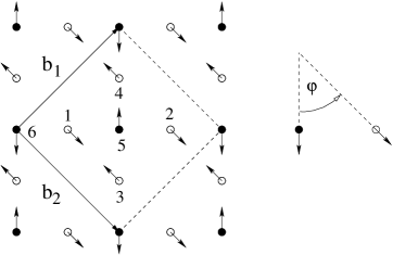
FIG. 2.: The classical ground state for $J_{AB}<2\sqrt{J_{AA}J_{BB}}$ (Néel phase I, cf. table I). Both subsystems possess Néel order. Because of the vanishing classical mean field both subsystems decouple magnetically and can freely rotate with respect to each other. The angle $\varphi$ is parametrizing this degree of freedom. The magnetic unit cell containing six spins is given by ${\bf{b}}_{1\left(2\right)}={\bf{a}}_{1}\pm{\bf{a}}_{2}$. The spins within the unit cell are labeled by a running index $n=1,\ldots,6$ corresponding to the six different magnons to be introduced in spin-wave theory.

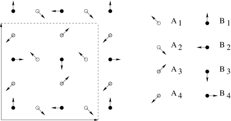
FIG. 3.: The spin orientations of phases II, III and IV. In the non-planar phase II there is an out-of-plane z component of the A spins illustrated by open and dashed circles, where the open circles and the dashed circles belong to opposite directions of the z component. In the planar phase III this out-of-plane z component is zero. In the non-planar phase IV the out-of-plane z component of A spins as well as of the B spins is uniform but opposite to each other. The magnetic unit cell of the magnetic states of phases II,III,IV contains twelve spins.

FIG. 4.: The finite A-B lattice with ${\cal N}=3N=24$ spins (periodic boundary conditions). The large circles (sites 1, …, 16) belong to subsystem A and the small circles to (sites 17, …, 24) to subsystem B.

FIG. 5.: A-A spin correlation $\langle{\bf S}^{A}_{i}{\bf S}^{A}_{j}\rangle$ for $(i,j)=(1,2)$ and $(i,j)=(1,7)$ (see Fig. 4) for the classical (thin lines, length of classical spin vectors is choosen as $s=1/2$) and the quantum (thick lines) model (${\cal N}=24$, $J_{AA}=1$, $J_{BB}=0.1$).

FIG. 6.: B-B spin correlation $\langle{\bf S}^{B}_{i}{\bf S}^{B}_{j}\rangle$ for $(i,j)=(17,24)$ and $(i,j)=(17,19)$ (see Fig. 4) for the classical (thin lines, length of classical spin vectors is choosen as $s=1/2$) and the quantum (thick lines) model (${\cal N}=24$, $J_{AA}=1$, $J_{BB}=0.1$).

FIG. 7.: A-B spin correlation $\langle{\bf S}^{A}_{i}{\bf S}^{B}_{j}\rangle$ for $(i,j)=(1,17)$ and $(i,j)=(1,24)$ (see Fig. 4) for the classical (thin lines, length of classical spin vectors is choosen as $s=1/2$) and the quantum (thick lines) model (${\cal N}=24$, $J_{AA}=1$, $J_{BB}=0.1$).

FIG. 8.: Scalar chirality $W$ (see eq. (15)) for the classical (solid line, length of classical spin vectors is choosen as $s=1/2$) and the quantum (crosses) model (${\cal N}=24$, $J_{AA}=1$, $J_{BB}=0.1$).

FIG. 9.: Ground-state energy per spin for $s=1/2$: spin-wave (${\cal N}=\infty$ and ${\cal N}=24$) and exact-diagonalization results and (${\cal N}=24$).

FIG. 10.: Sublattice magnetizations $\langle S_{A}^{z}\rangle$ and $\langle S_{B}^{z}\rangle$ (see eq. (32)) for $s=1/2$ in the infinite system: spin-wave results ($J_{AA}=1$, $J_{BB}=0.1$).

FIG. 11.: Nearest-neighbour correlation within the A subsystem and the B subsystem (exact diagonalization results for ${\cal N}=24$, $J_{AA}=1$, $J_{BB}=0.1$). For better comparison we have scaled $\langle{\bf S}_{i}{\bf S}_{j}\rangle$ by its corresponding values for $J_{AB}=0$.

REFERENCES

• [1] S.Noro, H.Suzuki, T. Yamadaya, Solid State Commun. 76, 711 (1990); S.Noro et al., Mater.Sci.Eng. B 25 (1994), 167.
• [2] K. Yamada, N. Suzuki, J. Akimitsu, Physica B 213-214, 191 (1995).
• [3] F.C. Chou et al., Phys. Rev. Lett. 78, 535 (1997).
• [4] Y.J. Kim et al., Phys. Rev. B 64, 024435 (2001).
• [5] A.B. Harris et al., Phys. Rev B 64, 024436 (2001).
• [6] T.V.Valyanskaya and V.I.Sokolov, Zh. Eksp. Teor. Fiz. 75, 325 (1978) (Sov. Phys. JETP 48, 161 (1978)).
• [7] E.F. Shender, Zh. Eksp. Teor. Fiz. 83, 326 (1982) (Sov. Phys. JETP 56, 178 (1982)).
• [8] Th.Brückel, C.Paulsen, K.Hinrichs and W.Prandl, Z.Phys. B 97, 391 (1995).
• [9] H.Rosner, R.Hayn and J.Schulenburg, Phys. Rev B 57, 13660 (1998).
• [10] J. Richter, A.Voigt, J.Schulenburg, N.B. Ivanov and R.Hayn, J. Magn. Magn. Mater. 177-181, 737 (1998).
• [11] N.B.Ivanov, J.Richter and D.J.J.Farnell, Phys. Rev B 66, 014421 (2002).
• [12] J. Villain, R. Bidaux, J.P. Carton, R. Conte, J. Phys. 41, 1263 (1980).
• [13] S.Krüger and J.Richter, Phys. Rev. B 64, 024433 (2001).
• [14] E.Dagotto and A.Moreo, Phys. Rev. Lett. 63, 2148 (1989).
• [15] H.J. Schulz and T.A.L. Ziman, Europhys. Lett. 18, 355 (1992).
• [16] J. Richter, Phys. Rev. B $\bf 47$, 5794 (1993).
• [17] L. Capriotti and S. Sorella, Phys. Rev. Lett. 84, 3173 (2000).
• [18] O.P. Sushkov, J. Oitmaa and Zheng Weihong, Phys. Rev. B 63, 104420 (2001).
• [19] R.P. Feynman, Phys. Rev. 56, 340 (1939).