Wave nucleation rate in excitable systems in the low noise limit

Abstract

Motivated by recent experiments on intracellular calcium dynamics, we study the general issue of fluctuation-induced nucleation of waves in excitable media. We utilize a stochastic Fitzhugh-Nagumo model for this study, a spatially-extended non-potential pair of equations driven by thermal (i.e. white) noise. The nucleation rate is determined by finding the most probable escape path via minimization of an action related to the deviation of the fields from their deterministic trajectories. Our results pave the way both for studies of more realistic models of calcium dynamics as well as of nucleation phenomena in other non-equilibrium pattern-forming processes.

One very important class of non-equilibrium spatially-extended systems is that of excitable media. In these, a quiescent state is linearly stable but nonlinear waves can nonetheless propagate without decaying. These waves can be generated by above-threshold local perturbations and they also can become self-sustaining in the form of rotating spiralsWinfree (1972). Examples of excitable media include many biological systems such as the cAMP waves seen in Dictyostelium amoebae aggregationLoomis (1975), electrical waves in cardiac and neural tissueWinfree (1987) and, primary for our focus here, intracellular calcium wavesBerridge et al. (2000).

Most excitable systems are sufficiently macroscopic as to render unimportant the role of thermodynamic fluctuations and allow for a description in terms of deterministic pde models. For these cases, noise effects can still be studied via the imposition of external variation in time and/or space (e.g. by varying illumination in a light-sensitive BZ reaction Sendi a-Nadal et al. (2001); Jung et al. (1998)); however, there is no need to include noise in a description of the “natural” version of these systems.

Figure 1: Left: Phase space diagram of the Fitzhugh-Nagumo system without noise and without the diffusive term. The stable equilibrium point is $O$. The $f(u,v)=3u-u^{3}-v$ nullcline is the S shaped solid line with minimum at $M$ and the $g=u+(1+\gamma)$ nullcline is the thin solid line. A small perturbation of $O$ leads to a large excursion in phase space. The dashed line shows the phase-space excursion of a point during the propagation of a single wave. Parameter values are $\gamma=.5$ and $\epsilon=0.05$. Right: Typical propagating wave in an excitable medium. Solid line: $u$; dashed line: $v$. The widths of the wave front and wave back (regions of fast change in $u$ where $(u,\,v)$ is not on the $f$ nullcline) are of order $\sqrt{\epsilon}$. The full return to equilibrium is not shown.

This is manifestly not the case for intracellular calcium dynamics; since the excitability here arises through the opening and closing of a small number of ion channels (allowing/preventing calcium efflux from calcium storesShuai and Jung (2002)), fluctuations are inherently non-negligible. Indeed, experiments show direct evidence of noise effects in the form of abortive waves and spontaneous wave nucleationLlano et al. (2000); Marchant et al. (1999).

In this paper, we study the process of spontaneous wave nucleation for a 1d generic excitable system modeled by the Fitzhugh-Nagumo equations

$$\partial_{t}u = (3u-u^{3}-v)/\epsilon+\nabla^{2}u+\eta_{u}$$ (1)

$$\partial_{t}v = u+(1+\gamma)+\eta_{v}$$ (2)

Here $\eta_{v}$ and $\eta_{u}$ are small independent white noise terms modeling fluctuation effects with covariance equal to:

$$<\eta_{i}(x,t)\eta_{j}(x^{\prime},t^{\prime})>=\beta\delta_{ij}\delta(x-x^{\prime})\delta(t-t^{\prime})$$ (3)

At $\beta=0$ and for positive values of $\gamma$, this system is excitable with a single stable equilibrium point $u_{0}=-(1+\gamma),\ v_{0}=3u_{0}-u_{0}^{3}$. As already mentioned, a wave of excitation can propagate through the system (see fig.1); a counter-propagating pair of such waves will be generated if a local perturbation above a threshold value is applied. For negative values of $\gamma$, the system becomes oscillatory. This model is not meant to be a realistic approximation for any specific physical or biological process; instead we use the model to understand the generic features of wave nucleation due to noise.

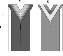
Figure 2: Space time contour plot of the $u$ (right) and $v$(left) field during nucleation with $T$=20; parameter values are $\epsilon=0.1$ and $\gamma=.2$. Time increases upward and the white area corresponds to the region outside of $[x_{min}(t)=max(x_{f}(t)-x_{off},0),x_{max}(t)=max(L+x_{f}(t)-x_{off},0)],\ [0,T]$. The contours are at -2, -1, 0, and 1 for the $u$ field and at $v_{0}-0.2$, $v_{0}-0.05$, $v_{0}+0.05$, $v_{0}+1$, $v_{0}+2$ and $v_{0}+3$ for the $v$ field. The lighter the surface, the higher the values of the fields are; thus, the light region of the $u$ contour plot corresponds to the excited region. After the nucleation event, points near the center reach the maximum of the excited branch of the $f$ nullcline (see fig. 1), return to the quiescent state and thereby give birth to the two wave-backs.

(a)	(b)
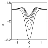
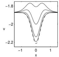
(c)	(d)

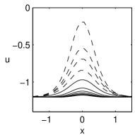
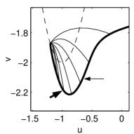
Figure 3: (a) and (b) $v$ profiles during a typical nucleation event. (a) $v$ profiles at times 25, 25.5, 26, 26.5, 27, 27.5 and 28. During that stage, the minimal value of the $v$ field decreases. (b) $v$ profiles at times 28(dashed), 28.25, 28.5, 28.75 and 29 (solid lines). During this stage, the minimal value of $v$ increases. (c): u profiles at the same times. The profiles corresponding to the (a),(b) curves are represented with a solid, dashed line. (d): The dashed line represents the $f$ nullcline. The thick solid line is the trajectory in the phase plane ($u(x=0,t),v(x=0,t)$) of the center of nucleation. The point where maximum value of $\int dx\delta_{u}^{2}+\delta_{v}^{2}$ is reached is indicated by a thick arrow, whereas the point where this deviation is below 1% of this maximal value is indicated by the thin arrow. Beyond this point the dynamics are mainly driven by the deterministic equations. The thin solid lines represent spatial snapshots of the MPEP ($u(x,t=T_{i}),\ v(x,t=T_{i})$) profile at regularly spaced points in time ($T_{i}-T_{i-1}=0.5$).

Specifically, at finite $\beta$ the noise will allow the birth of pairs of counter-propagating wave at a rate that will depend on the amplitude of the noise. That rate can be determined in the case of relatively high noise using direct numerical simulations. However, in the case of low noise, such a method becomes computationally prohibitive. Here we present a computation of the transition rate using a most probable escape path (MPEP) approach that is based on solving the Fokker-Planck equation Kramers (1940); Freidlin and Wentzell (1984). This method has been successfully applied to dynamical systemsGraham and Tél (1985); Maier and Stein (1993) and to a few cases of spatially extended systems, namely the transition from creep to fractureMarder (1995) and magnetic domain reversalWeinan et al. . To derive the equation for the MPEP, we use the fact that the solution of the Fokker-Planck equation with given initial and final field configurations for time interval $[0,T]$ can be written in terms of the path integral

$$P(T)=\int\mathcal{D}(u,v)\exp\left(-\frac{1}{\beta}\int\int\,dtdx\ S(x,t)\right)\\$$ (4)

with the “action density” $S$ given by the sum of the squared deviations of the time derivatives of the fields from their deterministic values: $S\equiv\delta_{u}^{2}+\delta_{v}^{2}$

$$\delta_{u} = \partial_{t}u-(3u-u^{3}-v)/\epsilon-\Delta u$$ (5)

$$\delta_{v} = \partial_{t}v-u-(1+\gamma)$$ (6)

The functional integral is taken over all paths that begin at $t=0$ in equilibrium and end with a given final counter-propagating wave state $(u_{f},v_{f})$ at $t=T$. Since we take $\beta$ close to 0, the r.h.s. of eq. (4) is dominated by the path (called most probable escape path or MPEP) that maximizes the integrand over all paths; thus, the transition rate is found to be proportional to:

$$\exp(-E/\beta)$$ (7)

where E is the minimum over all paths of $\int dx\int dt\,S$

Therefore, in order to compute the transition rate between the rest state and a pair of counter propagating waves, one has only to compute the minimum of the quantity in eq. (4). This minimum can be expressed using a variational principle as the solution of a PDEMarder (1996); however, using that approach to finding the actual MPEP between two different states involves the use of a shooting method with numerous parameters, which turns out to be numerically quite difficult. Instead, we used an alternative method based on discretizing the above path integral on a space-time grid and directly using a quasi-NewtonNocedal (1980) method to find the minimum. One difficulty with this approach is that the Fitzhugh Nagumo model has a slow recovery time compared to the timescale associated with a pulse (width of pulse/speed). This then necessitates having a very large spatial domain, if one attempts to completely encompass the region over which the nucleated wave configuration differs from the quiescent fixed point. To get around this difficulty, we use a grid moving with the pulse. That is, the grid moves in the same direction as the pulse in order to keep the wave front at a fixed distance from the boundary. Thus, the boundaries of the domain used to compute the MPEP path are no longer $[0,\,L],\,[0,T]$, but $[x_{min}(t)=0+\mbox{max}(x_{f}(t)-x_{off},0),\ x_{max}(t)=L+\mbox{max}(x_{f}(t)-x_{off},0)],\,[0,T]$, where $x_{f}(t)$ is the position of the wave front defined as the point where $u$ goes above 0 and $x_{off}$ is an arbitrary value lower than $L$ and significantly bigger than the wave front width. The following boundary conditions are applied:

$$\left\{\begin{array}[]{l}\mbox{at $x=x_{max}(t)$: }u=u_{0},\,v=v_{0}\\ \mbox{at $x=x_{min}(t)$: }\left\{\begin{array}[]{lcl}\partial_{x}u(0)=0&\mbox{ if }&x_{min}(t)=0\\ \delta_{u}(0)=0&\mbox{ if }&x_{min}(t)\neq 0\end{array}\right.\end{array}\right.$$ (8)

The condition $\delta_{u}=0$ implies that the recovery past $x_{min}$ is purely deterministic and hence does not contribute to $E$. A check on our procedure is afforded by the fact that as long as the distance the wave had traveled (in the final state) is significantly bigger than the region over which the wave initiates, the results obtained are independent both of the distance the wave had traveled and of the width of the space window used ($L$). We fix $T$ to be large enough that the deviation from deterministic dynamics for very small time is negligible. Once $T$ is fixed and the specific final wave state chosen, there is no time-translation invariance in the MPEP.

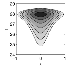
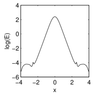
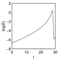
Figure 4: Parameters values are $\epsilon=0.1$ and $\gamma=.2$. Space time contour plot of the action density $\delta_{u}^{2}+\delta_{v}^{2}$ with its maximal value normalized to one. The contours are at $1/96,\ 1/48,\ 1/24,\ 1/12,\ 1/6,\ 1/3\mbox{ and }1/1.5$. (b) Left: spatial distribution of the contribution to $\log_{10}(E)$ during the MPEP; Right: temporal distribution of the contribution to $\log_{10}(E)$ during the MPEP. One can see that the contribution to $E$ as a function of time increases exponentially and then decreases rapidly to a very low level that is close to numerical noise

We now describe the results obtained using this methodology. In the small $\epsilon$ limit ($\epsilon<0.1$), the shape of the MPEP is quantitatively independent of $\epsilon$ and $\gamma$ and even for high values of $\epsilon$, there is no significant qualitative difference. In fig. 2, we present such a typical escape path. As shown on the contour plots, wave nucleation is found to be a very localized event. Essentially, the noise acts to create a local dip in value of the $v$ field which is then followed by a large positive excursion for the $u$ field as it goes into the excited phase. To describe this mechanism more fully, we present in fig. 3 the phase-plane trajectory at the center of nucleation as well as several snapshots of the spatial form of the fields during the nucleation process. One can see then that the escape path consists of the center of nucleation being driven by noise below the minimum of the $f$ nullcline; this then quickly drives the $u$ field positive and leads after, $v$-field driven relaxation, to the pair of counter-propagating pulses. There is a significant fluctuation contribution to the nucleation event in a small region around the nucleation point(see fig. 4). Results using different values of $\gamma$ and $\epsilon$ show that the width of that small region is proportional to the width of a front, that is $\sqrt{\epsilon}$ (see fig. 5). Note that the other simple possibility, that of nucleating an excited region for the $u$ field at a fixed value of $v$Pumir (1995), is not observed.

In accord with the shape of the trajectory, our calculations show that the main contribution to $E$ during the MPEP come from the $\int\int\delta_{v}^{2}$, at least for small values of $\epsilon$. Thus for $\gamma=0.2$ the value of the ratio $\int\int\delta_{v}^{2}/\int\int\delta_{u}^{2}$ never went below 30 for $\epsilon=0.1$, and went up to 1000 for the minimal value of $\epsilon$ used ($\epsilon=0.001$). For higher values of $\epsilon$, the ratio was significantly lower (3 for $\epsilon=0.8$, close to the limit of propagation for this value of $\gamma$ ). Furthermore for small $\epsilon$, $E$ scales like $\sqrt{\epsilon}$ (see fig. 5). For higher values of $\epsilon$, this simple scaling is no longer valid. The fact that for small values of $\epsilon$, $E$ scales like $\sqrt{\epsilon}$ and that a wave is therefore much easier to nucleate can be explained by a simple argument.

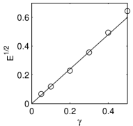
Figure 5: Left: circles $\log_{10}\epsilon$ dependence of $\log_{10}E$ using a log scale, solid line: $y=\frac{x}{2}-0.8$. For small $\epsilon$, $E$ behaves like $\sqrt{\epsilon}$. Right: circles $\gamma$ dependence of $\sqrt{E}$ for $\epsilon=0.1$. Solid, $y=1.2\,x$ $E$ behaves like $\gamma^{2}$ for a wide range of values of $\gamma$. The scaling breaks down for higher values of $\gamma$, close to the propagation threshold (for this value of $\epsilon$, the threshold is at $\gamma=0.5525\pm 0.0005$).

As already mentioned, the phase-plane trajectory of the MPEP is mainly independent of the value of $\epsilon$. The only dependence is then due to the spatial scale appearing in the integral which is $\sqrt{\epsilon}$, giving rise to the observed result

We now describe results obtained when varying $\gamma$ with $\epsilon$ held constant. This means that we consider the nucleation rates for differing excitabilities but with the same time-scale ratio between the $u$ and $v$ field dynamics. For a wide range of values of $\gamma$, we find that $E$ scaled like $\gamma^{2}$ (see fig. 5). The more excitable the system, the more likely it is to nucleate a wave. This scaling is that same as one would obtain analytically in the much simpler zero-dimensional version of this problem. Here the analog of wave nucleation is the noise-induced creation of a large transient excursion away from the fixed point. If $\epsilon$ is small, the escape path will follow the $f$ nullcline down to its minimum and then follow the noiseless dynamics to reach the other stable branch. In such a situation, one can compute the transition rate analytically in a piece-wise linear version of the FH model,

$$\dot{u} = \left\{\begin{array}[]{ll}-\frac{1}{\epsilon}(v+u)&\mbox{if $u<0$},\\ \frac{1}{\epsilon}(1-v-u)&\mbox{if $u\geq 0$},\end{array}\right.$$ (11)

$$\dot{v} = u-\gamma.$$ (12)

After elimination of $u$, it can easily be shown that the variational equation for the MPEP has the form

$$\frac{d^{2}v}{dt^{2}}=v+\gamma$$ (13)

with $v(0)=v_{0}=-\gamma$ and $v(T)=0$. A straightforward calculation shows that the action is equal to

$$\gamma^{2}\frac{1}{2(1-\exp(-2T))^{2}}$$ (14)

and that its minimum, reached for $T=\infty$, is equal to $\gamma^{2}/2$. This result shows that the $\gamma^{2}$ scaling of $E$ found in our computations can be interpreted as being due to $\gamma$ equaling the “distance” of the stable equilibrium point from the border of its basin of attraction. Putting it all together, our data yield a log transition rate proportional to $-\frac{\gamma^{2}\sqrt{\epsilon}}{\beta}$. This result could be tested experimentally, perhaps by adding illumination noise to the light-sensitive BZ reaction.

It is worth mentioning that there are other potential applications of the MPEP approach to nucleation in spatially-extended non-equilibrium systems. One example concerns the thermal generations of localized patches of traveling rolls in electro-convection, as studied recentlyBisang and Ahlers (1998). Also, the method used here is not limited to white noise. A simple generalization of the derivation allows for the incorporation of multiplicative noise via dividing the $\delta_{u}^{2}$ and $\delta_{v}^{2}$ terms in the action density by the corresponding (possibly field dependent) variances of the noises added to the $u$ and $v$ equations respectively. This will clearly be necessary for the study of realistic calcium models. Finally, there is a similarity between the MPEP method and what must be done to consider quantum tunneling in spatially extended systemsFreire et al. (1997), where one also must find the entire space-time path tunneling trajectory in order to find a leading estimate of the rate.

It is a pleasure to acknowledge useful discussions with D. Kessler. This research is supported by the National Science Foundation through Grant No. DMR-0101793.

References

- Winfree (1972) A. Winfree, Science 175, 634 (1972).
- Loomis (1975) W. F. Loomis, Dictyostelium discoideum, a developmental system (Academic Press New York, 1975).
- Winfree (1987) A. T. Winfree, When time breaks down (Princeton University Press, 1987).
- Berridge et al. (2000) M. Berridge, P. Lipp, and M. Bootman, Nature Reviews Molecular Cell Biology 1, 11 (2000).
- Sendi a-Nadal et al. (2001) I. Sendi a-Nadal, E. Mihaliuk, J. Wang, V. P rez-Mu uzuri, and K. Showalter, Physical Review Letters 86, 1646 (2001).
- Jung et al. (1998) P. Jung, A. cornell Bell, F. Moss, S. Kadar, J. Wang, and K. Showalter, Chaos 8, 567 (1998).
- Shuai and Jung (2002) J. Shuai and P. Jung, Biophysical Journal 83, 87 (2002).
- Llano et al. (2000) I. Llano, J. Gonz lez, C. Caputo, F. Lai, L. Blayney, Y. Tan, and A. Marty, Nature Neuroscience 3, 1256 (2000).
- Marchant et al. (1999) J. Marchant, N. Callamaras, and I. Parker, EMBO Journal 18, 5285 (1999).
- Kramers (1940) H. A. Kramers, Physica 7, 284 (1940).
- Freidlin and Wentzell (1984) M. Freidlin and A. Wentzell, Random perturbations of dynamical systems (Springer, New York, 1984).
- Graham and Tél (1985) R. Graham and T. Tél, Physical Review A 31, 1109 (1985).
- Maier and Stein (1993) R. Maier and D. Stein, Physical Review E 48, 931 (1993).
- Marder (1995) M. Marder, Physical Review Letters 74, 4547 (1995).
- (15) E. Weinan, R. Weiqing, and E. Vanden-Eijnden, Cond-Mat/0205168 April 2002.
- Marder (1996) M. Marder, Physical Review E 54, 3442 (1996).
- Nocedal (1980) J. Nocedal, Mathematics of Computation 35, 773 (1980).
- Pumir (1995) A. Pumir, Journal de Physique II 5, 1533 (1995).
- Bisang and Ahlers (1998) U. Bisang and G. Ahlers, Physical Review Letters 80, 3061 (1998).
- Freire et al. (1997) J. Freire, D. Arovas, and H. Levine, Physical Review Letters 79, 5054 (1997).