Abstract

It is believed that strong ferromagnetic orders in some solids are generated by subtle interplay between quantum many-body effects and spin-independent Coulomb interactions between electrons. Here we describe our rigorous and constructive approach to ferromagnetism in the Hubbard model, which is a standard idealized model for strongly interacting electrons in a solid. We introduce a class of Hubbard models in any dimensions which are nonsingular in the sense that both the Coulomb interaction and the density of states (at the Fermi level) are finite. We then prove that the ground states of the models exhibit saturated ferromagnetism, i.e., have maximum total spins. Combined with our earlier results, the present work provides nonsingular models of itinerant electrons with only spin-independent interactions where low energy behaviors are proved to be that of a “healthy” ferromagnetic insulator.

1 Introduction

The origin of strong ferromagnetic order observed in some solids has long been a mystery in physical science. After Heisenberg [1], it became clear that the ultimate origin of ferromagnetism lies in a subtle interplay between quantum many-body effects and strong Coulomb interaction between electrons. To provide convincing derivations of ferromagnetism in concrete models of many electrons, however, remained unsolved (even on a heuristic level) for a long time.

The problem is difficult because neither quantum many-body effects, nor the Coulomb interaction alone favors ferromagnetism (or any magnetic ordering). One must deal with an interplay of both the factors. Moreover, the intrinsically nonperturbative nature of the phenomenon makes the problem almost impossible to attack within conventional perturbative methods in condensed matter physics. A generic many-electron system without interactions is known to have a paramagnetic ground state, a phenomenon known as Pauli paramagnetism. In order to destabilize Pauli paramagnetism and stabilize ferromagnetism, one must have a sufficiently large interaction. For example, a heuristic argument due to Stoner implies the criterion that $U\,D_{\rm F}\mathrel{\raisebox{-2.8pt}{\mbox{$\stackrel{{\scriptstyle\textstyle>}}{{\sim}}$}}}1$ is necessary to stabilize ferromagnetism, where $U$ is the on-site Coulomb interaction and $D_{\rm F}$ is the density of states at the Fermi level. This is the well-known “competition” between quantum dynamics and Coulomb interaction.

In the present paper, we describe our constructive and mathematically rigorous approach to the origin of ferromagnetism. This is a continuation of the series of works [2, 3, 4, 5], and the main result of the present paper was described in [6] for a special one-dimensional model. Here we present a class of Hubbard models in any dimensions with a finite density of states (at the Fermi level) and finite interactions, and prove that their ground states are ferromagnetic. Combined with our earlier work [4, 5], this provides a class of nonsingular models of itinerant electrons (with only spin-independent interactions) in which low energy behaviors (i.e., the nature of the ground states and the low-lying excitations) are rigorously proved to be those expected in ferromagnetic insulators. We hope that the present work becomes a starting point of further investigations of deep interplay between quantum dynamics and nonlinear interactions in strongly interacting quantum many-body systems.

The present paper is written in a nearly self-contained manner. In Section 2, we give the definition of the Hubbard model. In Section 3, we briefly review rigorous results about ferromagnetism in the Hubbard model, and motivate the present paper. In Section 4, we summarize, in a typical class of models, the main results of our constructive program in the present and the previous works of ours. The reader who is interested in the new physical results is invited to start from this section. In Section 5, which is the main section of the paper, we define our models in the most general setting and state our conclusions precisely. Final section 6 is devoted to the proof of the main theorem.

2 Definition of the Hubbard model

The Hubbard model is a standard simple model of interacting itinerant electrons in a solid. Although this model is too idealized to be regarded as a quantitatively reliable model of real solids, it contains physically essential features of interacting itinerant electron systems. It is expected to exhibit various phenomena including antiferromagnetism, ferromagnetism, ferrimagnetism, superconductivity, and metal-insulator transition. Some (but not all) of these phenomena have been treated rigorously in some cases [7].

In the present section, we define the Hubbard model in the general setting, and fix our notation. We leave details and backgrounds to more careful reviews (such as [7, 8, 9]) and present only the minimum necessary ingredients.

2.1 Basic operators

Let a lattice $\Lambda$ be a finite set whose elements $r,s,\cdots\in\Lambda$ are called sites. A site represents an atomic orbit in a solid.

For each $r\in\Lambda$ and $\sigma=\uparrow,\downarrow$, we define the creation and the annihilation operators $c^{\dagger}_{r,\sigma}$ and $c_{r,\sigma}$ for an electron at site $r$ with spin $\sigma$. These operators satisfy the canonical anticommutation relations

$$\{c^{\dagger}_{r,\sigma},c_{s,\tau}\}=\delta_{r,s}\,\delta_{\sigma,\tau},$$ (2.1)

and

$$\{c^{\dagger}_{r,\sigma},c^{\dagger}_{s,\tau}\}=\{c_{r,\sigma},c_{s,\tau}\}=0,$$ (2.2)

for any $r,s\in\Lambda$ and $\sigma,\tau=\uparrow,\downarrow$, where $\{A,B\}=AB+BA$. The number operator is defined by

$$n_{r,\sigma}=c^{\dagger}_{r,\sigma}\,c_{r,\sigma},$$ (2.3)

which has eigenvalues 0 and 1.

The Hilbert space of the model is constructed as follows. Let $\Phi_{\rm vac}$ be a normalized vector state which satisfies $c_{r,\sigma}\Phi_{\rm vac}=0$ for any $r\in\Lambda$ and $\sigma=\uparrow,\downarrow$. Physically $\Phi_{\rm vac}$ corresponds to a state where there are no electrons in the system. Then for arbitrary subsets $\Lambda_{\uparrow},\Lambda_{\downarrow}\subset\Lambda$, we define a state

$$\left(\prod_{r\in\Lambda_{\uparrow}}c^{\dagger}_{r,\uparrow}\right)\left(\prod_{r\in\Lambda_{\downarrow}}c^{\dagger}_{r,\downarrow}\right)\Phi_{\rm vac},$$ (2.4)

in which sites in $\Lambda_{\uparrow}$ are occupied by up-spin electrons and sites in $\Lambda_{\downarrow}$ by down-spin electrons. The Hilbert space for the system with $N_{\rm e}$ electrons is spanned by the basis states (2.4) with all subsets $\Lambda_{\uparrow}$ and $\Lambda_{\downarrow}$ such that $|\Lambda_{\uparrow}|+|\Lambda_{\downarrow}|=N_{\rm e}$.

We finally define total spin operators $\hat{\bf S}_{\rm tot}=(\hat{S}^{(1)}_{\rm tot},\hat{S}^{(2)}_{\rm tot},\hat{S}^{(3)}_{\rm tot})$ by

$$\hat{S}^{(\alpha)}_{\rm tot}=\frac{1}{2}\mathop{\sum_{r\in\Lambda}}_{\sigma,\tau=\uparrow,\downarrow}c^{\dagger}_{r,\sigma}(p^{(\alpha)})_{\sigma,\tau}\,c_{r,\tau},$$ (2.5)

for $\alpha=1$, 2, and 3. Here $p^{(\alpha)}$ are the Pauli matrices defined by

$$p^{(1)}=\pmatrix{0&1\cr 1&0\cr},\quad p^{(2)}=\pmatrix{0&-i\cr i&0\cr},\quad p^{(3)}=\pmatrix{1&0\cr 0&-1\cr}.$$ (2.6)

The operators $\hat{\bf S}_{\rm tot}$ are the generators of $SU(2)$ rotations of the total spin angular momentum of the system. As usual we denote the eigenvalue of $(\hat{\bf S}_{\rm tot})^{2}$ as $S_{\rm tot}(S_{\rm tot}+1)$. The maximum possible value of $S_{\rm tot}$ is $N_{\rm e}/2$ when $N_{\rm e}\leq|\Lambda|$.

2.2 General Hamiltonian

The model is characterized by the hopping amplitudes $t_{r,s}=t_{s,r}\in\mathbb{R}$ defined for all $r,s\in\Lambda$, and the magnitude $U>0$ of the on-site Coulomb interaction. Physically, $t_{r,s}$ represents the quantum mechanical amplitude for an electron to hop from the site $s$ to site $r$ when $s\neq r$, and the on-site potential when $r=s$. Usually $t_{r,s}$ is non-negligible only when the two sites $r$ and $s$ are close to each other.

We then define the general Hubbard Hamiltonian as

$$H=\mathop{\sum_{r,s\in\Lambda}}_{\sigma=\uparrow,\downarrow}t_{r,s}\,c^{\dagger}_{r,\sigma}c_{s,\sigma}+U\sum_{r\in\Lambda}n_{r,\uparrow}n_{r,\downarrow}.$$ (2.7)

Here the first term describes quantum mechanical motion of electrons which hop around the lattice according to the amplitude $t_{r,s}$.

The second term represents nonlinear interactions between electrons. There is an increase in energy by $U>0$ for each doubly occupied site, i.e., a site which is occupied by both up-spin electron and down-spin electron. This is a highly idealized treatment of the Coulomb interaction between electrons.

The Hamiltonian which consists only of the first term in (2.7) describes the free tight-binding electron model. It is not very difficult to analyze this model especially when the hopping amplitude $t_{r,s}$ has a translation invariance. The Hamiltonian can be diagonalized in the states in which electrons behave as “waves.”

The Hamiltonian which consists only of the second term in (2.7) is also easy to study. The Hamiltonian is already diagonalized in the basis states (2.4), in which electrons behave as “particles.”

When both the first and the second terms in (2.7) are present, a “competition” between wave-like nature and particle-like nature of electrons takes place. The competition generates rich nontrivial phenomena including ferromagnetism. To investigate these phenomena is a main motivation in the study of the Hubbard model.

3 Rigorous results about ferromagnetism in the Hubbard model

In the present section, we formulate the problem of saturated ferromagnetism in the Hubbard model. We then give a brief review of the rigorous results about ferromagnetism in the Hubbard model, and explain background of the present work. For more careful reviews, see [8, 9].

3.1 Saturated ferromagnetism in the ground states

It is easily shown that the Hamiltonian (2.7) commutes with the total spin operators $\hat{S}^{(\alpha)}_{\rm tot}$. Therefore one can look for simultaneous eigenstates of $H$ and $(\hat{\bf S}_{\rm tot})^{2}$.

When all the ground states of the Hamiltonian $H$ (with a fixed electron number $N_{\rm e}\leq|\Lambda|$) are eigenstate of $(\hat{\bf S}_{\rm tot})^{2}$ with $S_{\rm tot}=N_{\rm e}/2$, we say that the model exhibits saturated ferromagnetism. This is the strongest form of ferromagnetism since $N_{\rm e}/2$ is the maximum possible value for $S_{\rm tot}$.

3.2 Ferromagnetism of Nagaoka and Thouless

The first rigorous and nontrivial result about saturated ferromagnetism in the Hubbard model is due to Nagaoka [10] and to Thouless [11]. It was proved that the Hubbard model on a class of lattices (which includes most of the standard lattices in two and three dimensions) with $t_{r,s}\geq 0$ exhibits saturated ferromagnetism when $N_{\rm e}=|\Lambda|-1$ and $U=\infty$. In other words the model is not allowed to have any doubly occupied sites, and there is only one site without an electron.

The ferromagnetism of Nagaoka and Thouless is quite important since it showed for the first time that the Hubbard model can generate ferromagnetism through nontrivial interplay between quantum dynamics and Coulomb interaction. Subsequent studies, however, have suggested that their mechanism of ferromagnetism is restricted to special situation with infinite $U$ and a single hole. See Section 4 of [8] for a modern proof and further discussions.

3.3 Lieb’s ferrimagnetism and flat-band ferromagnetism

In 1989, after more than two decades from the works of Nagaoka and Thouless, Lieb proved an important theorem for the Hubbard model with $N_{\rm e}=|\Lambda|$ (i.e., half-filling) on a bipartite lattice [12]. For the Hubbard model with $U>0$ on lattices which have two sublattices with different numbers of sites, Lieb’s theorem implies the existence of ferrimagnetism, a weaker version of ferromagnetism. A typical example is the Hubbard model on the so called copper oxide lattice of Fig. 1, where the ground states are proved to have $S_{\rm tot}=N_{\rm e}/6$ when $N_{\rm e}=|\Lambda|$. The models exhibiting Lieb’s ferrimagnetism have peculiar single-electron band structures where the band at the middle of the spectrum is completely flat (or dispersionless). One may regard Lieb’s ferrimagnetism as a precursor to the flat-band ferromagnetism that we shall discuss.

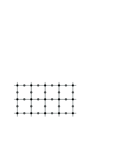
Figure 1: The so called copper oxide lattice. As a consequence of Lieb’s theorem [12], it is proved that the Hubbard model with $U>0$ on this lattice has $S_{\rm tot}=N_{\rm e}/6$ when $N_{\rm e}=|\Lambda|$.

Flat-band ferromagnetism was discovered first by Mielke [13, 14, 15] and then by Tasaki [2, 3]. Mielke treated the Hubbard model on a general line graph, where $t_{r,s}=t>0$ for those pairs $(r,s)$ corresponding to the edges (or bonds) of the lattice, and $t_{r,s}=0$ otherwise. The models have peculiar band structure where the lowest single-electron band is completely flat. Mielke proved that the models with $U>0$ exhibit saturated ferromagnetism for suitable electron numbers which correspond to the half-filling of the lowest bands. A typical example (and the most beautiful example of flat-band ferromagnetism) is the Hubbard model on the kagomé lattice of Fig.2, which was proved to exhibit saturated ferromagnetism when $N_{\rm e}=|\Lambda|/3$. See also [16, 17, 18] for Mielke’s results on Hubbard models with partially flat bands.

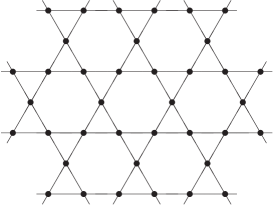
Figure 2: The kagomé lattice is the line graph of the hexagonal lattice. Mielke [13, 14, 15] showed that the Hubbard model on the kagomé lattice exhibits ferromagnetism when $N_{\rm e}=|\Lambda|/3$ for any $U>0$.

Tasaki [2, 3] proposed his version of Hubbard models with flat lowest bands, and proved the existence of saturated ferromagnetism for $U>0$ when the lowest bands are half-filled. As can be seen from the one-dimensional example in Fig. 3, his models have two different kinds of lattice sites which are sometimes interpreted as metallic and oxide atoms, and have next nearest neighbor hopping amplitudes. By fine-tuning the hopping amplitudes and the on-site potentials, the lowest band becomes flat. See [19] for an extension.

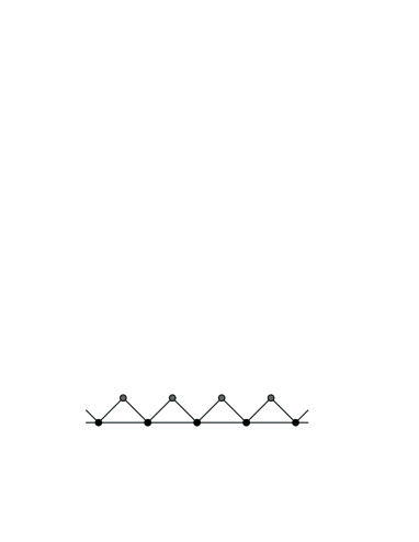
Figure 3: Tasaki’s flat-band Hubbard model in one dimension [2, 3]. The hopping amplitude $t_{r,s}$ is $\nu^{2}t$ for the horizontal bonds and $\nu t$ for the diagonal bonds. The sites in the upper and the lower rows have on-site potential $t_{r,r}$ which equal $t$ and $2\nu^{2}t$, respectively. When $N_{\rm e}=|\Lambda|/2$, the model exhibits saturated ferromagnetism for any $t>0$, $\nu>0$, and $U>0$. See Theorem 4.1.

A common feature of Lieb’s ferrimagnetism and Mielke’s and Tasaki’s ferromagnetism is that their models have single-electron bands which are totally flat (i.e., dispersionless), and the magnetization is supported by electrons in the flat bands. (For Lieb’s ferrimagnetism, the latter statement is correct only in a vague sense.) This observation is consistent with the Stoner criterion which states that large $UD_{\rm F}$ favors ferromagnetism. Here the criterion is realized by infinitely large density of states $D_{\rm F}$.

The works of Lieb, Mielke, and Tasaki have shown that rich classes of Hubbard models on slightly complicated lattices exhibit nontrivial magnetic behavior. Such a view may be helpful in understanding insulating ferromagnetism observed in a cuprate [20, 8], and has even motivated some scientists to design novel ferromagnetic materials. See [21] and references therein. But one should not forget that the Hubbard model is a highly idealized model. To find implications of the results for the Hubbard model in realistic many-electron systems defined in continuum space is a formidably difficult but a challenging problem. See, for example, [21, 22].

3.4 Beyond flat-band ferromagnetism

Although Lieb’s ferrimagnetism and Mielke’s and Tasaki’s flat-band ferromagnetism certainly have shed novel light on the mechanisms of magnetic ordering in interacting electron systems, they do not deal with the true “competition” between quantum dynamics and Coulomb interactions. When the Coulomb interaction $U$ is vanishing, all of their models have highly degenerate ground states. The degeneracy reflects the existence of completely flat bands. Among these degenerate ground states for $U=0$, there are ferrimagnetic or ferromagnetic states as well as states with much smaller magnetization. The role of the Coulomb interaction in these models is simply to lift the huge degeneracy and “select” the states with highest magnetization as unique ground states. Consequently ferrimagnetism or ferromagnetism in these models takes place for any values of $U>0$. In other words magnetic ordering is stabilized by infinitesimally small Coulomb interaction. This is quite different from situations in realistic systems where the interaction must be greater than some positive critical value in order to destabilize Pauli paramagnetism and get magnetic ordering.

It may be needless to say that the existence of completely flat lowest bands (especially in Tasaki’s models) is unrealistic, or even pathological. The flatness of the bands is destroyed by arbitrarily small generic perturbation, and is far from robust.

It was therefore highly desirable to go beyond flat band models. A natural step was to modify the model by adding extra hopping terms to the Hamiltonian thus making the flat band dispersive, and then to show that the magnetic ordering survives. One can only hope this scenario to work for sufficiently large $U$ since magnetic ordering becomes truly a nonperturbative phenomenon when the band is not flat.

As the first step in this direction, the local stability of the ferromagnetic state was proved in models obtained by adding arbitrary small short-range hopping terms to Tasaki’s version of flat-band Hubbard models [4, 5]. In this work, it was also shown that low-lying excitation energy above the ferromagnetic state has the dispersion relation expected for a magnon excitation. Then it was proved in [6] that a one-dimensional Hubbard model with non-flat bands exhibits saturated ferromagnetism for sufficiently large $U$. The model was obtained by adding extra nearest neighbor hopping terms to Tasaki’s one-dimensional flat-band Hubbard model as in Fig. 4. This was the first rigorous example of ferromagnetism in an electron system without any singularities, i.e., with finite interaction and finite density of states. Shen [23] announced a computer assisted extension of the proof in [6] to some higher dimensional models. The method in [6] inspired similar rigorous works in different classes of Hubbard models [24, 25]. In particular Tanaka and Ueda [26] recently succeeded in proving the existence of saturated ferromagnetism in a Hubbard model obtained by adding extra hopping terms to Mielke’s flat band Hubbard model on the kagomé lattice. For closely related heuristic works, see [27, 28] and other references in Section 6.6 of [8].

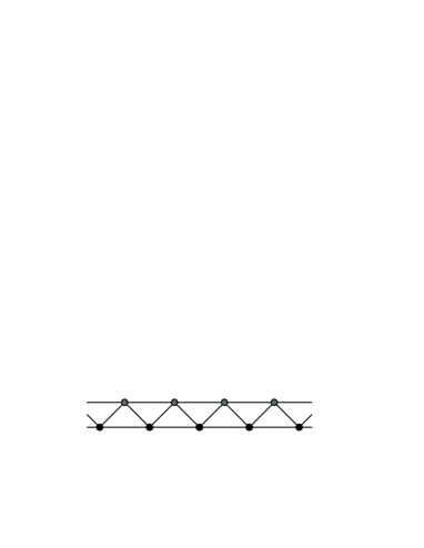
Figure 4: Tasaki’s nearly-flat-band Hubbard model in one dimension [6]. The hopping amplitude $t_{r,s}$ is $-\nu^{2}s$ and $\nu^{2}t$ for the horizontal bonds in the upper and the lower rows, respectively, and $\nu(t+s)$ for the diagonal bonds. The sites in the upper and the lower row have on-site potential $t_{r,r}$ which equal $t-2\nu^{2}s$ and $2\nu^{2}t-s$, respectively. The model has two bands which are not flat. When $N_{\rm e}=|\Lambda|/2$, the model exhibits saturated ferromagnetism for sufficiently large $U/s$ and $t/s$ for any $\nu>0$. When $\nu=1/\sqrt{2}$, for example, the appearance of ferromagnetism is proved for $t/s\geq 1.6$ and sufficiently large $U/s$. See Theorem 4.2.

The present work is an extension of that in [6]. We extend the theorem in [6] to general models in higher dimensions. As was noted in [6], a straightforward extension of the method in [6] applies to a class of higher dimensional models. Instead of using such a method, we here present a much more general and simplified proof which naturally covers a more general class of models.

4 Ferromagnetism in typical $d$-dimensional nearly-flat-band models

In the present section, we concentrate on a simple class of models defined on decorated hypercubic lattices, and precisely describe the results of the present paper and our previous works. Although our works cover much more general models, it may be useful for the readers to see what has been achieved in the context of simple models. In short, we start from a concretely defined non-singular model of itinerant electrons, and prove that its low energy properties coincide with what one expects in a “healthy” ferromagnet.

Let ${\cal E}$ denote (only in the present section) the $d$-dimensional $L\times\cdots\times L$ hypercubic lattice with the unit lattice spacing and periodic boundary conditions. We let $L>0$ to be an odd integer. We take a new site in the middle of each bond (i.e., a pair of neighboring sites) in ${\cal E}$, and denote by ${\cal I}$ (again only in this section) the collection of all such sites. We shall study the decorated hypercubic lattice $\Lambda={\cal E}\cup{\cal I}$ in the present section. See Fig. 5.

We define a Hubbard model on $\Lambda$ which is characterized by four parameters $t>0$, $s>0$, $\nu>0$, and $U>0$. The hopping amplitude of the model is given by

$$t_{r,s}=\cases{\nu(t+s)&if $|r-s|=1/2$;\cr\nu^{2}t&if $r,s\in{\cal E}$ and $|r-s|=1$;\cr-\nu^{2}s&if $(r,s)\in{\cal B}$;\cr 2d\nu^{2}t-s&if $r=s\in{\cal E}$;\cr t-2\nu^{2}s&if $r=s\in{\cal I}$;\cr 0&otherwise,}$$ (4.1)

where we set

$${\cal B}=\left\{(r,s)\,\Bigl{|}\,r,s\in{\cal I},\ |r-s|=1/\sqrt{2}\right\}\cup\left\{(r,s)\,\Bigl{|}\,r,s\in{\cal I},\ |r-s|=1,\ (r+s)/2\in{\cal E}\right\}.$$ (4.2)

There are nearest neighbor and next nearest neighbor hopping amplitudes. See Fig. 5. This rather complicated expression for $t_{r,s}$ comes from a simple construction in Section 5.3. See (5.12).

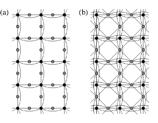
Figure 5: The lattice structure and the hopping amplitudes in the two dimensional model. The black dots are sites in ${\cal E}$, and the gray dots are sites in ${\cal I}$. (a) shows the flat-band model with $s=0$, and (b) shows general model with $s>0$.

One can easily calculate the single-electron properties corresponding to the above hopping amplitudes. There are $(d+1)$ single-electron bands and their dispersion relations are given by

$$\varepsilon_{j}(k)=\cases{-s-2\nu^{2}s\sum_{\mu=1}^{d}(1+\cos k_{\mu})&if $j=1$;\cr t&if $j=2,\cdots,d$;\cr t+2\nu^{2}t\sum_{\mu=1}^{d}(1+\cos k_{\mu})&if $j=d+1$.}$$ (4.3)

Here $k=(k_{1},\ldots,k_{d})$ is the wave vector in the set

$${\cal K}=\left\{(\frac{2\pi}{L}n_{1},\ldots,\frac{2\pi}{L}n_{d})\,\Bigl{|}\,n_{i}=0,\pm 1,\pm 2,\ldots,\pm\frac{L-1}{2}\right\}.$$ (4.4)

In the flat-band model with $s=0$, all the bands except the uppermost band with $j=d+1$ are dispersionless (or flat) as in Fig. 6 (a). In a general model with $s>0$, the lowest band becomes dispersive as in Fig. 6 (b). Since our ferromagnetism is supported by electrons in the lowest band, it is crucial that the lowest band becomes dispersive. Reflecting the special geometry of the decorated lattice, the intermediate bands with $j=2,\ldots,d$ are always dispersionless. This, however, is not crucial to low energy behavior of our model. Indeed it is not difficult to add proper extra hopping terms to the model to make all the bands dispersive while maintaining the existence of ferromagnetism. See Section 6.2.

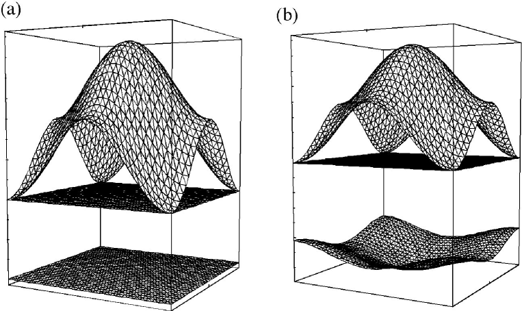
Figure 6: The dispersion relation (4.3) of the single-electron bands in the two dimensional model. The horizontal axes represent $-\pi\leq k_{1},k_{2}\leq\pi$, and the vertical axis denotes the single-electron energy. (a) shows the flat-band model with $s=0$, and (b) shows general model with $s>0$.

We consider the Hubbard model with the Hamiltonian (2.7), the hopping amplitudes (4.1), and the electron number $N_{\rm e}=|{\cal E}|=L^{d}$.

We first recall the result about the flat-band ferromagnetism proved in [2, 3]. (See Section 6 of [8] for the most compact proof.)

Theorem 4.1 (Flat-band ferromagnetism)

Let $s=0$. Then for arbitrary $t>0$, $\nu>0$, and $U>0$, the above model exhibits saturated ferromagnetism.

As we have stressed in Section 3.4, ferromagnetism takes place for any positive values of $U$ in the flat-band models. When the lowest band is no longer flat, saturated ferromagnetism cannot take place for too small values of $U>0$. This fact can be seen, for example, from the following (easy and well-known) theorem. (See Section 3.3 of [8] for a proof.)

Theorem 4.2 (Instability of saturated ferromagnetism)

Let $s>0$ and $U<4\nu^{2}s$. Then the lowest energy among the states with $S_{\rm tot}=S_{\rm max}-1$ is strictly lower than the lowest energy among the states with $S_{\rm tot}=S_{\rm max}$. This means that the ground state of the model has $S_{\rm tot}<S_{\rm max}$, and hence the model does not exhibit saturated ferromagnetism.

The theorem, unfortunately, does not tell us what the ground states look like for small $U$. (We nevertheless believe that the model has ground states with $S_{\rm tot}=0$ for sufficiently small $U$.) It assures us, however, that the appearance of saturated ferromagnetism, which is established in the following theorem, is a purely nonperturbative phenomenon.

Theorem 4.3 (Ferromagnetism in nearly-flat-band models)

When $t/s$, $U/s$, and $1/\nu$ are sufficiently large (how large these quantities should be depend only on the dimensionality $d$), the above model exhibits saturated ferromagnetism.

This is a special case of our main theorem in the present paper, Theorem 5.2. For the model with $d=1$, one can prove the same statement for any values of $\nu>0$. See Section 6.2. A computer assisted proof of the above theorem for $d=2,3$ (which makes use of an extension of the method in [6]) was announced by Shen [23].

Moreover our earlier results in [4, 5] about low-lying excitations also apply to the present model. For any $x\in{\mathbb{Z}}^{d}$, define the translation operator $T_{x}$ by

$$T_{x}\left[\left(\prod_{r\in\Lambda_{\uparrow}}c^{\dagger}_{r,\uparrow}\right)\left(\prod_{r\in\Lambda_{\downarrow}}c^{\dagger}_{r,\downarrow}\right)\Phi_{\rm vac}\right]=\left(\prod_{r\in\Lambda_{\uparrow}}c^{\dagger}_{r+x,\uparrow}\right)\left(\prod_{r\in\Lambda_{\downarrow}}c^{\dagger}_{r+x,\downarrow}\right)\Phi_{\rm vac},$$ (4.5)

where we use periodic boundary conditions to identify $r+x$ with a site in $\Lambda$ (if necessary). Then, for any $k\in{\cal K}$, we let $E_{\rm SW}(k)$ be the lowest possible energy among the states that satisfy $\hat{S}_{\rm tot}^{(3)}\Phi=\{(N_{\rm e}/2)-1\}\Phi$ and $T_{x}[\Phi]=e^{ik\cdot x}\Phi$ for any $x$. In other words, $E_{\rm SW}(k)$ is the lowest energy among the states where a single spin is flipped (from the ferromagnetic ground state) and the total momentum is $k$. Then we have the following theorem. (For more precise statements, see Section 3.3 of [5].)

Theorem 4.4 (Dispersion relation of low-lying excitations)

Let $E_{\rm GS}$ be the ground state energy. When $t/s$, $U/s$, $t/U$, and $1/\nu$ are sufficiently large, one has

$$F_{1}\,{4\nu^{4}U}\sum_{\mu=1}^{d}(\sin\frac{k_{\mu}}{2})^{2}\geq E_{\rm SW}(k)-E_{\rm GS}\geq F_{2}\,{4\nu^{4}U}\sum_{\mu=1}^{d}(\sin\frac{k_{\mu}}{2})^{2},$$ (4.6)

for any $k\in{\cal K}$. Moreover the constants $F_{1}$ and $F_{2}$ tend to 1 as $s\to 0$ and $\nu\to 0$.

Therefore, for sufficiently small $s$ and $\nu$, we have an almost precise estimate

$$E_{\rm SW}(k)-E_{\rm GS}\simeq{4\nu^{4}U}\sum_{\mu=1}^{d}(\sin\frac{k_{\mu}}{2})^{2},$$ (4.7)

about the low-lying excitation energies. We note that this dispersion relation is what one expects for the elementary magnon excitation in a ferromagnetic Heisenberg model on ${\cal E}$ with the exchange interaction $J_{\rm eff}=2\nu^{4}U$.

To summarize, we have obtained a class of non-singular models of itinerant electrons (with only spin-independent interactions) whose low energy behaviors are rigorously proved to be that of a “healthy” insulating ferromagnet. By a “healthy” insulator, we mean an itinerant electron system whose low energy properties can effectively be described by an appropriate quantum spin systems. Although we can hardly claim that our model is realistic, the similarity with ferromagnetism observed in a cuprate (see Section 7.1 of [8]) suggests that our models share some features with some of the existing ferromagnetic insulators.

Let us finally discuss whether our ferromagnetism is robust against perturbations. We note that Theorem 4.4 about the low-lying excitation is still valid when one adds small arbitrary translation invariant perturbation to the hopping amplitudes. In other words, local stability of the ferromagnetic state is proved for slightly perturbed models. Since it is generally believed that local stability of ferromagnetism implies global stability (see [17] for a related rigorous result), this strongly suggests that the global stability of ferromagnetism (as is stated in Theorem 4.3) is valid for general perturbed models.

5 The model and main results

5.1 Construction of the lattice

We define our lattice and the Hubbard model on it.

Let us give a brief explanation first. Our lattice $\Lambda$ consists of two kinds of sites called external sites and internal sites. The sets of all the external and the internal sites are denoted as ${\cal E}$ and ${\cal I}$, respectively. In the model of Fig. 5, for example, the black dots are external sites and gray dots are internal sites. The whole lattice $\Lambda$ is decomposed into a union of overlapping cells. Each cell contains a single internal site and $n$ ($n\geq 2$) external sites. An internal site $u$ belongs to exactly one cell (denoted as $C_{u}$), while an external site $x$ belongs to $m$ ($m\geq 2$) cells. In Fig. 5, a bond which consists of two black dots and a gray dot is a cell.

To be more precise, let us define the general lattice by using the “cell construction” as in [8]. This allows us to cover a general class of models in a unified manner.

We fix two integers $n,m\geq 2$ which will characterize our lattice. Let the basic cell be a set of $(n+1)$ sites written as

$$C=\{u,x_{1},x_{2},\cdots,x_{n}\}.$$ (5.1)

For convenience, we call $u$ the internal site of $C$, and $x_{1},x_{2},\cdots,x_{n}$ the external sites.

To form the lattice $\Lambda$, we assemble $M$ identical copies of the basic cell, and identify external sites from $m$ distinct cells regarding them as a single site. We do not make such identifications for internal sites. We assume that the lattice $\Lambda$ thus constructed is connected. Usually $\Lambda$ becomes a periodic lattice by this construction.

The lattice $\Lambda$ is naturally decomposed as

$$\Lambda={\cal I}\cup{\cal E},$$ (5.2)

where ${\cal I}$ and ${\cal E}$ are the sets of internal sites and external sites, respectively. From the above construction, we see that the numbers of sites in these sublattices are $|{\cal I}|=M$ and $|{\cal E}|=nM/m$.

See Figure 7 for some examples of the basic cell and corresponding lattices. The examples treated in Section 4 are obtained by considering the cell with $n=2$, and setting $m=2d$.

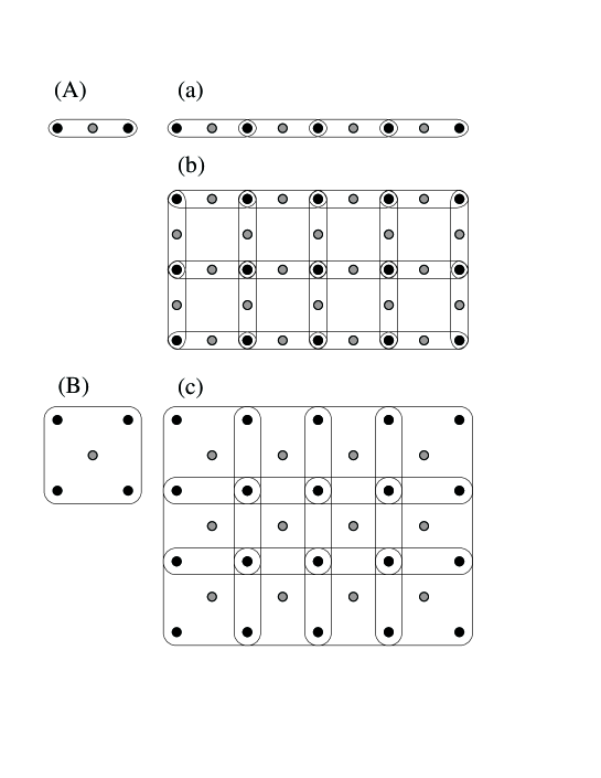
Figure 7: Examples of cells and lattices. The black dots represent external sites, and the gray dots represent internal sites. (A) From the cell with three sites ($n=2$), one can form (a) a one-dimensional lattice (which is drawn as the delta chain or the zigzag chain in Figs. 3 and 4) by identifying two external sites ($m=2$), or (b) a decorated square lattice (which also appears in Fig. 5) by identifying four ($m=4$). (B) From the cell with five sites ($n=4$), one can form, for example, (c) another decorated square lattice (which will appear in Fig. 8) by identifying four external sites ($m=4$). There are many similar examples in higher dimensions.

We can easily treat models where $n$ and $m$ are not identical for different cells, but we here concentrate on the simplest case with constant $n$ and $m$. (We still can treat a variety of lattices by choosing different $n$, $m$, and ways of assembling the cells.)

For an internal site $u\in{\cal I}$, we denote by $C_{u}\subset\Lambda$ the cell which contains the site $u$. For an external site $x\in{\cal E}$, we denote by $\Lambda_{x}\subset\Lambda$ the union of $m$ cells which contain the site $x$.

5.2 Fermion operators

We define special fermion operators which will be crucial for our analysis. Let $\nu>0$ be a constant. (We note that $1/\nu$ corresponds to $\lambda$ in our previous publications [2, 3, 4, 5, 8].) For $x\in{\cal E}$, let

$$a_{x,\sigma}=c_{x,\sigma}-\nu\sum_{u\in\Lambda_{x}\cap{\cal I}}c_{u,\sigma},$$ (5.3)

where the sum is over $m$ internal sites adjacent to $x$. Similarly for $u\in{\cal I}$, let

$$b_{u,\sigma}=c_{u,\sigma}+\nu\sum_{x\in C_{u}\backslash\{u\}}c_{x,\sigma},$$ (5.4)

where the sum is over the $n$ external sites adjacent to $u$.

From the anticommutation relations (2.1) for the basic $c$ operators, one can easily verify that

$$\{a^{\dagger}_{x,\sigma},b_{u,\tau}\}=0$$ (5.5)

for any $x\in{\cal E}$, $u\in{\cal I}$, and $\sigma,\tau=\uparrow,\downarrow$. This means that the $a$ operators and the $b$ operators correspond to distinct spaces of electrons. We shall discuss more about this point in Section 5.4.

The anticommutation relations between the $a$ operators are

$$\{a^{\dagger}_{x,\sigma},a_{y,\tau}\}=\cases{1+m\nu^{2},&if $x=y$, $\sigma=\tau$;\cr\ell_{x,y}\,\nu^{2},&if $x\neq y$, $\sigma=\tau$;\cr 0,&if $\sigma\neq\tau$.}$$ (5.6)

For $x,y\in{\cal E}$, we defined

$$\ell_{x,y}=|\Lambda_{x}\cap\Lambda_{y}\cap{\cal I}|,$$ (5.7)

which is the number of distinct cells which contain both $x$ and $y$. For the $b$ operators, we similarly have

$$\{b^{\dagger}_{u,\sigma},b_{v,\tau}\}=\cases{1+n\nu^{2},&if $u=v$, $\sigma=\tau$;\cr\ell_{u,v}\,\nu^{2},&if $u\neq v$, $\sigma=\tau$;\cr 0,&if $\sigma\neq\tau$.}$$ (5.8)

For $u,v\in{\cal I}$, we defined

$$\ell_{u,v}=|C_{u}\cap C_{v}\cap{\cal E}|,$$ (5.9)

which is the number of external sites which are adjacent to both $u$ and $v$. One sees that $a$ operators or $b$ operators simply anticommute with each other if the reference sites are sufficiently separated. The slightly complicated anticommutation relations (found for sufficiently close reference sites) reflect the use of basis states which are localized but not orthogonal with each other.

An important property of the $a$ and $b$ operators is that one can represent arbitrary states of the system by using these operators. The key is the following lemma.

Lemma 5.1

For any $r\in\Lambda$ and $\sigma=\uparrow,\downarrow$, one has

$$c_{r,\sigma}=\sum_{x\in{\cal E}}\gamma_{x}\,a_{x,\sigma}+\sum_{u\in{\cal I}}\eta_{u}\,b_{u,\sigma},$$ (5.10)

with suitable coefficients $\gamma_{x}$ and $\eta_{u}$.

Proof: Consider a Hilbert space which consists of operators of the form $\sum_{r\in\Lambda}\alpha_{r}\,c_{r,\sigma}$ with $\alpha_{r}\in\mathbb{C}$. We fix $\sigma$ to be either $\uparrow$ or $\downarrow$. The inner product of the two “vectors” $\sum_{r\in\Lambda}\alpha_{r}\,c_{r,\sigma}$ and $\sum_{r\in\Lambda}\beta_{r}\,c_{r,\sigma}$ is defined to be the anticommutator $\{(\sum_{r\in\Lambda}\alpha_{r}\,c_{r,\sigma})^{\dagger},\sum_{r\in\Lambda}\beta_{r}\,c_{r,\sigma}\}=\sum_{r\in\Lambda}\overline{\alpha_{r}}\,\beta_{r}$. Since $\{a^{\dagger}_{x,\sigma},b_{u,\sigma}\}=0$ for any $x\in{\cal E}$ and any $u\in{\cal I}$, the subspace spanned by the set $\{a_{x,\sigma}\}_{x\in{\cal E}}$ and that spanned by the set $\{b_{u,\sigma}\}_{u\in{\cal I}}$ are orthogonal. Since $a_{x,\sigma}$ with different $x$ are linearly independent, the dimension of the former subspace is equal to $|{\cal E}|$. Similarly the dimension of the latter subspace is $|{\cal I}|$. Noting that $|{\cal E}|+|{\cal I}|=|\Lambda|$ is the dimension of the whole space, one finds that the set $\{a_{x,\sigma}\}_{x\in{\cal E}}\cup\{b_{u,\sigma}\}_{u\in{\cal I}}$ spans the whole space. This means that any $c_{r,\sigma}$ can be expanded in terms of $a_{x,\sigma}$ and $b_{u,\sigma}$ as in (5.10).  

Recall that the basis states of the many-electron Hilbert space are (2.4). As a consequence of the lemma, we find that an arbitrary many-electron state of the system can be represented as a linear combination of the basis states

$$\Psi_{0}^{(\nu)}(E_{\uparrow},E_{\downarrow},I_{\uparrow},I_{\downarrow})=\left(\prod_{x\in E_{\uparrow}}a^{\dagger}_{x,\uparrow}\right)\left(\prod_{x\in E_{\downarrow}}a^{\dagger}_{x,\downarrow}\right)\left(\prod_{u\in I_{\uparrow}}b^{\dagger}_{u,\uparrow}\right)\left(\prod_{u\in I_{\downarrow}}b^{\dagger}_{u,\downarrow}\right)\Phi_{\rm vac},$$ (5.11)

with arbitrary subsets $E_{\uparrow},E_{\downarrow}\subset{\cal E}$ and $I_{\uparrow},I_{\downarrow}\subset{\cal I}$. Here $|E_{\uparrow}|+|E_{\downarrow}|+|I_{\uparrow}|+|I_{\downarrow}|=N_{\rm e}$ is the total electron number.

5.3 Definition of the model and the main theorem

Our model is characterized by the four parameters $t>0$, $s>0$, $U>0$, and $\nu>0$. The Hamiltonian of the model on $\Lambda$ is

$$H=-s\mathop{\sum_{x\in{\cal E}}}_{\sigma=\uparrow,\downarrow}a^{\dagger}_{x,\sigma}\,a_{x,\sigma}+t\mathop{\sum_{u\in{\cal I}}}_{\sigma=\uparrow,\downarrow}b^{\dagger}_{u,\sigma}\,b_{u,\sigma}+U\sum_{r\in\Lambda}n_{r,\uparrow}n_{r,\downarrow},$$ (5.12)

where the number operator $n_{x,\sigma}$ is defined in (2.3).

Recalling the definitions (5.3) and (5.4), one sees that this defines a Hubbard model with nearest and next nearest neighbor hopping terms. We can rewrite (5.12) in the standard form (2.7) with the hopping matrix given by

$$\cases{t_{x,x}=mt\nu^{2}-s,&$x\in{\cal E}$\cr t_{u,u}=t-ns\nu^{2},&$u\in{\cal I}$\cr t_{x,u}=t_{u,x}=\cases{\nu(t+s),&$x\in C_{u}$\cr 0,&$x\not\in C_{u}$\cr}&$x\in{\cal E}$, $u\in{\cal I}$\cr t_{x,y}=\ell_{x,y}\,\nu^{2}t,&$x,y\in{\cal E}$, $x\neq y$\cr t_{u,v}=-\ell_{u,v}\,\nu^{2}s,&$u,v\in{\cal I}$, $u\neq v$\cr}$$ (5.13)

Note that the model has nearest and next-nearest neighbor hopping amplitudes, but not more. See Figs. 4, 5 (b), and 8 for examples.

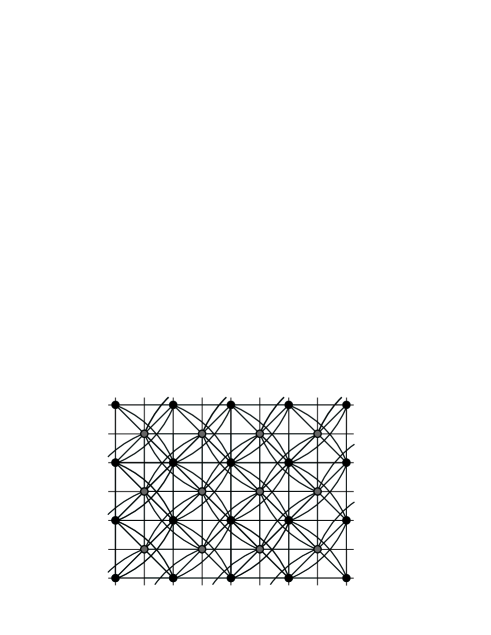
Figure 8: Another example on the fcc like lattice in two dimensions obtained by setting $n=m=4$.

We consider the Hilbert space with the electron number fixed to $N_{\rm e}=|{\cal E}|=nM/m$. Note that this electron number is consistent with the interpretation that an external site represents a metallic atom which emits one electron to the system.

Exactly as in Theorem 4.1, it can be shown that the flat-band models with $s=0$ exhibit saturated ferromagnetism for any $t>0$, $\nu>0$ and $U>0$. See Section 6 of [8] for a proof. The instability of saturated ferromagnetism for sufficiently small $U$ as in Theorem 4.2 can be of course proved for the general models. See Section 3.3 of [8].

Our main result is the following theorem which shows that the ground states of the model exhibit saturated ferromagnetism.

Theorem 5.2

When $t/s$, $U/s$ and $1/\nu$ are sufficiently large (how large these quantities should be depends only on the local structure of the lattice, but not on the size of the lattice), the ground state of the model is $(N_{\rm e}+1)$-fold degenerate and has the total spin $S_{\rm tot}=N_{\rm e}/2$.

In the proof of the theorem, we further show that one of the ground states is written as

$$\Phi_{\rm GS}=\left(\prod_{x\in{\cal E}}a^{\dagger}_{x,\uparrow}\right)\Phi_{\rm vac},$$ (5.14)

and other ground states are obtained by applying the spin lowering operator $\hat{S}^{-}_{\rm tot}=\sum_{r\in\Lambda}c^{\dagger}_{r,\downarrow}c_{r,\uparrow}$ onto the state (5.14).

5.4 “Band” structure in the single-electron problem

Before proceeding to prove the theorem, we discuss a basic property of the single electron problem associated with the present model. Although the discussion is not necessary for the proof of the main theorem, it sheds light on a special character of the model that we are studying.

The single electron Hilbert space $\mathfrak{h}$ is the $|\Lambda|$-dimensional linear space spanned by $c^{\dagger}_{r,\uparrow}\Phi_{\rm vac}$ with $r\in\Lambda$. (We here consider the space of up-spin electrons, but this choice is not essential.) This space is decomposed as

$$\mathfrak{h}=\mathfrak{h}_{\rm L}\oplus\mathfrak{h}_{\rm U},$$ (5.15)

where $\mathfrak{h}_{\rm L}$ is spanned by $a^{\dagger}_{x,\uparrow}\Phi_{\rm vac}$ with $x\in{\cal E}$, and $\mathfrak{h}_{\rm U}$ by $b^{\dagger}_{u,\uparrow}\Phi_{\rm vac}$ with $u\in{\cal I}$. Then we have the following.

Proposition 5.3

The Hamiltonian $H$ can be diagonalized within $\mathfrak{h}_{\rm L}$ and within $\mathfrak{h}_{\rm U}$, respectively. The energy eigenvalues $\epsilon$ in $\mathfrak{h}_{\rm L}$ satisfy

$$-s\{1+(m+\ell_{\rm L})\nu^{2}\}\leq\epsilon\leq\min\{0,-s\{1+(m-\ell_{\rm L})\nu^{2}\}\},$$ (5.16)

where $\ell_{\rm L}=\sum_{y\in{\cal E},y\not=x}\ell_{x,y}$ with $x\in{\cal E}$, and the energy eigenvalues $\epsilon$ in $\mathfrak{h}_{\rm U}$ satisfy

$$\max\{0,t\{1+(n-\ell_{\rm U})\nu^{2}\}\}\leq\epsilon\leq t\{1+(n+\ell_{\rm U})\nu^{2}\},$$ (5.17)

where $\ell_{\rm U}=\sum_{v\in{\cal I},v\not=u}\ell_{u,v}$ with $u\in{\cal I}$.

The proposition states that the spectrum of the Hamiltonian $H$ in the single electron Hilbert space $\mathfrak{h}$ consists of two distinct “bands.” When $\nu$ is sufficiently small (which is the case when the theorem holds), the two “bands” do not overlap and are separated by a finite gap. The fermion operator $a^{\dagger}_{x,\sigma}$ creates an electron in the lower “band”, and $b^{\dagger}_{u,\sigma}$ creates an electron in the upper “band.”

When the model has a translation invariance as in the models of Section 4, the single electron Hilbert space is decomposed into several bands in the standard sense. The lower or upper “band” that we mentioned above is not necessarily a band in the usual sense, but may be a union of several bands. In the band structure (4.3) discussed in Section 4, the lowest band with $j=1$ corresponds to the lower “band”, and the collection of the remaining $d$ bands corresponds to the upper “band.”

Proof: The proof is elementary but requires some care.

Consider a state $\Phi$ of the form

$$\Phi=\sum_{x\in{\cal E}}\varphi(x)a^{\dagger}_{x,\uparrow}\Phi_{\rm vac},$$ (5.18)

where $\varphi(x)$ are complex coefficients. From the anticommutation relations (5.6), one finds that

$$H\Phi=-\sum_{x\in{\cal E}}s\left\{(1+m\nu^{2})\varphi(x)+\nu^{2}\mathop{\sum_{y\in{\cal E}}}_{y\not=x}\ell_{x,y}\varphi(y)\right\}a^{\dagger}_{x,\uparrow}\Phi_{\rm vac}.$$ (5.19)

Since the right-hand side is again a linear combination of $a^{\dagger}_{x,\uparrow}\Phi_{\rm vac}$, we find that $H$ can be diagonalized within $\mathfrak{h}_{\rm L}$. We now assume $H\Phi=\epsilon\Phi$. By comparing the coefficients in (5.18) and (5.19), we find

$$-s(1+m\nu^{2})\varphi(x)-s\nu^{2}\mathop{\sum_{y\in{\cal E}}}_{y\not=x}\ell_{x,y}\varphi(y)=\epsilon\,\varphi(x).$$ (5.20)

By multiplying (5.20) with $\overline{\varphi(x)}$, by summing it over $x\in{\cal E}$, and by solving it for $\epsilon$, one gets

$$\epsilon=-\left(\sum_{x\in{\cal E}}|\varphi(x)|^{2}\right)^{-1}\left(s(1+m\nu^{2})\sum_{x\in{\cal E}}|\varphi(x)|^{2}+s\nu^{2}\mathop{\sum_{x,y\in{\cal E}}}_{x\not=y}\ell_{x,y}\,\overline{\varphi(x)}\,\varphi(y)\right).$$ (5.21)

By using the inequalities

$$-(|\varphi(x)|^{2}+|\varphi(y)|^{2})\leq\overline{\varphi(x)}\,\varphi(y)+\varphi(x)\,\overline{\varphi(y)}\leq|\varphi(x)|^{2}+|\varphi(y)|^{2},$$ (5.22)

which follow immediately from $|\varphi(x)\pm\varphi(y)|^{2}\geq 0$, we find from (5.21) that

$$-s(1+m\nu^{2})-s\nu^{2}\ell_{\rm L}\leq\epsilon\leq-s(1+m\nu^{2})+s\nu^{2}\ell_{\rm L}.$$ (5.23)

This, with the positive semidefiniteness of $a^{\dagger}_{x,\sigma}a_{x,\sigma}$, proves the desired (5.16). The other inequality (5.17) is proved in exactly the same manner using the $b^{\dagger}_{u,\uparrow}$ operators.  

6 Proof

6.1 Proof of the main theorem

The basic strategy of the proof is first to show the appearance of ferromagnetism in a local piece of the system, and then to “connect” these local ferromagnetism together to get the desired ferromagnetic state on the whole system. Of course such a “connection” usually does not work in itinerant electron systems where electrons behave as “waves.” Our method makes a full use of special features of our model as well as of ferromagnetic states.

Our proof is based on the decomposition of the Hamiltonian

$$H=\sum_{x\in{\cal E}}h_{x},$$ (6.1)

where $h_{x}$ acts only on the sublattice $\Lambda_{x}$. The local Hamiltonian $h_{x}$ is defined as

$$h_{x}=-s\sum_{\sigma=\uparrow,\downarrow}a^{\dagger}_{x,\sigma}a_{x,\sigma}+\frac{t}{n}\mathop{\sum_{u\in\Lambda_{x}\cap{\cal I}}}_{\sigma=\uparrow,\downarrow}b^{\dagger}_{u,\sigma}b_{u,\sigma}+\frac{U}{n^{\prime}}\sum_{y\in\Lambda_{x}\cap{\cal E}}n_{y,\uparrow}n_{y,\downarrow}+\frac{U}{n}\sum_{u\in\Lambda_{x}\cap{\cal I}}n_{u,\uparrow}n_{u,\downarrow},$$ (6.2)

where $n^{\prime}=|\Lambda_{x}\cap{\cal E}|$. It should be stressed that $h_{x}$ with neighboring $x$ do not commute with each other. One therefore cannot diagonalize all $h_{x}$ simultaneously.

As for the lowest eigenvalue and the corresponding eigenstates, however, we have the following. This lemma plays a key role in our proof of the theorem.

Lemma 6.1

When $t/s$, $U/s$ and $1/\nu$ are sufficiently large, the lowest eigenvalue of $h_{x}$ is $-s(1+m\nu^{2})$, and any corresponding eigenstate $\Phi$ can always be written as

$$\Phi=a^{\dagger}_{x,\uparrow}\Phi_{1}+a^{\dagger}_{x,\downarrow}\Phi_{2},$$ (6.3)

where $\Phi_{1}$, $\Phi_{2}$ are suitable states with $N_{\rm e}-1$ electrons. The eigenstate $\Phi$ also satisfies

$$c_{r,\uparrow}c_{r,\downarrow}\Phi=0,$$ (6.4)

for any $r\in\Lambda_{x}$.

We shall prove Theorem 5.2 assuming Lemma 6.1. The lemma will be proved in Section 6.3.

Since $h_{x}\geq-s(1+m\nu^{2})$, we have $H=\sum_{x\in{\cal E}}h_{x}\geq-s(1+m\nu^{2})|{\cal E}|$. A straightforward calculation using the anticommutation relations (5.5) and (5.6) shows that the state (5.14) is an eigenstate of $H$ with the eigenvalue $-s(1+m\nu^{2})|{\cal E}|$. Therefore we see that the state (5.14) is a ground state. Our goal here is to characterize all the ground states.

Let $\Phi$ be an arbitrary eigenstate of $H$ with the eigenvalue $-s(1+m\nu^{2})|{\cal E}|$. Then it follows from $h_{x}\geq-s(1+m\nu^{2})$ that

$$h_{x}\Phi=-s(1+m\nu^{2})\Phi,$$ (6.5)

for any $x\in{\cal E}$. Thus $\Phi$ satisfies the properties stated in Lemma 6.1.

Let us expand $\Phi$ in the basis states $\Psi_{0}^{(\nu)}(E_{\uparrow},E_{\downarrow},I_{\uparrow},I_{\downarrow})$ of (5.11). Since $\Phi$ satisfies (6.3) for any $x\in{\cal E}$, it follows that only those basis states with $E_{\uparrow}\cup E_{\downarrow}={\cal E}$ contribute. Since the electron number is $|E_{\uparrow}|+|E_{\downarrow}|+|I_{\uparrow}|+|I_{\downarrow}|=N_{\rm e}=|{\cal E}|$, the condition $E_{\uparrow}\cup E_{\downarrow}={\cal E}$ implies $E_{\uparrow}\cap E_{\downarrow}=\emptyset$ and $I_{\uparrow}=I_{\downarrow}=\emptyset$. Therefore the expansion of $\Phi$ in the basis states (5.11) can be rearranged into a “spin system representation” as

$$\Phi=\sum_{\boldsymbol{\sigma}}\psi(\boldsymbol{\sigma})\left(\prod_{x\in{\cal E}}a^{\dagger}_{x,\sigma(x)}\right)\Phi_{\rm vac},$$ (6.6)

where $\boldsymbol{\sigma}=(\sigma(x))_{x\in{\cal E}}$ is summed over all the spin configurations with $\sigma(x)=\uparrow,\downarrow$, and $\psi(\boldsymbol{\sigma})$ are complex coefficients.

We then examine the property (6.4) for $u\in{\cal I}$. From the definition (5.3), we find that for any $u\in{\cal I}$

$$c_{u,\uparrow}c_{u,\downarrow}\left(\prod_{x\in{\cal E}}a^{\dagger}_{x,\sigma(x)}\right)\Phi_{\rm vac}=\mathop{\sum_{y,z\in C_{u}\backslash\{u\}}}_{y\not=z}{\rm sgn}(y,z)\,\chi[\sigma(y)=\uparrow,\sigma(z)=\downarrow]\left(\prod_{x\in{\cal E}\backslash\{y,z\}}a^{\dagger}_{x,\sigma(x)}\right)\Phi_{\rm vac},$$ (6.7)

where the sign factor ${\rm sgn}(y,z)$ comes from the anticommutation relations, and satisfies ${\rm sgn}(y,z)=-{\rm sgn}(z,y)$. The characteristic function $\chi[\cdot]$ is defined as usual by $\chi[{\rm true}]=1$ and $\chi[{\rm false}]=0$. By using (6.6) and (6.7), we find for any $u\in{\cal I}$ that

$$c_{u,\uparrow}c_{u,\downarrow}\Phi=\mathop{\sum_{y,z\in C_{u}\backslash\{u\}}}_{y>z}\sum_{\boldsymbol{\sigma}}{\rm sgn}(y,z)\,\chi[\sigma(y)=\uparrow,\sigma(z)=\downarrow]\,\{\psi(\boldsymbol{\sigma})-\psi(\boldsymbol{\sigma}_{y\rightleftharpoons z})\}\left(\prod_{x\in{\cal E}\backslash\{y,z\}}a^{\dagger}_{x,\sigma(x)}\right)\Phi_{\rm vac},$$ (6.8)

where we have introduced an arbitrary ordering in ${\cal E}$ to avoid double counting. The spin configuration $\boldsymbol{\sigma}_{y\rightleftharpoons z}$ is obtained from $\boldsymbol{\sigma}=(\sigma(x))_{x\in{\cal E}}$ by switching $\sigma(y)$ and $\sigma(z)$. Since the basis states in the sum (6.8) are all linearly independent, we find from the property (6.4) that

$$\psi(\boldsymbol{\sigma})=\psi(\boldsymbol{\sigma}_{y\rightleftharpoons z}),$$ (6.9)

for any $y,z\in{\cal E}$ for which there is $u\in{\cal I}$ such that $y,z\in C_{u}$. Since the whole lattice is connected, (6.9) implies that all $\psi(\boldsymbol{\sigma})$ with the same $M=\sum_{x\in{\cal E}}\sigma(x)$ are identical. This completes the characterization of the space of the ground states. The ground state which has a fixed total spin in the $z$-direction is

$$\Phi_{M}=\mathop{\sum_{\boldsymbol{\sigma}}}_{\sum_{x}\sigma(x)=M}\left(\prod_{x\in{\cal E}}a^{\dagger}_{x,\sigma(x)}\right)\Phi_{\rm vac},$$ (6.10)

where $M=-(|{\cal E}|/2),1-(|{\cal E}|/2),,\cdots,(|{\cal E}|/2)-1,|{\cal E}|/2$. Thus the ground states are $|{\cal E}|+1$ fold degenerate. It is easy to check that

$$(\hat{\bf S}_{\rm tot})^{2}\Phi_{M}=S_{\rm max}(S_{\rm max}+1)\Phi_{M},\quad\hat{S}^{(z)}_{\rm tot}\Phi_{M}=M\,\Phi_{M},$$ (6.11)

with $S_{\rm max}=|{\cal E}|/2$ being the maximum possible value of the total spin of $N_{\rm e}=|{\cal E}|$ electrons.

6.2 Some extensions

Let us make two brief remarks about extensions of Theorem 5.2.

The first extension deals with the one dimensional model of Fig. 4, which (in the notation of Section 5.1) has $n=m=2$. In this model, Tanaka [29] observed that the statement of Theorem 5.2 can be proved if one first fixes arbitrary $\nu>0$ and then takes sufficiently large $t/s$ and $U/s$.

To show this extended theorem, one proves the statement corresponding to Lemma 6.1 by the method we used in [6] to prove the similar lemma. The differences between the lemma in [6] and that in the present paper comes from a difference in the definitions of the local Hamiltonian. Unlike the definition (6.2) in the present paper, we did not include the on-site repulsion terms from the external sites other than $x$ in the local Hamiltonian used in [6]. This seemingly minor difference indeed makes a considerable difference in the conditions that we obtain in the limit $U\to\infty$. The same method as in [6] thus yields much stronger information for the local Hamiltonian defined as in the present paper. We leave the details to the interested readers.

The second extension is much more straightforward and less important. For arbitrary complex coefficients $f_{u}$, define

$$B=\sum_{\sigma=\uparrow,\downarrow}\left\{\sum_{u\in{\cal I}}f_{u}b_{u,\sigma}\right\}^{\dagger}\left\{\sum_{u\in{\cal I}}f_{u}b_{u,\sigma}\right\},$$ (6.12)

which is obviously positive semidefinite. From the expression (6.11) for the ground states and the anticommutation relations (5.5), one readily finds that $B\Phi=0$ for any ground state $\Phi$.

This means that one may add to the Hamiltonian the new hopping terms

$$H^{\prime}=\sum_{j}\sum_{\sigma=\uparrow,\downarrow}\left\{\sum_{u\in{\cal I}}f_{u}^{(j)}b_{u,\sigma}\right\}^{\dagger}\left\{\sum_{u\in{\cal I}}f_{u}^{(j)}b_{u,\sigma}\right\},$$ (6.13)

with arbitrary $f^{(j)}_{u}$ without modifying the ferromagnetic ground states. In this manner, one can modify, for example, the models in Section 4 so that all the bands become dispersive maintaining the appearance (and the provability) of saturated ferromagnetism.

6.3 Proof of Lemma 6.1

It suffices to prove the lemma for $h_{o}$ with a fixed $o\in{\cal E}$. Since $h_{o}$ acts only on $\Lambda_{o}$, we only consider an electron system defined on $\Lambda_{o}$ without specifying the electron number. We also write ${\cal E}_{o}=\Lambda_{o}\cap{\cal E}$ and ${\cal I}_{o}=\Lambda_{o}\cap{\cal I}$. The local Hamiltonian that we consider is

$$h_{o}=-s\sum_{\sigma=\uparrow,\downarrow}a^{\dagger}_{o,\sigma}a_{o,\sigma}+\frac{t}{n}\mathop{\sum_{u\in{\cal I}_{o}}}_{\sigma=\uparrow,\downarrow}b^{\dagger}_{u,\sigma}b_{u,\sigma}+\frac{U}{n^{\prime}}\sum_{x\in{\cal E}_{o}}n_{x,\uparrow}n_{x,\downarrow}+\frac{U}{n}\sum_{u\in{\cal I}_{o}}n_{u,\uparrow}n_{u,\downarrow}.$$ (6.14)

We stress that the statement of the Lemma is about the property of a finite dimensional matrix $h_{o}$. It is thus possible (in principle) to prove the lemma for fixed $n$, $m$ by using a computer. But the problem is indeed rather delicate, and the proof for general cases seems highly nontrivial.

As we have restricted our lattice, we redefine (only in this proof) the operator $a_{x,\sigma}$ for $x\in{\cal E}_{o}\backslash\{o\}$ as

$$a_{x,\sigma}=c_{x,\sigma}-\nu\sum_{u\in\Lambda_{x}\cap{\cal I}_{o}}c_{u,\sigma}.$$ (6.15)

The definition of $b_{u,\sigma}$ is unchanged. Note that we still have $\{a^{\dagger}_{x,\sigma},b_{u,\tau}\}=0$.

Exactly as in (5.11), any state defined on $\Lambda_{o}$ can be written as a linear combination of the basis states

$$\Psi_{1}^{(\nu)}(E_{\uparrow},E_{\downarrow},I_{\uparrow},I_{\downarrow})=\left(\prod_{x\in E_{\uparrow}}a^{\dagger}_{x,\uparrow}\right)\left(\prod_{x\in E_{\downarrow}}a^{\dagger}_{x,\downarrow}\right)\left(\prod_{u\in I_{\uparrow}}b^{\dagger}_{u,\uparrow}\right)\left(\prod_{u\in I_{\downarrow}}b^{\dagger}_{u,\downarrow}\right)\Phi_{\rm vac},$$ (6.16)

with arbitrary subsets $E_{\uparrow},E_{\downarrow}\subset{\cal E}_{o}$ and $I_{\uparrow},I_{\downarrow}\subset{\cal I}_{o}$. Here we do not fix the electron number which is given by $|E_{\uparrow}|+|E_{\downarrow}|+|I_{\uparrow}|+|I_{\downarrow}|$.

6.3.1 The limit $t,U\to\infty$

Let us first consider the limit where $t\to\infty$ and $U\to\infty$. It is easily found that the lowest eigenvalue of $h_{o}$ is finite in this limit. (Try, for example, the state $a^{\dagger}_{o,\uparrow}\Phi_{\rm vac}$.) Note that the parts in $h_{o}$ which contain $t$ are $(t/n)\sum_{u\in{\cal I}_{o}}\sum_{\sigma=\uparrow,\downarrow}b^{\dagger}_{u,\sigma}b_{u,\sigma}$, and which contain $U$ are $(U/n^{\prime})\sum_{x\in{\cal E}_{o}}n_{x,\uparrow}n_{x,\downarrow}+(U/n)\sum_{u\in{\cal I}_{o}}n_{u,\uparrow}n_{u,\downarrow}$. Since each term in these sums is positive semidefinite, the necessary and sufficient condition for a state $\Phi$ to have a finite energy in the limit $t\to\infty$, $U\to\infty$ is

$$b_{u,\sigma}\Phi=0,$$ (6.17)

for any $u\in{\cal I}_{o}$ and $\sigma=\uparrow,\downarrow$, and

$$c_{r,\uparrow}c_{r,\downarrow}\Phi=0$$ (6.18)

for any $r\in\Lambda_{o}$. To get (6.18), we noted that $n_{r,\uparrow}n_{r,\downarrow}=(c_{r,\uparrow}c_{r,\downarrow})^{\dagger}c_{r,\uparrow}c_{r,\downarrow}$.

To see implications of the condition (6.17), we introduce dual operators $\tilde{b}_{u,\sigma}$ for $u\in{\cal I}_{o}$ and $\sigma=\uparrow,\downarrow$ which satisfy

$$\{\tilde{b}_{u,\sigma},b^{\dagger}_{v,\tau}\}=\delta_{u,v}\,\delta_{\sigma,\tau},$$ (6.19)

for any $u,v\in{\cal I}_{o}$ and $\sigma,\tau=\uparrow,\downarrow$. More precisely the construction is as follows. Define the Gramm matrix ${\sf G}$ by $({\sf G})_{u,v}=\{b_{u,\sigma},b^{\dagger}_{v,\sigma}\}$, where $u,v$ run over ${\cal I}_{o}$. The linear independence of the basis states implies that ${\sf G}$ is invertible. For $u\in{\cal I}_{o}$ and $\sigma=\uparrow,\downarrow$, define

$$\tilde{b}_{u,\sigma}=\sum_{w\in{\cal I}_{o}}({\sf G}^{-1})_{u,w}\,b_{w,\sigma},$$ (6.20)

where it is easy to check (6.19).

From (6.19) and (6.16), one sees that

$$b^{\dagger}_{u,\sigma}\,\tilde{b}_{u,\sigma}\Psi_{1}^{(\nu)}(E_{\uparrow},E_{\downarrow},I_{\uparrow},I_{\downarrow})=\cases{\Psi_{1}^{(\nu)}(E_{\uparrow},E_{\downarrow},I_{\uparrow},I_{\downarrow}),&if $u\in I_{\sigma}$;\cr 0,&otherwise,}$$ (6.21)

for any $u\in{\cal I}_{o}$ and $\sigma=\uparrow,\downarrow$. Let $\Phi$ be an arbitrary state satisfying (6.17). Then since $\tilde{b}_{u,\sigma}$ is a linear combination of $b_{w,\sigma}$, one has $\tilde{b}_{u,\sigma}\Phi=0$ and hence

$$b^{\dagger}_{u,\sigma}\tilde{b}_{u,\sigma}\Phi=0,$$ (6.22)

for any $u\in{\cal I}_{o}$ and $\sigma=\uparrow,\downarrow$. Then from (6.21) and the linear independence of the basis states (6.16), one finds that the state $\Phi$, when expanded in the basis states $\Psi_{1}^{(\nu)}$, cannot include $\Psi_{1}^{(\nu)}(E_{\uparrow},E_{\downarrow},I_{\uparrow},I_{\downarrow})$ with nonempty $I_{\uparrow}$ or $I_{\downarrow}$.

Therefore we conclude that $\Phi$ is a linear combination of the basis states

$$\Psi_{2}^{(\nu)}(E_{\uparrow},E_{\downarrow})=\Psi_{1}^{(\nu)}(E_{\uparrow},E_{\downarrow},\emptyset,\emptyset)=\left(\prod_{x\in E_{\uparrow}}a^{\dagger}_{x,\uparrow}\right)\left(\prod_{x\in E_{\downarrow}}a^{\dagger}_{x,\downarrow}\right)\Phi_{\rm vac},$$ (6.23)

with arbitrary $E_{\uparrow},E_{\downarrow}\subset{\cal E}_{o}$.

We then examine the condition (6.18) for $r\in{\cal E}_{o}$. Noting the definitions (5.3), (6.15) of $a_{x,\sigma}$ and (6.23), we see that

$$a^{\dagger}_{x,\downarrow}a^{\dagger}_{x,\uparrow}c_{x,\uparrow}c_{x,\downarrow}\Psi_{2}^{(\nu)}(E_{\uparrow},E_{\downarrow})=\cases{\Psi_{2}^{(\nu)}(E_{\uparrow},E_{\downarrow}),&if $x\in E_{\uparrow}\cap E_{\downarrow}$;\cr 0,&otherwise,}$$ (6.24)

for any $x\in{\cal E}_{o}$. Now the condition (6.18) for $r\in{\cal E}_{o}$ implies

$$a^{\dagger}_{x,\downarrow}a^{\dagger}_{x,\uparrow}c_{x,\uparrow}c_{x,\downarrow}\Phi=0,$$ (6.25)

for any $x\in{\cal E}_{o}$. Then, as before, we see that $\Phi$ is a linear combination of $\Psi_{2}^{(\nu)}(E_{\uparrow},E_{\downarrow})$ with $E_{\uparrow},E_{\downarrow}\subset{\cal E}_{o}$ such that $E_{\uparrow}\cap E_{\downarrow}=\emptyset$.

For the state $\Phi$ to have a finite energy in the limits $t,U\to\infty$, it must further satisfy

$$c_{u,\uparrow}c_{u,\downarrow}\Phi=0$$ (6.26)

for any $u\in{\cal I}_{o}$. This condition is not as straightforward to treat as the previous two conditions.

To see implications of (6.26), we first note that when $E_{\uparrow}\cap E_{\downarrow}=\emptyset$,

$$c_{u,\uparrow}c_{u,\downarrow}\Psi_{2}^{(\nu)}(E_{\uparrow},E_{\downarrow})=\nu^{2}\!\!\mathop{\sum_{x,y\in C_{u}\backslash\{u\}}}_{x\not=y}\!\!\chi[x\in E_{\uparrow},y\in E_{\downarrow}]\,{\rm sgn}(x,y;E_{\uparrow},E_{\downarrow})\,\Psi_{2}^{(\nu)}(E_{\uparrow}\backslash\{x\},E_{\downarrow}\backslash\{y\}),$$ (6.27)

where we used the definitions (5.3), (6.15) of $a_{x,\sigma}$, and (6.23) of $\Psi_{2}^{(\nu)}(E_{\uparrow},E_{\downarrow})$. Here $\chi[\cdot]$ is the characteristic function as before, and ${\rm sgn}(x,y;E_{\uparrow},E_{\downarrow})=\pm 1$ is the sign factor coming from anticommutation relations.

Let us then expand the state $\Phi$ as

$$\Phi=\mathop{\sum_{E_{\uparrow},E_{\downarrow}\subset{\cal E}_{o}}}_{E_{\uparrow}\cap E_{\downarrow}=\emptyset}\varphi(E_{\uparrow},E_{\downarrow})\,\Psi_{2}^{(\nu)}(E_{\uparrow},E_{\downarrow}).$$ (6.28)

The zero energy condition (6.26) for any $u\in{\cal I}_{o}$ implies certain relations that the coefficients $\varphi(E_{\uparrow},E_{\downarrow})$ must satisfy. Noting that the parameter $\nu$ appears in (6.27) only as a prefactor, one finds that these relations for $\varphi(E_{\uparrow},E_{\downarrow})$ depend only on the lattice structure and do not depend on $\nu$ at all. Although the precise forms of the relations are not needed here, let us write them down for completeness. The conditions that the coefficients $\varphi(E_{\uparrow},E_{\downarrow})$ must satisfy are

$$\mathop{\sum_{x,y\in C_{u}\backslash\{u\}}}_{x\not=y}\!\!\chi[x\not\in E^{\prime}_{\uparrow},y\not\in E^{\prime}_{\downarrow}]\,{\rm sgn}(x,y;E^{\prime}_{\uparrow}\cup\{x\},E^{\prime}_{\downarrow}\cup\{y\})\,\varphi(E^{\prime}_{\uparrow}\cup\{x\},E^{\prime}_{\downarrow}\cup\{y\})=0,$$ (6.29)

for any $E^{\prime}_{\uparrow},E^{\prime}_{\downarrow}\subset{\cal E}_{o}$ such that $E^{\prime}_{\uparrow}\cap E^{\prime}_{\downarrow}=\emptyset$, and for any $u\in{\cal I}_{o}$.

For $\nu\geq 0$, we let ${\cal H}_{\rm fin}^{(\nu)}$ be the space of all $\Phi$ which are expanded as (6.28) with the coefficients $\varphi(E_{\uparrow},E_{\downarrow})$ satisfying the conditions (6.29). For $\nu>0$, the space ${\cal H}_{\rm fin}^{(\nu)}$ is precisely the space of all $\Phi$ which have finite energy (expectation value) in the limit $t,U\to\infty$. The space ${\cal H}_{\rm fin}^{(0)}$ has no such interpretation, but it is convenient to define this space. Note that ${\cal H}_{\rm fin}^{(\nu)}$ depends continuously on $\nu\geq 0$ since the range of allowed coefficients $\varphi(E_{\uparrow},E_{\downarrow})$ is independent of $\nu$ and the basis states $\Psi_{2}^{(\nu)}(E_{\uparrow},E_{\downarrow})$ are continuous in $\nu$.

We also let ${\cal P}_{\rm fin}^{(\nu)}$ be the orthogonal projection onto the space ${\cal H}_{\rm fin}^{(\nu)}$. Again ${\cal P}_{\rm fin}^{(\nu)}$ is continuous in $\nu\geq 0$.

For $\nu>0$, to study finite energy states of the local Hamiltonian $h_{o}$ in the limit $t,U\to\infty$ is equivalent to study the effective Hamiltonian

$$h_{\rm eff}^{(\nu)}={\cal P}_{\rm fin}^{(\nu)}\,\tilde{h}_{o}^{(\nu)}\,{\cal P}_{\rm fin}^{(\nu)},$$ (6.30)

where

$$\tilde{h}_{o}^{(\nu)}=-s\sum_{\sigma=\uparrow,\downarrow}a^{\dagger}_{o,\sigma}a_{o,\sigma}.$$ (6.31)

Again we extend the range of $\nu$ and define $h_{\rm eff}^{(0)}$ by (6.30) with $\nu=0$. Since $\tilde{h}_{o}^{(\nu)}$ is continuous in $\nu\geq 0$, the effective Hamiltonian $h_{\rm eff}^{(\nu)}$ is also continuous in $\nu\geq 0$.

It follows from the standard argument that the eigenvalues of the local Hamiltonian $h_{o}$ with given $\nu>0$ are classified into two sets. In the limit $t,U\to\infty$, the eigenvalues in the first set diverge, while those in the second set converge to the eigenvalues of $h_{\rm eff}^{(\nu)}$ including the degeneracies.

Our next task is to investigate the eigenvalues of $h_{\rm eff}^{(\nu)}$. But this is still a nontrivial problem since ${\cal P}_{\rm fin}^{(\nu)}$ and $\tilde{h}_{o}^{(\nu)}$ do not commute.

6.3.2 The case $\nu=0$

Let us set $\nu=0$ and study $h_{\rm eff}^{(0)}$. Although $h_{\rm eff}^{(0)}$ is not really an effective Hamiltonian, we get crucial information about $h_{\rm eff}^{(\nu)}$ by studying $h_{\rm eff}^{(0)}$.

For $\nu=0$, the operator $a_{x,\sigma}$ is nothing but the basic fermion operator $c_{x,\sigma}$, and the part (6.31) of the local Hamiltonian becomes

$$\tilde{h}_{o}^{(0)}=-s\,n_{o},$$ (6.32)

where $n_{o}=n_{o,\uparrow}+n_{o,\downarrow}$ is the number operator. The problem becomes that of electrons strictly localized at sites in ${\cal E}_{o}$, except for the projection operator ${\cal P}_{\rm fin}^{(0)}$. The existence of the projection makes the problem nontrivial.

Let us decompose the space ${\cal H}_{\rm fin}^{(0)}$ as

$${\cal H}_{\rm fin}^{(0)}={\cal S}^{(0)}\oplus{\cal V}^{(0)}\oplus{\cal M}^{(0)}.$$ (6.33)

Here ${\cal S}^{(0)}$ consists of all $\Phi\in{\cal H}_{\rm fin}^{(0)}$ which satisfy $n_{o}\Phi=\Phi$. In other words, ${\cal S}^{(0)}$ is a set of states in ${\cal H}_{\rm fin}^{(0)}$ with singly occupied $o$. Any $\Phi\in{\cal S}^{(0)}$ is written as a linear combination of $\Psi_{2}^{(0)}(E_{\uparrow},E_{\downarrow})$ with $E_{\uparrow}\cup E_{\downarrow}\ni o$. Similarly ${\cal V}^{(0)}$ consists of all $\Phi\in{\cal H}_{\rm fin}^{(0)}$ which satisfy $n_{o}\Phi=0$. It is a set of states in ${\cal H}_{\rm fin}^{(0)}$ with vacant $o$. Any $\Phi\in{\cal V}^{(0)}$ is written as a linear combination of $\Psi_{2}^{(0)}(E_{\uparrow},E_{\downarrow})$ with $E_{\uparrow}\cup E_{\downarrow}\not\ni o$. The space ${\cal M}^{(0)}$ is defined as the orthogonal complement.

Note that ${\cal S}^{(0)}$ and ${\cal V}^{(0)}$ are never empty since $c^{\dagger}_{o,\sigma}\Phi_{\rm vac}\in{\cal S}^{(0)}$ and $c^{\dagger}_{x,\sigma}\Phi_{\rm vac}\in{\cal V}^{(0)}$ where $x\in{\cal E}_{o}\backslash\{o\}$. On the other hand, ${\cal M}^{(0)}$ is empty in models with $n=2$. Since the following argument becomes almost trivial when ${\cal M}^{(0)}$ is empty, we shall assume that ${\cal M}^{(0)}$ is not empty.

Any $\Phi\in{\cal M}^{(0)}$ is uniquely decomposed as

$$\Phi=c^{\dagger}_{o,\uparrow}\Phi_{1}+c^{\dagger}_{o,\downarrow}\Phi_{2}+\Phi_{3},$$ (6.34)

where $\Phi_{i}$ ($i=1,2,3$) satisfy $n_{o}\Phi_{i}=0$, i.e., $o$ is vacant in these states. We then define

$$\alpha=\sup_{\Phi\in{\cal M}^{(0)}}\frac{\left\|c^{\dagger}_{o,\uparrow}\Phi_{1}+c^{\dagger}_{o,\downarrow}\Phi_{2}\right\|}{\left\|c^{\dagger}_{o,\uparrow}\Phi_{1}+c^{\dagger}_{o,\downarrow}\Phi_{2}+\Phi_{3}\right\|},$$ (6.35)

and note that

$$\alpha<1.$$ (6.36)

To see this, suppose that $\alpha=1$. Since ${\cal M}^{(0)}$ is closed there is $\Phi\in{\cal M}^{(0)}$ which attains $\alpha=1$. Then $\alpha=1$ implies $\left\|c^{\dagger}_{o,\uparrow}\Phi_{1}+c^{\dagger}_{o,\downarrow}\Phi_{2}+\Phi_{3}\right\|=\left\|c^{\dagger}_{o,\uparrow}\Phi_{1}+c^{\dagger}_{o,\downarrow}\Phi_{2}\right\|$, which means $\Phi_{3}=0$. But this means $\Phi\in{\cal S}^{(0)}$, which contradicts with (6.33).

Now from (6.32), one has

$$h_{\rm eff}^{(0)}\Phi={\cal P}_{\rm fin}^{(0)}\tilde{h}_{o}^{(0)}{\cal P}_{\rm fin}^{(0)}\Phi=-s\,{\cal P}_{\rm fin}^{(0)}n_{o}\Phi=\cases{-s\,\Phi,&if $\Phi\in{\cal S}^{(0)}$;\cr 0,&if $\Phi\in{\cal V}^{(0)}$.}$$ (6.37)

Thus $\Phi$ in ${\cal S}^{(0)}$ or ${\cal V}^{(0)}$ is an eigenstate of $h_{\rm eff}^{(0)}$. The remaining eigenstates are within the space ${\cal M}^{(0)}$.

As for $\Phi\in{\cal M}^{(0)}$, one has

$$h_{\rm eff}^{(0)}\Phi = {\cal P}_{\rm fin}^{(0)}\tilde{h}_{o}^{(0)}{\cal P}_{\rm fin}^{(0)}\Phi$$ (6.38)

$$= -s\,{\cal P}_{\rm fin}^{(0)}n_{o}(c^{\dagger}_{o,\uparrow}\Phi_{1}+c^{\dagger}_{o,\downarrow}\Phi_{2}+\Phi_{3})$$

$$= -s\,{\cal P}_{\rm fin}^{(0)}(c^{\dagger}_{o,\uparrow}\Phi_{1}+c^{\dagger}_{o,\downarrow}\Phi_{2}).$$

Therefore

$$(\Phi,h_{\rm eff}^{(0)}\Phi) = -s(\Phi,{\cal P}_{\rm fin}^{(0)}(c^{\dagger}_{o,\uparrow}\Phi_{1}+c^{\dagger}_{o,\downarrow}\Phi_{2}))$$ (6.39)

$$\geq -s\left\|\Phi\right\|\left\|c^{\dagger}_{o,\uparrow}\Phi_{1}+c^{\dagger}_{o,\downarrow}\Phi_{2}\right\|,$$

and we get

$$\frac{(\Phi,h_{\rm eff}^{(0)}\Phi)}{\left\|\Phi\right\|^{2}}\geq-s\frac{\left\|c^{\dagger}_{o,\uparrow}\Phi_{1}+c^{\dagger}_{o,\downarrow}\Phi_{2}\right\|}{\left\|\Phi\right\|}\geq-\alpha s>-s,$$ (6.40)

where we used (6.35) and (6.36). By the variational principle, we see that the eigenvalues of $h_{\rm eff}^{(0)}$ within the space ${\cal M}^{(0)}$ are not less than $-\alpha s$.

Thus we found that the lowest eigenvalue of $h_{\rm eff}^{(0)}$ is $-s$ and its degeneracy is equal to the dimension $\gamma$ of the space ${\cal S}^{(0)}$. Note that $\gamma$ is not vanishing since ${\cal S}^{(0)}$ is not empty. There is a finite gap above the lowest eigenvalue.

6.3.3 Non-limiting cases

By using the properties of $h_{\rm eff}^{(0)}$ and the continuity in $\nu\geq 0$, one finds that $h_{\rm eff}^{(\nu)}$ has $\gamma$ low lying eigenvalues which are separated from larger eigenvalues by a finite gap, provided that $\nu>0$ is sufficiently small. By recalling the remark at the end of section 6.3.1, one finds that for sufficiently small $\nu>0$ and sufficiently large $t$ and $U$, the local Hamiltonian $h_{o}$ has $\gamma$ low lying eigenvalues which are separated from larger eigenvalues by a finite gap.

In what follows, we shall explicitly find these low lying eigenvalues (all of which will turn out to be equal to $-s(1+m\,\nu^{2})$), and characterize all the corresponding eigenstates.

For $\nu>0$, we define ${\cal S}^{(\nu)}$ as the space of all $\Phi\in{\cal H}_{\rm fin}^{(\nu)}$ which are written as linear combinations of $\Psi_{2}^{(\nu)}(E_{\uparrow},E_{\downarrow})$ such that $E_{\uparrow}\cap E_{\downarrow}\ni o$. ${\cal S}^{(\nu)}$ is not empty since $a^{\dagger}_{o,\sigma}\Phi_{\rm vac}\in{\cal S}^{(\nu)}$.

In other words, ${\cal S}^{(\nu)}$ is a set of all $\Phi$ which are expanded as (6.28) with the coefficients $\varphi(E_{\uparrow},E_{\downarrow})$ satisfying the conditions (6.29) and an additional condition that $\varphi(E_{\uparrow},E_{\downarrow})=0$ unless $E_{\uparrow}\cup E_{\downarrow}\ni o$. Again we see that the set of allowed coefficients $\{\varphi(E_{\uparrow},E_{\downarrow})\}$ is independent of $\nu$. Since the basis states $\Psi_{2}^{(\nu)}(E_{\uparrow},E_{\downarrow})$ are mutually linear independent for each fixed $\nu\geq 0$, we find that ${\cal S}^{(\nu)}$ for different $\nu\geq 0$ are all identical as linear spaces. In particular ${\cal S}^{(\nu)}$ for any $\nu>0$ has the same dimension as the space ${\cal S}^{(0)}$, i.e., $\gamma$.

Note that any $\Phi\in{\cal S}^{(\nu)}$ can be written uniquely in the form

$$\Phi=a^{\dagger}_{o,\uparrow}\Phi_{1}+a^{\dagger}_{o,\downarrow}\Phi_{2},$$ (6.41)

where $\Phi_{1}$ and $\Phi_{2}$ are linear combinations of $\Psi_{2}^{(\nu)}(E_{\uparrow},E_{\downarrow})$ with $E_{\uparrow}\cap E_{\downarrow}=\emptyset$ and $E_{\uparrow}\cup E_{\downarrow}\not\ni o$.

We will show that, for arbitrary $t$, $U$, and $\nu$, any $\Phi\in{\cal S}^{(\nu)}$ is an eigenstate of the local Hamiltonian $h_{o}$ with eigenvalue $-s(1+m\,\nu^{2})$. Note that this eigenvalue converges to $-s$ as $\nu\to 0$, and is $\gamma$-fold degenerate. These facts imply that we have precisely located the $\gamma$ low lying eigenvalues of $h_{o}$ for sufficiently large $t,U$ and sufficiently small $\nu$. These low lying eigenvalues turned out to be completely degenerate, and forming the lowest eigenvalue. Since $\Phi\in{\cal S}^{(\nu)}$ has all the properties declared in the lemma, this leads us to the lemma.

Let $\Phi$ be an arbitrary state in ${\cal S}^{(\nu)}$. It only remains to prove that $h_{o}\Phi=-s(1+m\nu^{2})\Phi$. By construction we have $b^{\dagger}_{u,\sigma}b_{u,\sigma}\Phi=0$ for any $u\in{\cal I}_{o}$ and $\sigma=\uparrow,\downarrow$, and $n_{r,\uparrow}n_{r,\downarrow}\Phi=0$ for any $r\in\Lambda_{o}$. Thus we only need to show that

$$\sum_{\sigma=\uparrow,\downarrow}a^{\dagger}_{o,\sigma}a_{o,\sigma}\Phi=(1+m\nu^{2})\Phi.$$ (6.42)

From the expression (6.41) and $\{a^{\dagger}_{o,\sigma},a_{o,\sigma}\}=1+m\nu^{2}$, one has

$$\sum_{\sigma=\uparrow,\downarrow}a^{\dagger}_{o,\sigma}a_{o,\sigma}\Phi=(1+m\nu^{2})\Phi+\Phi^{\prime},$$ (6.43)

where

$$\Phi^{\prime}=a^{\dagger}_{o,\uparrow}\left(\sum_{\sigma=\uparrow,\downarrow}a^{\dagger}_{o,\sigma}a_{o,\sigma}\right)\Phi_{1}+a^{\dagger}_{o,\downarrow}\left(\sum_{\sigma=\uparrow,\downarrow}a^{\dagger}_{o,\sigma}a_{o,\sigma}\right)\Phi_{2}.$$ (6.44)

On the other hand, from the expression (6.41) and the zero energy condition (6.26), one has

$$c_{u,\uparrow}c_{u,\downarrow}\Phi = c_{u,\uparrow}c_{u,\downarrow}a^{\dagger}_{o,\uparrow}\Phi_{1}+c_{u,\uparrow}c_{u,\downarrow}a^{\dagger}_{o,\downarrow}\Phi_{2}$$ (6.45)

$$= a^{\dagger}_{o,\uparrow}c_{u,\uparrow}c_{u,\downarrow}\Phi_{1}+a^{\dagger}_{o,\downarrow}c_{u,\uparrow}c_{u,\downarrow}\Phi_{2}+\nu(c_{u,\downarrow}\Phi_{1}-c_{u,\uparrow}\Phi_{2})$$

$$= 0,$$

where we used (5.3). By operating $a^{\dagger}_{o,\uparrow}a^{\dagger}_{o,\downarrow}$ from the left, the final two lines yield the relation

$$a^{\dagger}_{o,\uparrow}a^{\dagger}_{o,\downarrow}(c_{u,\downarrow}\Phi_{1}-c_{u,\uparrow}\Phi_{2})=0,$$ (6.46)

for any $u\in{\cal I}_{o}$.

By recalling that $a_{o,\sigma}=c_{o,\sigma}-\nu\sum_{u\in{\cal I}_{o}}c_{u,\sigma}$ and noting that $c_{o,\sigma}\Phi_{1}=c_{o,\sigma}\Phi_{2}=0$, we can rewrite (6.44) as

$$\Phi^{\prime} = a^{\dagger}_{o,\uparrow}a^{\dagger}_{o,\downarrow}a_{o,\downarrow}\Phi_{1}+a^{\dagger}_{o,\downarrow}a^{\dagger}_{o,\uparrow}a_{o,\uparrow}\Phi_{2}$$ (6.47)

$$= -\nu\,a^{\dagger}_{o,\uparrow}a^{\dagger}_{o,\downarrow}\sum_{u\in{\cal I}_{o}}(c_{u,\downarrow}\Phi_{1}-c_{u,\uparrow}\Phi_{2})$$

$$= 0,$$

where we used (6.46). Recalling (6.43), this completes the proof of the lemma.

It is a pleasure to thank Akinori Tanaka for pointing out crucial flaws in the earlier versions of the present work, and for indispensable discussions and comments. I also wish to thank Tom Kennedy, Tohru Koma, Kenn Kubo, Koichi Kusakabe, Elliott Lieb, Andreas Mielke, Bruno Nachtergaele, Teppei Sekizawa, and Shun-Qing Shen for various useful conversations and discussions.

References

- [1] W. J. Heisenberg, Z. Phys. 49, 619 (1928).
- [2] H. Tasaki, Phy. Rev. Lett. 69, 1608 (1992).
- [3] A. Mielke and H. Tasaki, Commun. Math Phys. 158, 341 (1993).
- [4] H. Tasaki, Phy. Rev. Lett. 73, 1158 (1994).
- [5] H. Tasaki, J. Stat. Phys. 84, 535 (1996).
- [6] H. Tasaki, Phy. Rev. Lett. 75, 4678 (1995), cond-mat/9509063.
- [7] E. H. Lieb, in Advances in Dynamical Systems and Quantum Physics (World Scientific, 1995), cond-mat/9311033.
- [8] H. Tasaki, Prog. Theor. Phys. 99, 489 (1998), cond-mat/9712219.
- [9] H. Tasaki, J. Phys. Cond. Matt. 10, 4353 (1998), cond-mat/9512169.
- [10] Y. Nagaoka, Phy. Rev. 147, 392 (1966).
- [11] D. J. Thouless, Proc. Phys. Soc. London 86, 893 (1965).
- [12] E. H. Lieb, Phy. Rev. Lett. 62, 1201 (1989).
- [13] A. Mielke, J. Phys. A24, L73 (1991).
- [14] A. Mielke, J. Phys. A24, 3311 (1991).
- [15] A. Mielke, J. Phys. A25, 4335 (1992).
- [16] A. Mielke, Phys. Ltt. A 174, 443 (1993).
- [17] A. Mielke, Phys. Rev. Lett. 82, 4312 (1999).
- [18] A. Mielke, J. Phys. A, Math. Gen. 32, 8411 (1999).
- [19] T. Sekizawa, preprint, cond-mat/0304295.
- [20] F. Mizuno, H. Masuda, and I. Hirabayashi, in Studies of High Temperature Superconductors, vol. 10, edited by A. Narlikar (Nova Science Publisher, Commack, NY, 1993).
- [21] R. Arita, Y. Suwa, K. Kuroki, and H. Aoki, Phys. Rev. Lett. 88, 127202 (2002).
- [22] K. Kusakabe and M. Maruyama, Phys. Rev. B 67, 092406 (2003), cond-mat/0212391.
- [23] S.-Q. Shen, Eur. Phys. J. B 2, 11 (1998).
- [24] A. Tanaka and T. Idogaki, J. Phys. Soc. Jpn. 67, 401 (1998).
- [25] A. Tanaka and T. Idogaki, Physica A 297, 441 (2001).
- [26] A. Tanaka, H. Ueda, Phys. Rev. Lett. 90, 067204 (2003), cond-mat/0209423.
- [27] K. Kusakabe and H. Aoki, Phy. Rev. Lett. 72, 144 (1994).
- [28] K. Penc, H. Shiba, F. Mila, and T. Tsukagoshi, Phys. Rev. B 54, 4056 (1996), cond-mat/9603042.
- [29] A. Tanaka, private communication.
- [30] K. Kubo, private communication.
- [31] S.-Q. Shen, private communication.