Scaling and Universality in Continuous Length Combinatorial Optimization

We consider combinatorial optimization problems defined over random ensembles, and study how solution cost increases when the optimal solution undergoes a small perturbation $\delta$. For the minimum spanning tree, the increase in cost scales as $\delta^{2}$. For the mean-field and Euclidean minimum matching and traveling salesman problems in dimension $d\geq 2$, the increase scales as $\delta^{3}$; this is observed in Monte Carlo simulations in $d=2,3,4$ and in theoretical analysis of a mean-field model. We speculate that the scaling exponent could serve to classify combinatorial optimization problems of this general kind into a small number of distinct categories, similar to universality classes in statistical physics.

The interface of statistical physics, algorithmic theory, and mathematical probability is an active research field, containing diverse topics such as mixing times of Glauber-type dynamics (DGM02 and many others), reconstruction of broadcast information EKPS00 , and probabilistic analysis of paradigm computational problems such as $k$-SAT CGHS03 ; MPZ02 ; MZKST . In this paper we introduce a new topic whose motivation is simpler than those.

Freshman calculus tells us that, for a smooth function $F:{\mathbb{R}}\to{\mathbb{R}}$ attaining its minimum at $x^{*}$, for $x$ near $x^{*}$ the relation between $\delta=|x-x^{*}|$ and $\varepsilon=F(x)-F(x^{*})$ is $\varepsilon\approx\frac{1}{2}F^{\prime\prime}(x^{*})\delta^{2}$. If instead we consider a function $F:{\mathbb{R}}^{d}\to{\mathbb{R}}$ on $d$-dimensional space, sophomore calculus tells us that similarly

$$\inf\{F(x)-F(x^{*})\ :\ |x-x^{*}|=\delta\}\approx c\delta^{2}$$

for appropriate $c$. So in a sense the scaling exponent $2$ is naturally associated with “smooth” or “regular” optimization problems.

Now consider a graph-based combinatorial optimization problem, such as the traveling salesman problem (TSP): each feasible solution has $n$ constituents (edges) and associated continuous costs (lengths), the sum of which gives the overall solution cost. Compare an arbitrary feasible solution ${\bf x}$ with the optimal (minimal) solution ${\bf x}^{*}$ — unique, for generic lengths — by the two quantities

$$\delta_{n}({\bf x}) = \mbox{\{number of edges in {\bf x} but not in {\bf x}${}^{*}$\}}/n$$

$$\varepsilon_{n}({\bf x}) = \mbox{\{cost difference between {\bf x} and {\bf x}${}^{*}$\}}/s(n)$$

where $s(n)$ expresses the rate at which the optimal cost scales in $n$. Define $\varepsilon_{n}(\delta)$ to be the minimum value of $\varepsilon_{n}({\bf x})$ over all feasible solutions ${\bf x}$ for which $\delta_{n}({\bf x})\geq\delta$. Although the function $\varepsilon_{n}(\delta)$ will depend on $n$ and the problem instance, we anticipate that for typical instances drawn from a suitable probability model it will converge in the $n\to\infty$ limit to some deterministic function $\varepsilon(\delta)$.

The universality paradigm from statistical physics suggests there may be a scaling exponent $a$ defined by

$$\varepsilon(\delta)\sim\delta^{a}\mbox{ as }\delta\to 0$$

and that the exponent should be robust under model details. In statistical physics, universality classes typically refer to critical exponents that characterize the behavior of measurable quantities both near and at a phase a phase transition. While $a$ is not a critical exponent here — there is no phase transition — we suggest that it could play a similar role, categorizing combinatorial optimization problems into a small set of classes. If our analogy with freshman calculus is apposite, we expect that the simplest problems should have scaling exponent $2$.

This approach may seem obvious in retrospect, and fits within a long-standing tradition in the physical sciences (see “Discussion” later). However, it has never been proposed or explored explicitly. In this paper we report on three aspects of our program. For the minimum spanning tree (MST), a classic “algorithmically easy” problem solvable to optimality by greedy methods, we confirm that the scaling exponent is indeed $2$. We then turn to two harder problems: minimum matching (MM) and the TSP. Under a mean-field model, our new mathematical analysis methods combined with numerics show that the scaling exponent is $3$ for both MM and TSP, independent of the pseudo-dimension defined below. For the Euclidean model the exponent is $2$ in the (essentially trivial) one-dimensional case, while Monte Carlo simulations suggest it is $3$ in higher dimensions.

Models

In the Euclidean model we take $n$ random points in a $d$-dimensional cube whose volume scales as $n$. Interpoint lengths are Euclidean distances. To reduce finite-size effects, we take the space to have periodic (toroidal) boundary conditions when calculating the distances.

In the mean-field or random link model we imagine $n$ random points in some abstract space such that the ${n\choose 2}$ vertex pair lengths are i.i.d. random variables distributed as $n^{1/d}l$, with probability density $p(l)\sim l^{d-1}$ for small $l$. Here $0<d<\infty$ is the pseudo-dimension parameter and the distribution of small single interpoint lengths mimics that in the Euclidean model of corresponding dimension $d$, up to a proportionality constant. Both models are set up so that nearest-neighbor distances are of order $1$ and the scaling of overall cost in the optimization problems is $s(n)=n$.

A simple case: the MST

For the MST, for any reasonable model of interpoint lengths — including the two models above — we expect a scaling exponent of $2$. We will give a rigorous account elsewhere AS-AEU , but the underlying idea is simple. The classical greedy algorithm gives the following explicit inclusion criterion for whether an edge $e=(v_{1},v_{2})$ of a graph belongs in the MST. Consider the subgraph containing edges between any two vertices within length $t$ of each other. Let ${\rm perc}(e)\leq{\rm length}(e)$ be the smallest $t$ that keeps $v_{1}$ and $v_{2}$ within the same connected component. It is not difficult to see that $e\in MST$ if and only if ${\rm length}(e)={\rm perc}(e)$.

Given a probability model for $n$ random points and their interpoint lengths, define a measure $\mu_{n}(x)$ on $x\in(0,\infty)$ in terms of the expectation

$$\mu_{n}(x)=\frac{1}{n}E\left|\{\mbox{ edges }e:0<{\rm length}(e)-{\rm perc}(e)<x\,\}\right|.$$

For any reasonable model we expect an $n\to\infty$ limit measure $\mu(x)$, with a density $\nu(x)=d\mu/dx$ having a non-zero limit $\nu(0^{+})$.

Now modify the MST by adding an edge $e$ with ${\rm length}(e)-{\rm perc}(e)=b$, for some small $b$, to create a cycle; then delete the longest edge $e^{\prime}\neq e$ of that cycle, which necessarily has ${\rm length}(e^{\prime})={\rm perc}(e)$. This gives a spanning tree containing exactly one edge not in the MST and having length greater by $b$. Repeat this procedure with every edge $e$ for which $0<{\rm length}(e)-{\rm perc}(e)<\beta$, for some small $\beta$. The number of such edges is $n\mu(\beta)\approx n\,\nu(0^{+})\beta$ to first order in $\beta$, and as there is negligible overlap between cycles, each of the new edges will increase the tree length by $\sim\beta/2$ on average. So

$$\delta(\beta)\sim\nu(0^{+})\beta,\quad\varepsilon(\beta)\sim\nu(0^{+})\beta^{2}/2.$$

This construction must yield essentially the minimum value of $\varepsilon$ for given $\delta$, so the scaling exponent is $2$.

Poisson Weighted Infinite Tree

We now consider the minimum matching (MM) and traveling salesman problem (TSP). In MM, we ask for the minimum total length $L_{n}$ of $n/2$ edges matching $n$ random points, and study the normalized limit expectation $\lim_{n\to\infty}{\textstyle\frac{2}{n}}E[L_{n}]$. Taking the mean-field model with $d=1$ for simplicity, the limit value $\pi^{2}/6$ was obtained in  MP85 using the replica method from statistical physics. We work in the framework of  me94 , which rederives this limit rigorously by doing calculations within an $n=\infty$ limit structure, the Poisson weighted infinite tree (PWIT).

Briefly, the PWIT is an infinite degree rooted tree in which the edge weights (lengths) at each vertex are distributed as the successive points $0<\xi_{1}<\xi_{2}<\ldots$ of a Poisson process with a mean number $x^{d}$ of points in $[0,x]$, i.e., a process with rate increasing as $d\,x^{d-1}$. In this way, the PWIT corresponds to the mean-field model at a given $d$ (see me101 for review).

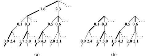
Figure 1: Matching on a PWIT, (a) with and (b) without root node. Numbers represent edge weights (lengths).

Consider a matching on an instance of a rooted PWIT, as well as a matching on the same instance but with the root removed, as shown in Fig. 1. Introduce the variable

$$X =$$ length of optimal matching on tree with root

$$- \mbox{length of optimal matching on tree without root}.$$

Both lengths are infinite, so this is interpreted as a limit of finite differences. If $X_{i}$ is the analogous quantity for the $i$th constituent subtree of the rootless PWIT instance and $\xi_{i}$ the length of the root’s $i$th edge, these variables satisfy the recursion

$$X=\min_{1\leq i<\infty}(\xi_{i}-X_{i}).$$ (1)

Now take the $\{\xi_{i}\}$ to be the Poisson-distributed edge lengths and the $\{X_{i}\}$ to be independent random variables from the same random process that produces $X$. Eq. (1) is then a distributional equation for $X$, and can be shown me94 for $d=1$ to have as its unique solution the logistic distribution

$$P(X\leq x)=\frac{1}{1+e^{-x}},\quad-\infty<x<\infty.$$ (2)

The PWIT structure further leads to the following inclusion criterion. Consider an edge of length $x$ in the tree, and the two subtrees formed by deleting that edge. The memoryless nature of the Poisson process allows us to consider each of these subtrees as independent copies of a PWIT, with their roots at the vertices of the deleted edge. It may be seen that including the edge in the optimal matching incurs a cost of $x-X_{1}-X_{2}$, where $X_{1}$ and $X_{2}$ are the $X$ variables as defined above, but for the two subtrees. Thus, an edge of length $x$ is present in the minimal matching if and only if

$$x<X_{1}+X_{2}.$$ (3)

The probability density function for edge lengths in the minimal matching is then

$$f(x)=P(x<X_{1}+X_{2}),\quad 0<x<\infty.$$

Here $X_{1}$ and $X_{2}$ are independent random variables distributed according to Eq. (2), from which the mean edge length can be calculated:

$$\int_{0}^{\infty}x\,P(x<X_{1}+X_{2})\,dx=\pi^{2}/6.$$

Mean-field MM and TSP

The previous section summarized analysis from  me94 ; now we continue with new analysis. To study scaling exponents, we introduce a parameter $\lambda>0$ that plays the role of a Lagrange multiplier. Penalize edges used in the optimal matching by adding $\lambda$ to their length. Let us study optimal solutions to the MM problem on this new penalized instance. Precisely, on a realization of the PWIT, define $Y$ and $Z$ as

length of optimal matching on new tree with root

$$-$$ length of optimal matching on new tree without root

where $Y$ and $Z$ differ in the definition of the edge lengths of the new tree: for $Y$, the edges penalized are those employed by the original rooted optimal matching; for $Z$, they are those employed by the original rootless optimal matching.

For the penalized problem the recursion Eq. (1) for $X$ is supplemented by the following recursions for $(X,Y,Z)$ jointly. Let $i^{*}$ be the value of $i$ that minimizes $\xi_{i}-X_{i}$. Then

$$Y = \min_{i}(\xi_{i}-(Z_{i}+\lambda)\,1(i=i^{*})-Y_{i}\,1(i\neq i^{*}))$$

$$Z = \min_{i}(\xi_{i}-Y_{i})$$

where, as before, the $\{Y_{i}\}$ and $\{Z_{i}\}$ are independent random variables from the same random process producing $Y$ and $Z$.

Moreover, we get an inclusion criterion, analogous to Eq. (3): an edge of length $x$ is included if and only if

$$x+\lambda<Z_{1}+Z_{2}$$ if edge used in optimal matching

$$x<Y_{1}+Y_{2} \ \mbox{ if edge not used in optimal matching}.$$

In terms of the expected unique joint distribution for $(X,Y,Z)$, the quantities $\delta$ and $\varepsilon$ that compare the penalized solution (as a non-optimal solution of the original problem) with the original optimal solution are

$$\delta(\lambda) = \int_{0}^{\infty}P\{\mbox{edge of length $x$ is in optimal penalized}$$

$$\qquad\mbox{matching but not in optimal matching}\}\,dx$$

$$= \int_{0}^{\infty}P(X_{1}+X_{2}<x<Y_{1}+Y_{2})\,dx$$

and

$$\varepsilon(\lambda) = \int_{0}^{\infty}x\,P\{\mbox{edge of length $x$ is in optimal penalized}$$

$$\qquad\mbox{matching}\}\,dx-\pi^{2}/6$$

$$= \int_{0}^{\infty}x\,[P(x<X_{1}+X_{2},\ x<Z_{1}+Z_{2}-\lambda)$$

$$\qquad+\ P(X_{1}+X_{2}<x<Y_{1}+Y_{2})]\,dx-\pi^{2}/6.$$

By the theory of Lagrange multipliers these functions $\varepsilon(\lambda),\delta(\lambda)$ determine $\varepsilon(\delta)$. We do not have explicit analytic expressions analogous to Eq. (1) for the joint distribution of $(X,Y,Z)$ in terms of $\lambda$. However, we can use routine bootstrap Monte Carlo simulations to simulate the distribution and thence estimate the functions $\delta(\lambda)$ and $\varepsilon(\lambda)$ numerically. And as indicated in  me94 sec. 6.2 and KM87 ; Cerf , the mean-field MM and the mean-field TSP can be studied using similar techniques; the TSP analysis is just a minor variation of the MM analysis. For instance, recursion Eq. (1) becomes

$$X={\min_{1\leq i<\infty}}^{[2]}(\xi_{i}-X_{i})$$

where $\min^{[2]}$ denotes second-minimum.

Table 1 reports numerical results showing good agreement with $\varepsilon\propto\delta^{3}$ in both problems for $d=1$. These numerics are compatible with independent MM results obtained recently Ratieville , as well as with our direct simulations on mean-field TSP instances at $n=512$. The same exponent $3$ arises for other $d$.

Table 1: Scaling for mean-field MM and TSP in pseudo-dimension $d=1$, obtained by simulating joint distribution of $(X,Y,Z)$. Results show a good fit to $\varepsilon\sim 2.3\delta^{3}$ and $2.0\delta^{3}$. In more detail, $\delta$ scales as $\lambda^{1/2}$ while $\varepsilon$ scales as $\lambda^{3/2}$. Estimates for $\varepsilon$ have standard deviation about $0.001$ for MM and $0.003$ for TSP.

					MM							TSP
$\lambda$			$\delta$		$\varepsilon$		$2.3\delta^{3}$			$\delta$		$\varepsilon$		$2.0\delta^{3}$
0.02			0.112		0.004		0.003			0.128		0.009		0.006
0.04			0.156		0.010		0.009			0.175		0.015		0.011
0.06			0.190		0.017		0.016			0.212		0.023		0.019
0.08			0.219		0.024		0.024			0.243		0.030		0.029
0.10			0.244		0.035		0.033			0.270		0.042		0.039
0.12			0.267		0.042		0.044			0.300		0.053		0.051
0.14			0.287		0.053		0.054			0.318		0.065		0.064
0.16			0.306		0.067		0.066			0.340		0.077		0.079
0.18			0.323		0.080		0.078			0.360		0.091		0.093
0.20			0.340		0.089		0.090			0.379		0.104		0.109

Euclidean MM and TSP

We consider the $d=1$ case where the scaling exponent can be found exactly, and give numerical results for other cases. We restrict the discussion to the Euclidean TSP, although as for the mean-field model, MM is phenomenologically similar.

Take the Euclidean TSP in $d=1$, with periodic boundary conditions. The optimal tour here is trivial (with high probability a straight line of length $n$) but nevertheless instructive to analyze. As before, add a penalty term $\lambda$ to each edge used in the tour, and consider how the optimal tour changes in this new penalized instance. When $\lambda$ is small, changes to the tour will consist of “2-changes” shown in Fig. 2, and will occur when an original edge length is less than $\lambda$. A simple nearest-neighbor distance argument gives the distribution of edge lengths in the original tour as $p(l)\sim e^{-l}$. Since two edges are modified in each 2-change,

$$\delta(\lambda)=2\int_{0}^{\lambda}p(l)\,dl\sim 2\lambda,\quad\varepsilon(\lambda)=2\int_{0}^{\lambda}l\,p(l)\,dl\sim\lambda^{2}.$$

The scaling exponent of 2 is not surprising, as the 1-d TSP behaves very similarly to the 1-d MST on penalized instances. Furthermore, it is consistent with the intuition that the “easiest” problems scale in this way. A similar argument applies to MM, and in both cases a more rigorous analysis yields bounds on $\delta$ and $\varepsilon$ that confirm the exponent.

Figure 2: “2-change” schematic. Original optimal tour is shown by dashed line. New optimal tour on penalized instance is shown by solid line: over sufficiently short lengths, tour doubles back to avoid using penalized edges.

For $d>1$, numerical results are shown in Fig. 3. These have been obtained by finding exact solutions to randomly generated $n=512$ Euclidean instances in $d=2,3,4$, using the Concorde TSP solver concorde . For each instance, the optimum was obtained on the original instance as well as on the instance penalized with a range of $\lambda$ values. For each $\lambda$ value, $\delta(\lambda)$ and $\varepsilon(\lambda)$ were averaged over the sample of instances. The resulting numerics are closely consistent with a scaling exponent of 3 (in spite of suffering from some finite-size effects at smaller $\delta$), suggesting that the mean-field picture gives the correct exponent in all but the trivial 1-dimensional case. In the language of critical exponents, this would correspond to an “upper critical dimension” of 2.

Figure 3: Scaling for Euclidean TSP in $d=2,3,4$, based on exact solutions for 100 instances in each case. Data points correspond to $\lambda$ values from 0.004 to 0.05. Slopes of best-fit lines vary from 2.94 to 3.24. Standard deviation is about $3\times 10^{-3}$ for $\delta$ and $3\times 10^{-5}$ for $\varepsilon$.

Discussion

The goal of our scaling study has been to address a new kind of problem in the theory of algorithms, using concepts from statistical physics. Traditionally, work on the TSP within the theory of algorithms TSPbook has emphasized algorithmic performance, rather than the kinds of questions we ask here. Rigorous study of the Euclidean TSP model within mathematical probability steele97 has yielded a surprising amount of qualitative information: existence of an $n\to\infty$ limit constant giving the mean edge-length in the optimal TSP tour BHH , and large deviation bounds for the probability that the total tour length differs substantially from its mean RT89 . However, calculation of explicit constants in dimensions $d\geq 2$ seems beyond the reach of analytic techniques. For the mean-field bipartite MM problem, impressive recent work LW03 ; NPS03 has proven an exact formula giving the expectation of the finite-$n$ minimum total matching length, though such exact methods seem unlikely to be widely feasible.

On the other hand, there has been significant progress over the past twenty years in the use of statistical physics techniques on combinatorial optimization problems in general. Finding optimal solutions to these problems is a direct analog to determining ground states in statistical physics models of disordered systems Moore87 . This observation has motivated the development of such approaches as simulated annealing KGV83 , the replica method MPV87 and the cavity method MPZ02 . Condensed matter physics, and particularly models arising in spin glass theory, has provided a powerful means to study algorithmic problems; at the same time, algorithmic results have implications for the associated physical models. It is instructive to consider our work in that context.

Researchers in the physical sciences have long been interested in the low-temperature thermodynamics MPV87 ; Dotsenko of disordered systems, investigating properties of near-optimal states in spin glass models. Our procedure for studying near-optimal solutions by way of a penalty parameter is similar to a method, known as $\epsilon$-coupling eps ; MPR-T , used for calculating low-energy excitations in spin glasses. Making use of this method, physicists have obtained quantities closely analogous to our scaling exponents for models of RNA folding MPR-T . Furthermore, in the last year independent work Ratieville has explored $\epsilon$-coupling on MM, numerically identifying a different but related scaling exponent.

For the TSP, analytical and numerical studies have been performed over fifteen years ago MP86 ; Sourlas on the thermodynamics of the model, with overlap quantities calculated for near-optimal solutions. The results have suggested that at low temperature $T$, the cost excess $\varepsilon$ scales as $T^{2}$ while the average fraction of differing edges between solutions ($1-q$, with $q$ being the “overlap fraction”) scales as $T$. This leads to $\varepsilon\sim(1-q)^{2}$, in apparent contradiction with our exponent of 3. However, at low temperatures, $q$ represents overlaps between typical near-optimal solutions, whereas our $\delta$ measures overlaps between a near-optimal solution and the optimum. The different definitions of these two quantities could account for the discrepancy in scaling exponent: it is not surprising that $1-q$ grows faster than $\delta$ as one considers solutions of increasing cost. At the same time, a possible implication of these results is that at low temperature, $\delta\sim T^{2/3}$. We are not aware of any direct theoretical arguments to explain this, and consider it an intriguing open question.

It is also important to note that the underlying property $\delta\to 0$ as $\varepsilon\to 0$ cannot always be taken for granted. This property is called asymptotic essential uniqueness (AEU) me94 . AEU requires, among other things, that the optimum itself be unique. In principal, even if it is not, one could still analyze near-optimal scaling by considering sufficiently local perturbations from a given optimum. It is natural to expect the resulting exponent to be independent of the specific optimum chosen. However, this may not be true in the event of what statistical physicists call replica symmetry breaking (RSB) MPV87 ; Dotsenko . AEU is a special case of replica symmetry, so while RSB implies the absence of AEU, the absence of AEU does not necessarily imply RSB. A current debate in the condensed matter literature concerns whether or not low-temperature spin glasses display RSB eps ; KM . It is generally believed that RSB is incompatible with unique non-zero values of various scaling exponents. Thus, the correct approach to analyzing near-optimal scaling in such problems remains another open question.

One final example may serve to illustrate the diversity of possible applications for our type of scaling analysis, as well as an instance where the absence of AEU is surmountable. In oriented percolation on the two-dimensional lattice, there are independent random traversal times on each oriented (up or right) edge. The percolation time $T_{n}$ is the minimum, over all ${2n\choose n}$ paths from $(0,0)$ to $(n,n)$, of the time to traverse the path. So $(2n)^{-1}E[T_{n}]\to t^{*}$, a time constant. It is elementary that there will be near-optimal paths, with lengths $T^{\prime}_{n}$ such that $n^{-1}(ET^{\prime}_{n}-ET_{n})\to 0$ and which are almost disjoint from the optimal path. So our $\varepsilon(\delta)$ analysis applied to paths will not be useful: even with a unique optimum, AEU will not hold. But we can rephrase the problem in terms of flows. A flow on the $n\times n$ oriented torus assigns to each edge a flow of size $\in[0,1]$, such that at each vertex, in-flow equals out-flow. Let $t(\delta)$ be the minimum, over all flows with mean flow-per-edge $=\delta$, of the flow-weighted average edge traversal time. In the $n\to\infty$ limit, one can show that as $\delta\to 0$, $t(\delta)\to t^{*}$ where $t^{*}$ is the same limiting constant as before. We therefore expect a scaling exponent $t(\delta)-t^{*}\sim\delta^{a}$. Mean field analysis meFPP gives $a=2$, and Monte Carlo study of the $d=2$ case is in progress.

Conclusions

We have studied the scaling of the relative cost difference $\varepsilon$ between optimal and near-optimal solutions to combinatorial optimization problems, as a function of the solution’s relative distance $\delta$ from optimality. This kind of scaling study, although well accepted in theoretical physics, is new to combinatorial optimization problems. For the MST, we have found $\varepsilon\sim\delta^{2}$. For the MM and TSP, in the 1-d Euclidean case $\varepsilon\sim\delta^{2}$ as well, while in both the mean-field model and higher Euclidean dimensions $\varepsilon\sim\delta^{3}$.

The scaling exponent may categorize combinatorial optimization problems into a small number of classes. The fact that MST is solvable by a simple greedy algorithm, and that the 1-d case of the MM and TSP is essentially trivial, suggests that a scaling exponent of 2 characterizes problems of very low complexity. The exponent of 3 characterizes problems that are algorithmically more difficult. Of course, this is a different kind of classification from traditional notions of computational complexity: MM is solvable to optimality in $O(n^{3})$ time whereas the TSP is NP-hard. Rather, these exponent classes are reminiscent of universality classes in statistical physics, which unite diverse physical systems exhibiting identical behavior near phase transitions.

A key question in the study of critical phenomena is whether mean-field models correctly describe phase transition behavior in the geometric models they approximate. The TSP and MM do not involve critical behavior, but the fact that mean-field and geometric scaling exponents coincide for $d\geq 2$ is significant. It provides evidence that in a combinatorial setting, the mean-field approach can give a valuable and accurate description of the structure of near-optimal solutions.

We thank Mike Steele for helpful discussions. David Aldous’s research is supported by NSF Grant DMS-0203062. Allon Percus acknowledges support from DOE LDRD/ER 20030137, as well as the kind hospitality of the UCLA Institute for Pure and Applied Mathematics where much of this work was conducted.

References

- (1) Dyer, M., Greenhill, C. & Molloy, M. (2002) Random Structures and Algorithms 20, 98–114.
- (2) Evans, W., Kenyon, C., Peres, Y. & Schulman, L.J. (2000) Annals of Applied Probability 10, 410–431.
- (3) Coppersmith, D., Gamarkin, D., Hajiaghayi, M.T. & Sorkin, G.B. (2003) in Proceedings of the 14th Annual ACM-SIAM Symposium on Discrete Algorithms (ACM, New York), 364–373.
- (4) Mézard, M., Parisi, G. & Zecchina, R. (2002) Science 297, 812–815.
- (5) Monasson, R., Zecchina, R., Kirkpatrick, S., Selman, B. & Troyansky, L. (1999) Nature 400, 133–137.
- (6) Aldous, D.J. & Steele, J.M. (2003) Asymptotic essential uniqueness and its scaling exponent for minimal spanning trees on random points, to be published.
- (7) Mézard, M. & Parisi, G. (1985) Journal de Physique Lettres 46, L771–L778.
- (8) Aldous, D.J. (2001) Random Structures and Algorithms 18, 381–418.
- (9) Aldous, D.J. & Steele, J.M. (2003) The objective method: Probabilistic combinatorial optimization and local weak convergence, to be published.
- (10) Krauth, W. & Mézard, M. (1987) Europhys. Lett. 8, 213–218.
- (11) Cerf, N.J., Boutet de Monvel, J., Bohigas, O., Martin, O.C. & Percus, A.G. (1997) Journal de Physique I 7, 117–136.
- (12) Ratiéville, M. (2002) Ph.D. thesis (Université Pierre et Marie Curie, Paris and Università degli Studi di Roma “La Sapienza”, Rome).
- (13) Applegate, D., Bixby, R., Chvátal, V. & Cook, W. Concorde, available at: www.math.princeton.edu/tsp/concorde.html.
- (14) Gutin, G. & Punen, A.P., eds. (2002) The Traveling Salesman Problem and its Variations (Kluwer, Dordrecht).
- (15) Steele, J.M. (1997) Probability Theory and Combinatorial Optimization (SIAM, Philadelphia).
- (16) Beardwood, J., Halton, J.H. & Hammersley, J.M. (1959) Proc. Cambridge Philos. Soc. 55, 299–327.
- (17) Rhee, W.T. & Talagrand, M. (1989) Ann. Probability 17, 1–8.
- (18) Linusson, S. & Wästlund, J. (2003) A proof of Parisi’s conjecture on the random assignment problem, math.CO/0303214.
- (19) Nair, C., Prabhakar, B. & Sharma, M. (2003) A proof of the conjecture due to Parisi for the finite random assignment problem, unpublished.
- (20) Moore, M.A. (1987) Phys. Rev. Lett. 58, 1703–1706.
- (21) Kirkpatrick, S., Gellatt, C.D. & Vecchi, M.P. (1983) Science 220, 671–680.
- (22) Mézard, M., Parisi, G. & Virasoro, M.A. (1987) Spin Glass Theory and Beyond (World Scientific, Singapore).
- (23) Dotsenko, V. (2001) Introduction to the Replica Theory of Disordered Statistical Systems (Cambridge University Press, Cambridge).
- (24) Palassini, M. & Young, A.P. (2000) Phys. Rev. Lett. 85, 3017–3020; Marinari, E. & Parisi, G. (2001) Phys. Rev. Lett. 86, 3887–3890.
- (25) Marinari, E., Pagnani, A. & Ricci-Tersenghi, F. (2002) Phys. Rev. E 65, 041919.
- (26) Mézard, M. & Parisi, G. (1986) Journal de Physique 47, 1285–1296.
- (27) Sourlas, N. (1986) Europhys. Lett. 2, 919–923.
- (28) Krzakala, F. and Martin, O.C. (2000) Phys. Rev. Lett. 85, 3013–3016.
- (29) Aldous, D.J. A non-rigorous scaling law in mean-field first passage percolation, in preparation.