Random Networks Growing Under a Diameter Constraint

Abstract

We study the growth of random networks under a constraint that the diameter, defined as the average shortest path length between all nodes, remains approximately constant. We show that if the graph maintains the form of its degree distribution then that distribution must be approximately scale-free with an exponent between $2$ and $3$. The diameter constraint can be interpreted as an environmental selection pressure that may help explain the scale-free nature of graphs for which data is available at different times in their growth. Two examples include graphs representing evolved biological pathways in cells and the topology of the Internet backbone. Our assumptions and explanation are found to be consistent with these data.

Measurements on a wide variety of networks such as the World Wide Webdiameter ; ladamicsw , the Internet backbone achilles_heel ; faloutsos99topology , social networks chung ; strogatz_review ; wattssw , and metabolic networksbarabasi ; fell have shown that they differ significantly from the classic Erdos-Renyi model of random graphs erdos . While the traditional Erdos-Renyi model has a Poisson node degree distribution, with most nodes having a characteristic number of links, these networks have highly skewed, scale-free degree distributions approximately following a power law $p(k)\sim k^{-\gamma}$, where $k$ is the node degree, and $\gamma$ is the scale-free exponent. To account for these observations, random graph growth models have been developed huberman_growth ; pref_attatch ; stoch_web ; krapivsky2000 ; dorogovtsevPRE2000 that rely on the intuitively appealing idea of preferential attachment.

For the most part, these models are of growing networks in which new nodes are added to a graph by addition of one or more edges to already existing nodes. The attachment is preferential because the likelihood of attachment to a node depends on the number of other nodes already linked to it. Thus, such models rely solely on endogenous factors, since they do not take account of any global exogenous selection pressures which might shape the form of evolving and growing networks.

Such selection pressures would be especially relevant, for example, in a biological context. Measurements of the topological properties of graphs representing the metabolic networks of $43$ organisms have demonstrated their scale-free nature barabasi ; metabolicproceedings . In all of these graphs, of different sizes, it was found that the diameter, defined as the average shortest path between every pair of nodes in the graph, was constant. Such a constancy may be related to important properties relevant to the core functioning of these biological networks, such as the spread and speed of responses to perturbations fell ; fellproceedings .

Another example is the Internet backbone graph, whose growth and evolution over time has been studied by several authors faloutsos99topology ; vespignaniPRLbackbone ; goh2002PRLtopology . In this case, there are performance and robustness constraints that such networks much satisfy. These constraints can be thought of as environmental pressures (which may operate indirectly) that would select against highly inefficient network structures. One possibility may be a bias in favor of network changes and additions that tend to maintain the average shortest path.

These two cases are relatively rare examples of network data representing graphs of varying size shaped by similar selection pressures, and they allow the testing of explanations for their generic features. The main selection-based explanation barabasi for scale-free network topologies relies on the fact that such networks are robust with respect to random malfunction of nodes achilles_heel . Robustness is identified with the diameter of the network, and scale-free networks maintain their diameter when nodes are eliminated at random. However, while scale-free graphs are robust in this sense, it has not been shown that robust graphs must necessarily be scale-free.

In this Letter, we argue that another notion of robustness can be added to the error tolerance argument. Namely, scale-free networks are special in the sense that they can grow, with the same functional form for the degree distribution, and simultaneously maintain an approximately constant diameter. This implies that when graphs grow and evolve in an environment in which there are selection pressures on the diameter, these graphs are likely to be scale-free. Our results help clarify the connection between the apparent constancy of the diameter and the scale-free topology of the graphs in the two examples studied.

We consider random graphs of different sizes under the constraint that the diameter remain approximately constant as the graph grows. We show that if the graph maintains the form of its degree distribution then that distribution must be approximately scale-free with an exponent between $2$ and $3$. These results may help explain the scale-free nature of graphs, of varying sizes, representing the evolved metabolic pathways of different organisms and the topology of the Internet backbone. Our assumptions and results are consistent with empirical findings.

We start with an expression for the diameter $d$ of a random graph with arbitrary degree distribution developed in Ref. newman01graphs using a generating function formalism applied to the degree distribution $p\left(k\right)$,

$$d=\frac{\log N}{\log(z_{2}/z_{1})}-\frac{\log z_{1}}{\log(z_{2}/z_{1})}+1$$ (1)

This formula depends only on the number of nodes in the graph $N$, the average degree of the nodes $z_{1}$, and the average number of nodes $z_{2}$ that are reachable in two edge traversals from an arbitrary node. The formula was derived by considering an ensemble of random graphs (without explicit clustering, see Refs. newman01graphs ; newmanchapter for details), and calculating from the degree distribution the average number of nodes within some radius of edges away from a random node. As the radius gets larger, the number of nodes enclosed grows rapidly. When that number of nodes is approximately equal to $N$, the corresponding radius is a good approximation to the average shortest path in the graph, since most of the nodes are at that distance. If the random graph is directed, the same argument applies, and Eq. (1) is valid when $p\left(k\right)$ is the degree distribution of outgoing edges.

It is important to emphasize that Eq. (1) is an approximate formula for the average shortest path of a random graph (without clustering or assortative mixing, etc.). While the formula is not numerically precise, it does capture the dependence of the diameter on $N$.

To calculate the diameter of a graph with degree distribution $p\left(k\right)$, but with a finite number of nodes $N$, the size of the graph must be parameterized through the degree distribution. In any fully connected finite-sized graph, the smallest possible degree is $1$ and the largest degree in the graph must be less than $N$. The parameterization can be accomplished by imposing an $N$-dependant cutoff function $k_{c}\left(N\right)<N$ and writing $\left<k^{i}\right>=\sum_{1}^{k_{c}\left(N\right)}k^{i}p\left(k\right)$.

Additionally, a simple application of the generating function method leads to the relationship $z_{2}=\left<k^{2}\right>-\left<k\right>$ ($\left<k\right>=z_{1}$ by definition), which allows the diameter to be calculated from the first two moments of $p\left(k\right)$.

We seek a degree distribution that maintains its functional form and has an approximately constant diameter independent of $N$. Effectively, this means a single function $p\left(k\right)$ that does not depend on $k_{c}$ except through its normalization. (We rule out the most obvious example, a star-shaped graph with $N-1$ nodes each connected to the $N$th node. This graph, whose construction is deterministic, has an approximately constant diameter of $2$.)

Returning to Eq. (1), consider the first and second terms. The first plus the third term are an upper bound on $d$ since the second term is strictly non-negative and always $\leq 1$. In addition, for any fixed $p\left(k\right)$, the second term is non-increasing as $k_{c}$ gets larger, and will approach a constant $\leq 1$ if $p\left(k\right)$ has finite moments as $N\rightarrow\infty$. As a result, for our purposes the first term is dominant, and we will neglect the second. If the first term is a constant $c$, then the diameter will always lie between $c$ and $c+1$.

Thus, in order to find the degree distribution with approximately constant diameter independent of $N$, we set the first term in Eq. (1) be equal to a constant $c$, which results in the requirement that

$$N^{1/c}=z_{2}/z_{1}$$ (2)

The ratio $z_{2}/z_{1}$ is also the average degree of a node found by following a randomly chosen edge newman01graphs . This average degree must always be less than the largest degree in the graph, which provides a lower bound on the cutoff function $k_{c}\left(N\right)$, resulting in $N^{1/c}<k_{c}\left(N\right)<N$ for all $N$. The function $k_{c}\left(N\right)$ is therefore bounded from above and below by power functions and we will use the explicit form $k_{c}\left(N\right)=N^{\alpha}$ where $1/c<\alpha\leq 1$. Setting $\alpha=1$, we recover the least restrictive case where no node has a degree greater the size of the graph. Letting $\alpha$ vary also allows us to see the consequences of different cutoff dependencies if they are consistent with empirical findings.

Then, using again the assumption $N\gg 1$, Eq. (2) can be written as an equation for $p\left(k\right)$ involving the ratio of its moments:

$$k_{c}^{\frac{1}{\alpha c}}=\frac{\sum_{1}^{k_{c}}k^{2}p\left(k\right)}{\sum_{1}^{k_{c}}kp\left(k\right)}$$ (3)

The distribution $p(k)$ can be determined by writing this equation for $k_{c}$ and $k_{c}\pm 1$. Algebraic manipulation yields the recurrence relation

$$p(k+1)=p(k)\frac{k^{2}-k(k-1)^{\beta}}{(k+1)^{2}-(k+1)^{\beta+1}}\frac{(k+1)^{\beta}-k^{\beta}}{k^{\beta}-(k-1)^{\beta}}$$ (4)

where $\beta\equiv 1/\alpha c$ for convenience. The full solution can easily be calculated numerically. For most values of $\beta$ the distribution approaches its scale-free asymptote rather quickly (by $~{}k=100$), as shown in Fig. 1.

Figure 1: A plot of the numerically calculated distributions for various values of $\beta$ and with a $k_{max}=10^{4}$.

A more explicit analytic characterization of the solution can be found by using an integral approximation for Eq. (4), $k_{c}^{\frac{1}{\alpha c}}=\frac{\int_{1}^{k_{c}}k^{2}p\left(k\right)dk}{\int_{1}^{k_{c}}kp\left(k\right)dk}$ This integral equation can be solved exactly by turning it into a first-order differential equation for the function $p\left(\cdot\right)$ by differentiations with respect to $k_{c}$. Replacing $k_{c}$ with a dummy variable $k$, and writing $\beta=1/\alpha c$ for convenience, the resulting equation is $((\beta-3)k+(\beta+2)k^{\beta})p\left(k\right)+k(k^{\beta}-k)p^{\prime}\left(k\right)=0$. The unique solution, up to a normalization constant dependent on $k_{c}$, is

$$p\left(k\right)=\frac{1}{k^{3-\beta}}(1-\frac{1}{k^{1-\beta}})^{\frac{1-2\beta}{\beta-1}}$$ (5)

The solution is in good agreement with the result of numerical iteration of the exact result of Eq. (4) away from $k=1$. The singular behavior for $\beta<1/2$ at $k=1$ is the result of the continuous approximation. Nevertheless, Eq. (5) well approximates the form of the distribution with an approximately constant diameter that is always between $c$ and $c+1$, approaching $c+1$ asymptotically with $N$. For $k\gg 1$, it is also a scale-free distribution with exponent $\gamma=3-1/\alpha c$. Since $\alpha>1/c$ and $c\geq 1$ is a natural bound on $c$, the scale-free exponent satisfies $2<\gamma<3$, and it can be written in terms of the diameter $d$ and the cutoff exponent $\alpha$ as $\gamma=3-\frac{1}{\alpha(d-1)}$.

These results are valid for the model of random graphs constructed according to the simple method assumed in Ref. newman01graphs . Even for these ideal graphs, Eq. (1) numerically underestimates the actual path lengths, as is obvious from its method of derivation, but it does capture the proper scaling behavior. Real-world graphs with additional non-random structure can have even longer average shortest paths. Nevertheless, as shown in albert02review ; newmanchapter ; newman_scientific_collabII , the formula does approximate the diameter for many real-world graphs, especially with respect to the dependence of the average path length on $N$. In our experiments on two diverse real-world data sets, we also find the numerical underestimation. Still, a comparison between the behavior of Eq. (1) and measured diameters on our data sets for all $N$ shows that this analytical treatment tracks the basic features of the data quite well (see Figs. 2a and 3a).

We next consider our assumptions and results in the context of two data sets, each representing snapshots of the topologies of graphs that grow in an environment with possible selection pressures. The first concerns the organization of essential biological processes within the cell for a variety of simple organisms, and the second concerns the large-scale structure of the Internet backbone. While these are, of course, very different examples, we will show that they do share features consistent with the arguments just presented, and we provide reasons for why a selection argument related to the diameter of these networks is reasonable.

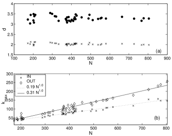
Figure 2: (a) The diameter $d$ is almost constant as a function of $N$, the size of the metabolic network. The top set of points are the measured average shortest path on the graphs, while the bottom set shows the quantity computed from the degree distributions using Eq. (1). (b) The maximum in degree and out degree of the node scales linearly with the size of the network.

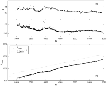
Figure 3: (a) Evolution of the Internet backbone diameter with the number of nodes recorded on NLANR Internet maps. The top curve is the measured average shortest path on the graphs, while the bottom panel shows the quantity computed from the degree distributions using Eq. (1). Days where the mapping was incomplete are omitted. (b) The maximum degree of a node scales linearly with the size of the network.

Metabolic pathways are complex biological networks in which a series of enzymatic reactions produce specific products within cells. Large scale sequencing projects have furnished integrated pathway-genome databaseskarp ; kanehisa ; wit from which organism-specific metabolic networks can be inferred. In a metabolic network, nodes represent the substrates, and a directed link connects the educt to the product of a metabolic reaction.

Recently, such databases have been used barabasi ; fell to analyze the topological properties of the metabolic networks of $43$ different organisms including E-coli (bacterium) and Caenorhibditis elegans (eukaryote). The network degree distributions were found to be uniformly scale-free with exponents between $2.0$ and $2.4$. A striking feature of the metabolic networks studied is that even though their sizes vary between 200 and 800 nodes, the diameter stays approximately fixed between $3.0$ and $3.5$, as shown in Fig. 2a.

It has been speculated fell ; fellproceedings that metabolic networks may have evolved to maintain a constant diameter in order to minimize the number of sequential reactions necessary to obtain a particular product. For example, it was found that there are several possible pathways which could provide the same chemical solution as the Krebs cycle, but the true Krebs cycle is the most efficient and contains the least number of steps enrique . Another possible evolutionary force is opportunism, where a new metabolic pathway is developed by re-using enzyme catalyzing reactions already in the cell rather than developing an entirely new pathway from scratch fell . Thus, as the network evolves, existing substrates are incorporated into new pathways and their connectivity grows. Fig. 2b shows that the degree of the most connected node grows linearly with the size of the metabolic network, in agreement with the assumption $k_{c}\sim N^{\alpha}$.

Further potential benefits of small diameters include the reduction in the transition time between metabolic states fell in response to environmental changes. Networks with robustly small average path lengths have been found to rapidly adjust to perturbations wattssw . Thus there may be a selective advantage to maintaining a small diameter.

The Internet backbone is a second example of a network where maintaining a constant diameter is important. Data is routed on the Internet between tens of millions of host computers by breaking the data up into packets, each of which are routed individually and then re-assembled upon arrival at their destination. The packets hop from node to node in the network. Each additional hop a packet must make introduces latency and increases the potential for signal degradation through errors and delays. We measured the diameter of Internet maps from November 1997 to January 2000 gathered by the National Laboratory for Applied Network Research (NLANR)(http://moat.lanr.net). Each node is an autonomous system (AS) usually corresponding to a single Internet Service Provider, and the links represent inter-ISP connections. The Internet backbone connectivity distribution is power-law with an exponent $\gamma=2.2\pm 0.1$ invariant over time vespignaniPRLbackbone ; faloutsos99topology . An example degree distribution is shown in Fig. 4 along with a distribution calculated using the recursion in Eq. (4). Fig. 3a shows, consistent with previous measurements vespignaniPRLbackbone , that the diameter stays approximately constant at 3.7 hops over the 2 year period, while the number of nodes doubles from three to six thousand. It appears that the Internet backbone may have evolved to connect a greater number of ISPs but has kept the average number of hops Internet traffic must make low.

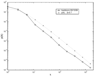
Figure 4: An example degree distribution for the Internet backbone compared with a distribution computed using the recursion in Eq. (4).

In summary, we have presented a plausible reason for the existence of scale-free distributions observed in two contexts, metabolic networks and the Internet backbone, where there are evolutionary pressures to maintain a small diameter. Our analysis shows that for a robust network to maintain its diameter, the form of its degree distribution should be scale-free. We have further shown our assumptions to be consistent with observed features in the two data sets. Combined with endogenous models of preferential attachment, and the error tolerance of scale-free networks, our results help further explain the prevalence of scale-free networks in selective environments.

We acknowledge B. A. Huberman for many useful discussions and A. R. Puniyani for contributions to earlier versions of this work.

References

- (1) H. Jeong, R. Albert, and A. L. Barabasi, Nature 401, 130 (1999).
- (2) L. Adamic, in Proceedings of ECDL’99, Lecture Notes in Computer Science 1696 (Springer, ADDRESS, 1999), pp. 443–452.
- (3) R. Albert, H. Jeong, and A.-L. Barabasi, Nature 406, 378 (2000).
- (4) M. Faloutsos, P. Faloutsos, and C. Faloutsos, in ACM SIGCOMM (PUBLISHER, ADDRESS, 1999), pp. 251–262.
- (5) W. Aiello, F. R. K. Chung, and L. Lu, ACM Symposium on Theory of Computing 171 (2000).
- (6) S. Strogatz, Nature 410, 268 (2001).
- (7) D. J. Watts and S. Strogatz, Nature 393, 440 (1998).
- (8) H. Jeong et al., Nature 407, 651 (2000).
- (9) A. Wagner and D. Fell, Nature Biotechnology 18, 1121 (2000).
- (10) P.Erdos and A.Renyi, Pupl. Math. Inst. Hungar. Acad. Sci. 7, 17 (1960).
- (11) B.A.Huberman and L. Adamic, Nature 401, 131 (1999).
- (12) A.-L. Barabasi and R. Albert, Science 286, 509 (1999).
- (13) P. Raghavan et al., Proceedings of the IEEE Symposium on Foundations of Computer Science (2000).
- (14) P.L.Krapivsky, S.Redner, and F.Leyvraz, Physical Review Letters 85, 4629 (2000).
- (15) S.N.Dorogovtsev and J.F.F.Mendes, Physical Review E 62, 1842 (2000).
- (16) H. Jeong, A.-L. Barab si, B. Tombor, and Z. N. Oltvai, in Proceeding of 2nd Workshop on Computation of Biochemical Pathways and Genetic Networks, edited by R. Gauges, C. van Gend, and U. Kummer (Logos Verlag, ADDRESS, 2001).
- (17) D. A. Fell and A. Wagner, in Animating the cellular map, edited by J.-H. S. Hofmeyr, J. M. Rohwer, and J. L. Snoep (Stellenbosch University Press, Stellenbosch, ADDRESS, 2000), pp. 79–85.
- (18) R. Pastor-Satorras, A. V zquez, and A. Vespignani, Physical Review Letters 87, 258701 (2001).
- (19) K. Goh, B. Kahng, and D. Kim, Physical Review Letters 88, 108701 (2002).
- (20) M. E. J. Newman, S. H. Strogatz, and D. J. Watts, Phys. Rev. E 64, 026118 (2001).
- (21) M. E. J. Newman, in Handbook of Graphs and Networks, edited by S. Bornholdt and H. G. Schuster (Wiley-VCH, Berlin, 2002), Chap. Random Graphs as Models of Networks, to appear.
- (22) R. Albert and A.-L. Barabasi, Review of Modern Physics 74, 47 (2002).
- (23) M. Newman, Phys. Rev. E 64, 016132 (2001).
- (24) P. Karp, M. Krummenacker, S. Paley, and J. Wagg, Trends Biotech 17, 275 (1999).
- (25) M. Kanehisa and S. Goto, Nucleic Acid Res 28, 27 (2000).
- (26) R. Overbeek et al., Nucleic Acids Res. 28, 123 (2000).
- (27) E. M. Hevia, M. Cascante, and T. Wadell, Journal of Theoretical Biology 166(2), 201 (1994).
- (28) F. R. K. Chung and L. Lu, Proceedings of the National Academy of Sciences, to appear 10.1073/pnas.252631999, (2003).
- (29) M. E. J. Newman, D. J. Watts, and S. H. Strogatz, Proc. Natl. Acad. Sci. 99, 2566 (2002).