Communication near the channel capacity with an absence of compression:
Statistical Mechanical Approach

Abstract

The generalization of Shannon’s theory to include messages with given autocorrelations is presented. The analytical calculation of the channel capacity is based on the transfer matrix method of the effective 1D Hamiltonian. This bridge between statistical physics and information theory leads to efficient Low-Density Parity-Check Codes over Galois fields that nearly saturate the channel capacity. The novel idea of the decoder is the dynamical updating of the prior block probabilities which are derived from the transfer matrix solution and from the posterior probabilities of the neighboring blocks. Application and possible extensions are discussed, specifically the possibility of achieving the channel capacity without compression of the data.

Digital communication, which is the driving force of the modern information revolution, deals with the task of achieving reliable communication over a noisy channel. A typical communication channel is depicted in figure 1 (where $K\leq L$ and $K\leq N$).

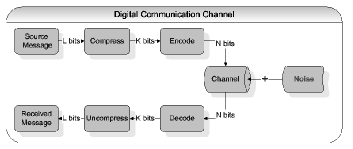
Figure 1: Digital Communication Channel

Shannon, in his seminal workShannon-48 , proved that in order to overcome noise, redundancy must be added to the transmitted message. The channel capacity, which is the maximal rate ($R\equiv\frac{K}{N}$) is a function of the channel bit error rate ($f$), bit error rate ($P_{b}$) and the a priori bit probability ($P$)

$$R=\frac{1-H_{2}\left(f\right)}{H_{2}\left(P\right)-H_{2}\left(P_{b}\right)}$$ (1)

where $H_{2}\left(x\right)\equiv-x\log_{2}\left(x\right)-\left(1-x\right)\log_{2}\left(1-x\right)$. The entropy, defined as the information content (in bits per symbol) of the message, is unity for unbiased ($P=0.5$) messages and decreases with bias ($H_{2}\left(0\right)=H_{2}\left(1\right)=0$).

To maximize channel throughput, the message is first compressed using algorithms (e.g., LZ78 ) which approach entropy for large blocks, and then encoded assuming a unbiased message. Typical messages exhibit low autocorrelation coefficients (decreasing with the size of the message)lacs . For instance, the discrete periodic 2-point autocorrelation coefficient of a sequence $\left\{X_{i}\right\}$ is defined by

$$C_{k}=\frac{1}{L}\sum_{i=1}^{L}X_{i}X_{\left(i+k\right)\>\mathbf{mod}\>L}$$ (2)

Compressible data exhibits enhanced autocorrelation coefficients, whose distribution has been extensively studied in numerous fields (e.g., linguistics, DNA research, heartbeat intervals, etc.)zipf ; Havlin .

In this paper we raise two questions:

• what is the channel capacity of correlated sequences?

• are these bounds achievable by an encoder alone, without the preceding compression phase?

We address these questions by using models from statistical mechanics, which lead to a new class of decoding algorithms. The decoder nearly approaches the capacity expected for perfect compression, without directly applying any compression.

The motivation for direct transmission of the uncompressed data is to overcome many difficulties, including:

• a single bit error in a compressed block would render the entire block useless. This is particularly important for applications where minimal distortion can be tolerated (e.g., audio/video transmission)

• compression of different packets of the same length would generate different length output messages, calling for greater complexity of the encoder

• the compression/decompression add delay to each transmission, and increase the complexity of the transmitter/receiver.

We start by calculating the entropy of correlated bit sequences. This is done by binning the source into $K_{o}$ bits, where $K_{o}$ is the highest autocorrelation coefficient taken, and using the transfer-matrix method. We proceed by integrating the results of the transfer matrix into a new decoding algorithm, based on a Low-Density Parity-Check Codes (LDPCC) over finite fields ($GF\left(q\right)$)LDPC-GF(q) .

For the sake of simplicity, we begin by demonstrating the entropy calculation for two autocorrelation coefficients, namely, $C_{1}$ and $C_{2}$. The entropy of a set of binary sequences of length $L$ is defined by the log of the number of possible sequences ($\Omega$) divided by $L$. Calculating $\Omega$ with the correlation constraints ($C_{1}$, $C_{2}$)sourlas , is done by taking the trace over all possible states of the sequence obeying the constraints imposed as delta functions

$$\Omega=\mathop{\rm Tr}\delta\left(\sum_{j}x_{j}x_{j+1}-C_{1}L\right)\delta\left(\sum_{j}x_{j}x_{j+2}-C_{2}L\right)$$ (3)

where periodic boundary conditions are assumed for the indices. Using the Fourier representation of the delta functions and rearranging terms, one gets

$$\Omega = \frac{1}{\left(2\pi\right)^{2}}\int\int_{-\infty}^{\infty}\mathbf{d}y_{1}\mathbf{d}y_{2}e^{-iL\left(y_{1}C_{1}+y_{2}C_{2}\right)}$$ (4)

$$\times\mathop{\rm Tr}\prod_{j=1}^{\frac{L}{2}}e^{iB\left(y_{1},y_{2},x_{2j}\ldots x_{2j+3}\right)}$$

where $B$ is given by

$$B\left(y_{1},y_{2},x_{0},x_{1},x_{2},x_{3}\right) \equiv \frac{y_{1}}{2}\left(x_{0}x_{1}+2x_{1}x_{2}+x_{2}x_{3}\right)$$ (5)

$$+y_{2}\left(x_{0}x_{2}+x_{1}x_{3}\right)$$

Using the transfer-matrix methodbaxter-TM , we group the sequence into blocks of 2 bits, obtaining the 4x4 matrix

$$V\left(y_{1},y_{2}\right)=\left(\begin{array}[]{cccc}e^{2y_{1}+2y_{2}}&e^{y_{1}}&e^{-y_{1}}&e^{-2y_{2}}\\ e^{-y_{1}}&e^{-2y_{1}+2y_{2}}&e^{-2y_{2}}&e^{y_{1}}\\ e^{y_{1}}&e^{-2y_{2}}&e^{-2y_{1}+2y_{2}}&e^{-y_{1}}\\ e^{-2y_{2}}&e^{-y_{1}}&e^{y_{1}}&e^{2y_{1}+2y_{2}}\end{array}\right)$$ (6)

representing all possible interactions between neighboring blocks. We proceed by replacing the trace with $\lambda_{{}_{max}}^{{}^{\frac{L}{2}}}$, where $\lambda_{max}$ is the principal eigenvalue of $V\left(y_{1},y_{2}\right)$. Using the method of Laplace integrals we obtain for the leading orderprl-referee of $\Omega$

$$\Omega=e^{-L\left(y_{1}^{\star}C_{1}+y_{2}^{\star}C_{2}-\frac{1}{2}\ln\lambda_{max}\left(y_{1}^{\star},y_{2}^{\star}\right)\right)}$$ (7)

where $\left(y_{1}^{\star},y_{2}^{\star}\right)$ are the solution of the saddle point equations. The entropy in bits is given by

$$H\left(C_{1},C_{2}\right)=\frac{\frac{1}{2}\ln\lambda_{max}\left(y_{1}^{\star},y_{2}^{\star}\right)-y_{1}^{\star}C_{1}-y_{2}^{\star}C_{2}}{\ln 2}$$ (8)

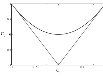
Figure 2: Phase space for sequences with $C_{1},C_{2}$. Outside the triangle ($\left|C_{1}\right|\geq\frac{1+\left|C_{2}\right|}{2}$) the entropy is zero. The parabolic curve is $C_{2}=C_{1}^{2}$.

The entropy of the correlated sequences are shown in figure 2 for all possible {$C_{1},C_{2}$} tuples. The area of non-zero entropy is depicted in figure 2 between the two straight lines, i.e., $\frac{-1-C_{2}}{2}<C_{1}<\frac{1+C_{2}}{2}$. The parabolic line is $C_{2}=C_{1}^{2}$, where the entropy reduces to the case of a single $C_{1}$ constraint, with the entropy $S=H_{2}\left(\frac{1+C_{1}}{2}\right)$C1-gauge . This is the typical case for the $C_{1}$ constraint, since $C_{2}$ can be viewed as multiplying two consecutive $C_{1}$ pairs, hence it has the highest entropy for a given $C_{1}$.

Note that at the boundary of the phase space the entropy falls abruptly to zero (a first order phase transition). Another point, which might appear counter-intuitive, is the fact that the entropy of the constraint {$C_{1}=A,C_{2}=B$} is not the same as {$C_{1}=B,C_{2}=A$} corr-cluster .

The transfer-matrix solution shows that the ensemble of sequences obeying the correlation constraints are obtained from the thermal equilibrium solution of the 1-D Ising spin model (where the two states of the spin correspond to the binary values of the bit $\left\{0,1\right\}\rightarrow\left\{1,-1\right\}$ sourlas ). The interaction length is the same as the correlation length, and the interaction strength is $J_{i}=-\frac{y_{i}^{\star}}{\beta}$ (where $\beta$ is the inverse temperature). The corresponding Hamiltonian is $H=-\frac{y_{1}^{\star}}{\beta}\sum x_{i}x_{i+1}-\frac{y_{2}^{\star}}{\beta}\sum x_{i}x_{i+2}$. This physical observation is the key leading to our novel decoding algorithm.

Testing the physical mapping, we choose a pair of constraints ($C_{1},C_{2}$), solve the transfer matrix model to obtain $y_{1}^{\star},y_{2}^{\star}$, then select any temperature (e.g., $\beta=1$) which gives the interactions $J_{1},J_{2}$frustrated_interactions , and perform Monte-Carlo simulations, and indeed the system settles into an equilibrium state obeying the initial autocorrelation constraints.

The division into blocks of 2 bits, amplifies the fact that interactions affect only neighboring blocks, and the probability of finding a block in one of its four possible states depends only on the state of its two neighbors. Labeling the left, center and right blocks by $l,c,r$ respectively, one gets for the joint probability of three consecutive blocks

$$P\left(c,l,r\right)=\frac{S_{I}\left(c\right)q_{L}^{l}S_{L}\left(l,c\right)q_{R}^{r}S_{R}\left(r,c\right)}{\mathop{\rm Tr}_{\left\{c,l,r\right\}}S_{I}\left(c\right)q_{L}^{l}S_{L}\left(l,c\right)q_{R}^{r}S_{R}\left(r,c\right)}$$ (9)

where

$$S_{I}\left(c\right) = e^{y_{1}^{\star}c_{1}c_{2}}$$

$$S_{L}\left(l,c\right) = e^{y_{1}^{\star}l_{2}c_{1}+y_{2}^{\star}\left(c_{1}l_{1}+c_{2}l_{2}\right)}$$ (10)

$$S_{R}\left(r,c\right) = e^{y_{1}^{\star}c_{2}r_{1}+y_{2}^{\star}\left(c_{1}r_{1}+c_{2}r_{2}\right)}$$

The first term in Equation 10 denotes the inner-block interactions, and the other terms denote the inter-block interactions. $q_{L}^{l}$/$q_{R}^{r}$ is the posterior probability of finding the left/right block in a specific state given by the decoding algorithm below, and the subscripts 1,2 denote the bit number in the block.

The physical spin model emphasizes the dramatic difference between the case of biased bit probabilities, equivalent to an induced homogeneous field, where each spin is updated independently, to the case of correlations induced by inter-spin interactions.

The entropy of the class of correlated sequences, derived by the transfer-matrix method, can be plugged into equation 1. Using shannon’s lower bound, gives the channel capacity of sequences with two autocorrelation coefficients

$$R^{\star}=\frac{1-H_{2}\left(f\right)}{H_{2}\left(C_{1},C_{2}\right)-H_{2}\left(P_{b}\right)}$$ (11)

The previous formulation is easily extended to higher autocorrelation coefficients. The procedure involves adding more delta functions to equation 3, resulting in a larger transfer matrix. For $C_{l}$ , being the highest autocorrelation coefficient, one gets $l$ variables ($y_{1}\ldots y_{l}$), and a transfer matrix’s dimension is $2^{l}\times 2^{l}$, which is solved numerically. The simulation results, shown in this paper, were conducted on sequences with 2 ($C_{1},C_{2}$), and 3 ($C_{1},C_{2},C_{3}$) autocorrelation constraints.

Equation 9 is the crux of our decoding algorithm, it enables the decoder to set prior probabilities for each block based on the current state of its two neighbors.

Decoding of the autocorrelated sequences is based on LDPCC which have been shown to asymptotically nearly saturate Shannon’s boundforney ; richardson ; KS-LDPC . These codes easily lend themselves to decoding blocks of $t$ bits by moving from boolean algebra to Galois-Field ($GF\left(q\right)$, with $q=2^{t}$). This method was originally studiedLDPC-GF(q) , as a means of increasing the degree of the nodes (connectivity of the graph) without introducing loops, which are known to degrade the decoder’s performance.

The decoding consists of iterating two rounds of message passing (also known as belief-propagation), which update two probability matrices $R_{mn}^{a},Q_{mn}^{a}$ ($a\in 0..\left(q-1\right)$ stands for the state of the $\left(m,n\right)$ element, where $m\in\left\{1\ldots\frac{N}{t}\right\}$, and $n\in\left\{1\ldots\frac{N+K}{t}\right\}$ is the block number MN-Gallager ).

• Updating $R_{mn}$ is based on the values of $Q_{mn}$, and the specific parity check. This stage is left unchanged.

• Updating $Q_{mn}$ is based on $R_{mn}$ and the a priori probabilities of the $q$ states of the block

  $$Q_{mn}^{a}=\alpha_{mn}P_{n}^{a}\prod_{j\in M\left(n\right)\setminus m}R_{jn}^{a}$$ (12)

  where $\alpha_{mn}=\frac{1}{\sum_{a=1}^{q}Q_{mn}^{a}}$ is a normalizing constant.

In this stage the a priori probabilities, $P_{n}^{a}$, of the block, are obtained by marginalizing the joint probability (equation 9)

$$\gamma_{n}^{c} = S_{I}\left(c\right)\left(\sum_{l=1}^{q}q_{L}^{l}S_{L}\left(l,c\right)\right)\left(\sum_{r=1}^{q}q_{R}^{r}S_{R}\left(r,c\right)\right)$$

$$P_{n}^{c} = \frac{\gamma_{n}^{c}}{\sum_{j=1}^{q}\gamma_{n}^{j}}$$ (13)

where $l/r$ denotes the state of the $n-1/n+1$ block respectively, and $q_{L}^{l}/q_{R}^{r}$ are their posterior probabilities. The meaning of equation 13 is summing the weighted contributions from all $q^{2}$ possible states of the two neighboring blocks to a possible state of the block in question. Thus, in each iteration the prior probability of a block is dynamically updated following its neighboring blocks.

The decoder performs the iterations until the message is decoded (all checks are satisfied), or one of two alternate halting criteria is met: (a) the maximal number of iterations is reached. In this paper the maximum was set to 500; (b) the decoder has not modified its estimate of the message in the last 50 iterations.

Simulations were run using the Binary Symmetric Channel (BSC), and the construction of the check matrix ($H$) used is based on KS CodesKS-LDPC , for $R=\frac{1}{3}$, where the non-zero elements of $H$ are randomly drawn from the range $1\ldots\left(q-1\right)$.

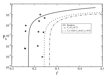
Figure 3: $P_{b}$ (decoder bit error rate) vs. $f$ (channel bit error rate) with rate $R=\frac{1}{3}$ for uncorrelated sequences; for sequences with $C_{1}=C_{2}=0.72$; and for sequences with $C_{1}=-0.65$, $C_{2}=0.6$, $C_{3}=-0.55$ . Results of simulations using KS codesKS-LDPC , with $N=10^{4}$ (9,999 for GF(8)), averaged over at least 2,000 samples, are given for the regular algorithm ($\blacklozenge$) and for the new algorithm ($\blacksquare$ and $\medbullet$ for the 2 and 3 autocorrelations respectively).

Figure 3 shows the results of simulations for uncorrelated messages, and messages with 2 and 3 autocorrelation constraintssimul-y-value . The performance of all 3 cases is similar, both in the number of iterations, and in the distance from their respective limitsperformance ; gzip .

Although we demonstrated the ability to increase the possible noise rate the decoder can handle while keeping the rate fixed, the converse is also possible. Keeping the channel noise fixed, higher rates are achievable. Turning to figure 1, the rate is defined as $R\equiv\frac{K}{N}$, but our encoder compresses the messages as well, thus the achievable rate is actually greater. For $P_{b}=0$, the total rate is $R^{\star}\equiv\frac{L}{N}=\frac{R}{H\left(X\right)}$ (where $H\left(X\right)$ is the entropy of the message); for $H\left(X\right)<R$ rates greater than 1 are feasible.

The complexity of the encoding process remains linear ($O\left(N\right)$), since the calculation of a small number of autocorrelation coefficients is linear. The decoder’s complexity per iteration scales as $\frac{N}{t}q^{2}u$ for a LDPCC decoder over $GF\left(q\right)$, with $\frac{N}{t}$ blocks, and $u$ checks per blockLDPC-GF(q) . Our decoder adds an order of $\frac{N}{t}\left(q^{2}+q\right)$ operations for the calculation of the block prior probabilities, calculating $q$ probabilities, based on the pairs of $q$ states of the 2 neighboring blocks, in equation 13. The algorithm lends itself to parallel implementation which can reduce the complexity to $O\left(1\right)$.

All simulations shown in this paper were done assuming BSC, however the formulation is channel independent, and can be applied to any channel (e.g., the popular Gaussian channel). The method can be also applied to different codes as well (e.g., Turbo-Code), by taking into account the dynamically updated block probabilities.

The method described in this paper can easily be extended to higher order correlation functions (e.g., 3-point correlation function, i.e., $C_{kk\prime}=\frac{1}{L}\sum_{i=1}^{L}X_{i}X_{i+k}X_{i+k\prime}$, with periodic boundary conditions). Adding more correlations has the effect of reducing the entropy by lifting the degeneracy associated with 2-point correlation functions. The size of the transfer-matrix, however, does not have to increase, thus the decoding complexity is unchanged. For example, a transfer matrix of two bits can accommodate 1 additional autocorrelation - $C_{12}$, and a transfer matrix of 3 bits can accommodate 3 additional autocorrelations - $C_{12}$, $C_{13}$, $C_{123}$, the last one being a 4-point correlation functionsymbols .

We have demonstrated the ability to nearly saturate Shannon’s limit without compression mechanisms. The algorithm can be used for utilizing specific noise statistics as well. This work paves the way for additional extensive theoretical research and various practical implementations.

Fruitful discussions with E. Kanter are acknowledged. We would like to thank Shlomo Shamai for critical comments on the manuscript.

References

- (1) C. E. Shannon. A mathematical theory of communication. Bell System Technical J., 27:398-403, 1948
- (2) J. Ziv and A. Lempel. Compression of individual sequences via variable-rate coding. IEEE Trans. Information Theory, IT-24:530-536, 1978
- (3) The reduced autocorrelation coefficients which occur for typical messages (high entropy), are not to be confused with low-autocorrelated sequences which have extremely low entropy. For a recent discussion see: L. Ein-Dor et al., Phys. Rev. E 65, 020102, 2002
- (4) A. Bunde and S.Havlin. Fractals in Science. Springer-Verlag Berlin, 1994
- (5) I. Kanter and D. Kessler. Phys. Rev. Lett.74, 4559, 1995
- (6) M. C. Davey and D. J. C. Mackay. Low Density Parity Check Codes Over GF(q). IEEE Communications Letters, Vol 2, No. 6, June 1998
- (7) Note that instead of (the original binary values). This mapping was introduced by N. Sourlas, Nature 339, 6227, 1989
- (8) R. J. Baxter. Exactly Solved Models In Statistical Mechanics. Academic Press, 1982
- (9) Corrections to the leading order are of the type , see for instance baxter-TM
- (10) The entropy of a single correlation constraint is obtained in a straightforward fashion by performing a gauge. For the gauge gives new variables with a bias , and the entropy is given by Shannon’s result, eq. 1
- (11) Note that imposing short range autocorrelation constraints, , induces long repetitions, symbols, in the sequence. For example, for positive and , one finds subsequences of the same binary digit, whose length is much greater than 2 (the autocorrelation range).
- (12) The sign of each interaction can be positive or negative, leading to frustration. As the entropy approaches the transition, the absolute values of the interactions () diverge.
- (13) S. Y. Chung, G. D. Forney, T. J. Richardson and R. L. Urbanke. On the design of low-density parity-check codes within 0.0045 dB of the Shannon limit. IEEE Commun. Lett. 5 (2). 2001
- (14) T. J. Richardson, M. A. Shokrollahi and R. L. Urbanke. Design of Capacity-Approaching Irregular Low-Density Parity-Check Codes. IEEE Trans. Information Theory, vol. 47, pp. 619-656, 1978
- (15) I. Kanter and D. Saad. Phys. Rev. Lett. 83, 2660, 1999
- (16) The range of and is specified for the MN class of LDPCC, for Gallager-type codes ,
- (17) The interaction strengths for the simulations shown in figure 3 are: (, )/(, , ) for the 2/3 autocorrelation constraints respectively.
- (18) The number of decoder iterations ranges from iterations when the noise level is low, to a few tens of iterations when the threshold of the code is approached. The maximal noise level tolerated by the decoder is within 10% of (the bound for the noise level for infinite length messages) in all 3 cases.
- (19) Given the channel characterization, , the usual method would consist of applying standard compression algorithms (e.g. compress, gzip, bzip2), and then sending the compressed message at the appropriate rate. For the 2 classes shown in figure 3, the measured compression in simulations is about 80% of the entropy (for sequences up to ). Our results are superior in that they utilize the message entropy to a greater extent, as can be seen from figure 3.
- (20) The number of autocorrelation functions grows exponentially with the block size, as do the number of symbols for a given block, which are used in most compression techniques.