Phase transitions in some epidemic models defined on small-world networks

Abstract

Some modified versions of susceptible-infected-recovered-susceptible (SIRS) model are defined on small-world networks. Latency, incubation and variable susceptibility are included, separately. Phase transitions in these models are studied. Then inhomogeneous models are introduced. In some cases, the application of the models to small-world networks is shown to increase the epidemic region.

Keywords: Phase transition; Epidemic models; Small-world networks; Distant-neighbors models; Inhomogeneous models.

1 Introduction

There are many mathematical models for epidemics [1-5]. Generally, the population is classified into susceptible (S), infected (I) and recovered (R) according to the state of each individual. The SIRS model is proposed to describe the outbreaks of foot-and-mouth disease (FMD) [1]. The model is generalized to include latency, incubation and variable susceptibility [4]. They have studied phase transitions in these models. Also it is shown that [5] a ring vaccination programme is capable of eradicating FMD in SIRS model defined on small-world networks (SWN).

The concept of SWN [2,3] is proposed to describe some real social networks. Therefore SWN is used successfully to model several real systems [5-8].

Here our aim is to study phase transitions in some modified versions of SIRS model (including inhomogeneous mixing, latency, incubation and variable susceptibility) defined on SWN.

The paper is organized as follows: In section 2, the concept of SWN is explained. Phase transitions in some SIRS versions are studied in section 3. In section 4, some generalized versions are discussed. Some conclusions are summarized in Section 5.

2 Small-world networks

If one considers all human in the world are occupying the vertices of a network, this social network has to satisfy two main properties: clustering and small-world effect [9]. Clustering means every one has a group of collaborators, some of them will often be a collaborator by another individual. Small-world effect means the average shortest vertex-to-vertex distance, $l$, is very short compared with the size of the network $N$ (the total number of vertices).

Regular lattices display the clustering property, because its clustering coefficient is high. The clustering coefficient $(C)$ is defined as the average fraction of pairs of neighbors of a vertex which are also neighbors of each other. But regular lattices do not display the small-world effect, because the distance $l$ increases as $N^{1/d}$ in $d$ dimensions.

For a random graph [10] with coordination number $z$, the total number of vertices $N$ is given by

$$N=z^{l},$$

which gives,

$$l=\frac{\log\,N}{\log\,z}.$$ (1)

The logarithmic increase with $N$ allows the distance $l$ to be very short even for large $N$. Then random graphs display the small-world effect. But a random graph does not satisfy the clustering property, because its clustering coefficient is given by $C=z/N,\,$ this quantity goes to zero for large $N$. Therefore both regular and random lattices are not good descriptions for social networks.

A SWN consists of a regular one-dimensional (1-d) chain with periodic boundary conditions. Each vertex is connected to its nearest-neighbors by bonds. Some shortcutting bonds joining between some randomly chosen vertices with probability $\phi$ are added. The probability $\phi$ is supposed to be small in order to preserve the clustering property of the regular lattice. The small-world effect is concluded as follows: for very small lattice size $N$, it is less probable to find a shortcut, so the system behaves like a regular lattice, and

$$l\propto N.$$ (2)

When $N$ becomes large enough, more shortcuts are expected and the system behaves as a random lattice i.e.

$$l\propto\log\,N.$$ (3)

Consider this transition occurs at certain system size $\zeta$, then $l$ obeys a finite size scaling law as

$$l=Nf\left(\frac{N}{\zeta}\right),$$

where $f(x)$ is a universal scaling function, such that

$$f(x)=\left\{\begin{array}[]{c}{\rm{const.}}\;\;\;{\rm{if}}\;x\ll 1,\\ \frac{\log x}{x}\;\;\;\;\;\;{\rm{if}}\;x\gg 1.\end{array}\right.$$ (4)

After some calculation using the renormalization group theory [9], one gets

$$l=Nf(\phi N),$$

for 1-d and considering the first-nearest neighbors only ($d=1$, $k=1$), and

$$l=\frac{N}{k}f((\phi k)^{\frac{1}{d}}N),$$ (5)

for general $k$-distance-nearest neighbors and any $d$. These forms are valid only for $N\gg 1$ and $\phi\ll 1$. Then for $N\gg 1/\phi$,

$$l\propto\log N.$$

Then SWN are shown to combine both properties of social networks. Also this structure combines between both local and non local interactions which is observed in many real systems. Therefore the concept of SWN is used in modelling several real systems [5-8]. Here our interest is restricted to apply the concept of SWN to some epidemic models.

3 Phase transitions in some epidemic models

The population is classified into three classes: susceptible, infected and recovered. Consider a function $s(i,t)$ represents the state of an individual $i$ at time $t$, such that,

$$s(i,t)=\left\{\begin{array}[]{l}-1\;\;\;{\rm{for\;I-individuals,}}\\ 0\;\;\;\;\;\;{\rm{for\;S-individuals,}}\\ 1\;\;\;\;\;\;{\rm{for\;R-individuals.}}\end{array}\right.$$

The transitions between the states S, I and R occur according to the following automata rules:

1. Infection:

   If $s(i,t)=0$ and ($s(i-1,t);s(i+1,t)$ or both $=-1$), then $s(i,t+1)=-1$ with probability $p_{1}$.

2. Recovery:

   $${\rm{If}}\;s(i,t)=-1,\;{\rm{then}}\;s(i,t+1)=1.$$ (6)

3. Losing immunity:

   $${\rm{If}}\;s(i,t)=1,\;{\rm{then}}\;s(i,t+1)=0\;{\rm{with\;probability}}\;p_{2}.$$ (7)

This model is approximated by the following set of differential equations:

$$\frac{{\rm{d}}S}{{\rm{d}}t}=p_{2}R-p_{1}SI,$$ (8)

$$\frac{{\rm{d}}I}{{\rm{d}}t}=p_{1}SI-I,$$ (9)

$$\frac{{\rm{d}}R}{{\rm{d}}t}=I-p_{2}R$$ (10)

This set of differential equations is a mean field approximation that ignores the spatial structure of the lattice. It assumes a global interacting system. But in reality a disease spreads locally with some non local interactions. Also including some epidemic aspects like lower susceptibility, incubation to the differential equations is very difficult. On the other hand, it is allowed in lattice models [4,5].

To study the phase transition in this model, the probabilities $p_{1}$ and $p_{2}$ are varied from $0$ to $1$ by step $0.01$. The phase diagram is drawn as a relation between $p_{1}$ and $p_{2}$. There are two limiting points: The first is when $p_{2}=0$ corresponding to the case of perfect immunization, and it is close to ordinary percolation [11]. The second case is for $p_{2}=1$ representing the case of zero immunization, and this case is well described by directed percolation [12]. For intermediate values of $p_{2}$, there are no clear relation to the percolation theory. The phase diagram is similar to damage spreading transitions [13], where two phases appear: epidemic and non epidemic.

Ahmed and Agiza [4] have studied phase transitions in some modified versions of 1-d SIRS model including inhomogeneous mixing, latency, incubation and variable susceptibility. Here we will generalize their work to SWN. The SWN used here is a 1-d chain of size $1000$ with periodic boundary conditions. Shortcuts are fixed beforehand with probability $\phi=0.05$ per bond. The models evolve for $10000$ time steps. We will study four different versions of SIRS model separately.

The first is the original SIRS itself. The automata rules are generalized to include the shortcutting neighbors as follows:

1. Infection: If $s(i,t)=0$ and $(s(i-1,t);\;s(i+1,t)$ or $s(s_{c}(i),t)$ (if exists), at least $=-1$), then $s(i,t+1)=-1$ with probability $p_{1},$ where $s_{c}(i)$ is the shortcutting neighbor of the $i$-th individual (if exists).

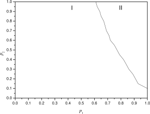
Figure 1: Phase diagram for the SIRS model defined on SWN with $N=1000$, $\phi=0.05$ and $k=1$. Tow phases appear nonepidemic (I) and epidemic (II), and $p_{1c}=0.61$.

Rules for both recovery and losing immunity are the same as the original model. The phase diagram is shown in Fig. 1. It appears that an epidemic phase occurs at $p_{1c}=0.61$. This value is slightly less than that observed from the 1-d original model.

In some cases, an infection does not spread directly, but it needs some time and suitable conditions to be transmitted. In order to model this phenomenon, the population is classified into four states: susceptible, infected, recovered and lower susceptible. Then the state function is modified to:

$$s(i,t)=\left\{\begin{array}[]{l}-1\;\;\;{\rm{for\;I-individuals,}}\\ 0\;\;\;\;\;\;{\rm{for\;S-individuals,}}\\ 0.5\;\;\;{\rm{for\;lower\;susceptible\;individuals,}}\\ 1\;\;\;\;\;\;{\rm{for\;R-individuals.}}\end{array}\right.$$ (11)

A lower susceptible individual has immunity greater than a susceptible individual; but smaller than a recovered one. The model is defined on SWN. Consider $30\%$ of the population have a lower susceptibility. Both infection and recovery rules are the same as in the first case. The other rules are modified to:

1. Losing immunity: if $s(i,t)=1$, then with probability $p_{2},$

   $$s(i,t+1)=\left\{\begin{array}[]{l}0\;\;\;\;\;{\rm{with\;probability}}\;0.7,\\ 0.5\;\;\;{\rm{with\;probability}}\;0.3.\end{array}\right.$$ (12)

2. Susceptibility:

   If $s(i,t)=0.5$ and $(s(i-1,t);s(i+1,t)$ or $s(s_{c}(i),t)$ (if exists), at least $=-1$), then $s(i,t+1)=0$.

The phase diagram is given in Fig. 2. The epidemic phase occurs at $p_{1c}=0.71$. The epidemic region is smaller than that of the first case, because of the assumption that $30\%$ of the population are not infected directly.

The third case, in some infectious diseases, a diseased individual can be infecting but symptoms don’t appear (incubation state). On the other hand, an infected individual may not be infecting but still has the symptoms (i.e. latent state). This case is called incubation-latent model. We define this model on SWN as follows: The state function is modified to:

$$s(i,t)=\left\{\begin{array}[]{l}-2\;\;\;{\rm{represents\;incubation,}}\\ 0\;\;\;\;\;\;{\rm{represents\;susceptibility,}}\\ 1\;\;\;\;\;\;{\rm{represents\;recovery,}}\\ 2\;\;\;\;\;\;{\rm{represents\;latency.}}\end{array}\right.$$ (13)

The rule of losing immunity is the same as in the original model; but the other rules are modified as follows:

1. Incubation:

   If $s(i,t)=0$ and ($s(i-1,t);s(i+1,t)$ or $s(s_{c}(i),t)$ (if exists), at least $=-2$), then $s(i,t+1)=-2$ with probability $p_{1}$.

2. Recovery:

   If $s(i,t)=2$, then $s(i,t+1)=1$.

3. Latency:

   If $s(i,t)=-2$, then $s(i,t+1)=2$.

The results are shown in Fig. 3, the epidemic region extended again with $p_{1c}=0.61$. This case is similar but not identical to first case.

Fourth, an incubation both sick and infecting model is introduced. In some diseases like Aids, a diseased person is sick and infecting, so this model is called an incubation both sick and infecting model. The state function $s(i,t)$ is defined as follows:

$$s(i,t)=\left\{\begin{array}[]{l}-2\;\;\;{\rm{represents\;incubation,}}\\ -1\;\;\;{\rm{represents\;sick\;and\;infecting,}}\\ 0\;\;\;\;\;\;{\rm{represents\;susceptibility,}}\\ 1\;\;\;\;\;\;{\rm{represents\;recovery.}}\end{array}\right.$$ (14)

The model is defined on SWN, and the automata rules become:

1. Incubation:

   If $s(i,t)=0$ and $(s(i-1,t)<0$; $s(i+1,t)<0$ or $s(s_{c}(i),t)<0$ (if exists), at least), then $s(i,t+1)=-2$ with probability $p_{1}$.

2. Sick-Infected:

   If $s(i,t)=-2$, then $s(i,t+1)=-1$.

Rules for both recovery and losing immunity are the same as in the original model. The phase diagram is shown in Fig. 4, the epidemic phase occurs at $p_{1c}=0.41$. The epidemic region is extended more than the previous cases, because infection is expected from both sick-infected and incubation individuals.

4 Some generalizations

Sometimes an infection is transmitted to some distant neighbors in addition to the nearest neighbors. This interaction with the distant neighbors is modelled by generalizing the automata rules, discussed in the previous section, to include distant neighbors at a distance $k$. This means $k=1$ gives the first-nearest neighbors, $k=2$ gives the second-nearest neighbors in addition to the first-nearest neighbors, and so on. The case $k=2$ is studied for the four cases, and the results are summarized in table 1. The epidemic phase increased significantly in the four cases. This is expected, because the infection spreads faster than in the case of $k=1$.

Generally, every individual has his/her own immune system that differs significantly from the others. Thus the susceptibility also differs from one to another. Also, in some cases the probability of infection depends on the number of infected neighbors. To model this behavior, a modified probability of infection is considered. If $p_{1}$ is the probability of infection due to one infected nearest neighbor, then $(1-$ $p_{1})^{m}$ is the probability of noninfection due to $m$ infected nearest neighbors. Then the modified probability of infection [14] is

$$p_{1}^{*}=1-(1-p_{1})^{m},$$ (15)

per unit of time. Beside the advantages of this form, it also implies that the probability of infection for each individual is not constant with time. Using $p_{1}^{*}$ instead of $p_{1}$ is introducing inhomogeneity that is one of the main aspects in reality.

Inhomogeneous models are constructed for the four cases studied in the previous section. The same conditions are applied. The results are close to that of the models in SWN, but there are slight differences from the results of the 1-d models. A comparison between the results of regular lattice, SWN with $k=1$, SWN with $k=2$ and the inhomogeneous models is given in Table 1.

$p_{1c}$	Regular lattice $k=1$ [4]	SWN $k=1$	SWN $k=2$	Inhomogeneous Models
Case 1	0.68	0.61	0.38	0.60
Case 2	0.80	0.71	0.43	0.74
Case 3	0.67	0.61	0.40	0.59
Case 4	0.47	0.41	0.24	0.40

Table 1: The critical value $p_{1c}$ at which the phase transition occurs for all the studied models.

5 Conclusions

Phase transitions in some modified versions of SIRS model for epidemics are studied using SWN with both $k=1$ and $k=2$. Also, inhomogeneous models are introduced. Only the case of $k=2$ is found to significantly affect the phase transitions in all models. Just slight changes are found in the other cases.

Acknowledgements

We thank E. Ahmed for helpful discussions.

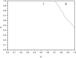
Figure 2: Phase diagram for the SIRS model defined on SWN with $N=1000$, $\phi=0.05$ and $k=1$. Lower susceptibility is introduced. The critical value is $p_{1c}=0.71$.

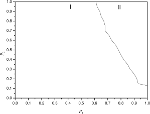
Figure 3: Phase diagram for the third case, where an incubation-latent model is defined on SWN with $N=1000$, $\phi=0.05$ and $k=1$. The phase transition occurs at $p_{1c}=0.61$.

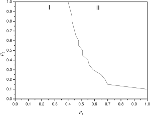
Figure 4: Phase diagram for a modified version of SIRS model including the concept of incubation both sick and infecting. The model is defined on SWN with $N=1000$, $\phi=0.05$ and $k=1$. A phase transition from nonepidemic to epidemic phases is observed at $p_{1c}=0.41$.

References

- [1] L. Edelstein-Keshet, ”Mathematical Models in Biology”, (Random House, New York, 1988).
- [2] M. E. J. Newman and D. J. Watts, Phys. Rev. E 60, 7332 (1999).
- [3] C. Moore and M. E. J. Newman, cond-mat/9911492v2 (1999).
- [4] E. Ahmed and H. N. Agiza, Physica A 253, 347 (1997).
- [5] E. Ahmed, A. S. Hegazi and A. S. Elgazzar, Int. J. Mod. Phys. C 13, 189 (2002).
- [6] E. Ahmed and A. S. Elgazzar, Europ. Phys. J. B 18, 159 (2000).
- [7] A. S. Elgazzar, Int. J. Mod. Phys. C 12, 1537 (2001).
- [8] A. S. Elgazzar, Physica A 303, 154 (2002).
- [9] M. E. J. Newman and D. J. Watts, Phys. Lett. A 263, 341 (1999).
- [10] B. Bollobas, ”Random Graphs”, (Academic Press, New York, 1985).
- [11] A. Aharony and D. Stauffer, ”Introduction to Percolation Theory”, (Taylor and Francis, London, 1992).
- [12] P. Grassberger, Univ. Wuppertal Preprint, (1995).
- [13] P. Grassberger, J. Stat. Phys. 97, 13 (1995).
- [14] C. B. dos Santos, D. Barbin and A. Caliri, Phys. Lett. A 238, 54 (1998).