In Search of the Vortex Loop Blowout Transition
for a type-II Superconductor in a Finite Magnetic Field

Abstract

The 3D uniformly frustrated XY model is simulated to search for a predicted “vortex loop blowout” transition within the vortex line liquid phase of a strongly type-II superconductor in an applied magnetic field. Results are shown to strongly depend on the precise scheme used to trace out vortex line paths. While we find evidence for a transverse vortex path percolation transition, no signal of this transition is found in the specific heat.

I Introduction

In pure extreme type-II superconductors, such as the high $T_{c}$ superconductors, the Abrikosov vortex line lattice melts via a sharp first order phase transitionR1 into a vortex line liquid as the temperature is increased above a critical $T_{m}$. The properties of this vortex line liquid phase have been the subject of considerable investigation. Theoretical argumentsR2 and early simulationsR3 ; R3.1 ; R3.2 suggested that the vortex line liquid might retain superconducting phase coherence parallel to the applied magnetic field, within some temperature interval above $T_{m}$. Later, better converged simulationsR4 found that phase coherence is simultaneously lost in all directions upon melting.

Subsequently, TešanovićR5 has proposed that, for small magnetic fields, there still remains a sharp thermodynamic phase transition at a temperature $T_{\Phi}$ within the vortex liquid state, associated with diverging fluctuations of closed vortex loops, such as drive the superconducting transition in the zero magnetic field case. Considering the limit of infinite penetration length $\lambda$, Tešanović proposed that, in a finite field, the fluctuations of the magnetic field induced vortex lines act to screen the interactions of thermally excited closed vortex loops, in the same way that magnetic field fluctuations screen the vortex loop interactions of a finite $\lambda$ model in zero applied magnetic field. Pursuing this argument, he predicted that the proposed vortex loop blowout transition at $T_{\Phi}$ may be an inverted XY transition, as is the case of the zero field Meissner transition for the finite $\lambda$ model.

Following Tešanović’s predictions, Sudbø and co-workersR6 ; R7 ; R8 have carried out numerical simulations of the three dimensional (3D) uniformly frustrated XY model of a type-II superconductor. They claim to find evidence for Tešanović’s transition, which they associate with the formation of a vortex line path that percolates entirely around the system in the direction transverse to the magnetic field.

Most recently, measurementsR9 on high purity YBa₂Cu₃O₇ (YBCO) single crystals have found a step like anomaly in the specific heat at a temperature highter than the melting $T_{m}$, reminiscent of an inverted mean field transition. It has been arguedR9 that this feature may be evidence for Tešanović’s transition $T_{\Phi}$.

In order to further investigate this issue, we have carried out new simulations on the 3D uniformly frustrated XY model, both repeating the approach of Sudbø and co-workers, and measuring new quantities that make a more direct test of Tešanović’s theory. After correcting certain inconsistencies in the earlier numerical work, we show that whether or not one finds indications of a vortex loop blowout transition depends crucially on how one chooses to resolve vortex line paths at points where two or more lines intersect. Making the choice that favors the blowout interpretation, we find the critical exponent $\nu\simeq 1$, rather than the value $\sim 2/3$ expected for an inverted 3D XY transition. Finally, we make high precision measurements of the specific heat, in search of a thermodynamic signature for a blowout transition, but no such signature is found.

II Model

The model that we use is the 3D uniformly frustrated XY modelR3 ; R3.1 ; R3.2 ; R4 ; R6 ; R7 ; R8 ; R10 which models a type-II superconductor in the limit of infinite magnetic penetration length, $\lambda\to\infty$, and is given by the Hamiltonian,

$${\cal H}[\theta_{i}]=-\sum_{i,\mu}J_{\mu}\cos(\theta_{i+\hat{\mu}}-\theta_{i}-A_{i\mu})\enspace.$$ (1)

Here $i$ are the nodes of a cubic grid of sites, $\mu=x,y,$ $z$, are the directions of the grid axes, and the sum is over all nearest neighbor bonds of the grid. $\theta_{i}$ is the phase angle of the superconducting wavefunction on site $i$, $A_{i\mu}=(2\pi/\Phi_{0})\int_{i}^{i+\hat{\mu}}{\bf A}\cdot d{\bf r}$ is given by the integral of the magnetic vector potential ${\bf A}$ across the bond at site $i$ in direction $\hat{\mu}$, and $\Phi_{0}=hc/2e$ is the flux quantum. The argument of the cosine is the gauge invariant phase angle difference across the bond. The circulation of the $A_{i\mu}$ around any plaquette of the grid is equal to $2\pi$ times number of flux quanta of magnetic field penetrating the plaquette. We take the magnetic field, ${\bf B}=\nabla\times{\bf A}$, uniform and parallel to the $\hat{z}$ axis, with a fixed density of flux quanta $f=Ba^{2}/\Phi_{0}$ per plaquette of area $a^{2}$. The couplings $J_{\mu}$ we take to model an anisotropic system, with $J_{x}=J_{y}\equiv J_{\perp}$, and $J_{z}\leq J_{\perp}$.

Simulations are carried out varying the $\theta_{i}$ according to a usual Monte Carlo scheme; the $A_{i\mu}$ are held fixed. That the $A_{i\mu}$ do not fluctuate, and that they give a uniform magnetic field, are the consequences of the $\lambda\to\infty$ approximation. Simulations are carried out on $L_{z}\times L_{\perp}^{2}$ cubic grids, using periodic boundary conditions. Except where otherwise noted, our runs are typically for $1/4$ to $1/2\times 10^{6}$ Monte Carlo passes through the entire lattice.

While we simulate in the phase angle degrees of freedom, $\theta_{i}$, our interest will be in the behavior of the vorticity in these phase angles. Let $s$ denote the dual sites of the original grid; these are the sites at the centers of the unit cells of the grid. Denote by $(s,\mu)$ the plaquette which is the face of the unit cell centered on dual site $s$ with normal in the $\hat{\mu}$ direction, $\mu=x,y$, $z$. We define the integer vorticity $n_{s\mu}$ piercing plaquette $(s,\mu)$ by computing the circulation of the gauge invariant phase angle differences around the plaquette,

$$\sum_{(s,\mu)}[\theta_{i+\hat{\sigma}}-\theta_{i}-A_{i\sigma}]=2\pi(n_{s\mu}-f\delta_{z\mu})\enspace,$$ (2)

where the sum is counterclockwise around all bonds forming the boundary of plaquette $(s,\mu)$, and the gauge invariant phase angle differences are restricted to the interval $[-\pi,\pi)$. In a constant magnetic field, the condition that the total energy density remains finite can be shown to yield the “neutrality” constraint (see section III.A),

$$\sum_{s}n_{s\mu}=fL_{\perp}^{2}L_{z}\delta_{z\mu}\enspace,$$ (3)

i.e. the total vorticity piercing any plane at constant $z$ is $fL_{\perp}^{2}$; these are the magnetic field induced vortex lines. The total vorticity in the transverse directions $x$ and $y$ is zero.

Taking the vorticity $n_{s\mu}$ as the directed bond of the dual grid, emanating from site $s$ in direction $\hat{\mu}$, the vorticity so defined is divergenceless, forming continuous lines that, due to the periodic boundary conditions, must ultimately close upon themselves. We will label such a closed vortex path by the index $\alpha$, and define the vector ${\bf R}_{\alpha}$ as the net displacement one travels upon following the path $\alpha$ from a given starting point until returning back to that point as the line closes back on itself. If ${\bf R}_{\alpha}=0$, then the vortex line path is a closed loop of finite extent that exists as a thermal fluctuation. If $R_{z\alpha}=mL_{z}$, $m$ integer, then such a vortex line path represents $m$ of the $fL_{\perp}^{2}$ field induced vortex lines; these $m$ lines are mutually connected to each other via the periodic boundary conditions in the $z$ direction.R3.1 For $m>1$, we can say that the $m$ field induced lines are geometrically entangled with each other. If $R_{x\alpha}=mL_{\perp}$ or $R_{y\alpha}=mL_{\perp}$, then the vortex line path winds $m$ times around the system transversely to the applied magnetic field. We will be particularly interested in vortex line paths for which $R_{z\alpha}=0$, but $R_{x\alpha}$ or $R_{y\alpha}\neq 0$. Henceforth, we will refer to as the “lines”, the set of vortex line paths $\{\alpha\}$ for which all $R_{z\alpha}>0$; these are the field induced vortex lines. All other vortex paths we will refer to as the “loops”.

In order to trace out vortex line paths, one needs to know how to treat intersections. An intersection is when there is more than one vortex line entering and exiting a give unit cell of the grid, and it is therefore ambiguous which entering segment to connect to which exiting segment. It was previously shownR11 by one of us that the method chosen to resolve such intersections can have a dramatic effect on the statistics of closed thermally excited loops in the zero field $f=0$ model. Here, for the $f>0$ model, we consider two different schemes, which we henceforth refer to as method (i) and method (ii):

(i) At each intersection we choose randomly, with equal probability, which entering segment connects to which exiting segment. In the $f=0$ model this scheme was found to give results closest to theoretical expectations.R11

(ii) Motivated by Sudbø and co-workers,R6 ; R7 ; R8 we first searchR11.1 through all possible connections to find a path $\alpha$ with $R_{z\alpha}=0$ and $R_{x\alpha}$ or $R_{y\alpha}\neq 0$. Such a path winds around the system transverse to the field, without ever winding around the system parallel to the field. If one such path is found, it is selected as a path $\alpha^{\prime}$ contributing to the “loops”, and we then repeat the proceedure applied to all remaining vortex paths. When all such transverse paths are found, the remaining vortex line intersections are resolved randomly, as in method (i).

Using either method (i) or method (ii) we thus decompose the vorticity of any given configuration into disjoint closed vortex line paths, consisting of a set $\{\alpha\}$ of “lines” and a set $\{\alpha^{\prime}\}$ of “loops”.

III Winding of Field Induced Vortex Lines

We first attempt a direct test of Tešanović’s theory of the $T_{\Phi}$ transition within the liquid phase. A summary of his arguments for the existence of this transition is as follows.

III.1 Summary of Tešanović’s Theory

First, a duality transformationR12 ; R12.1 ; R12.2 from the XY model of Eq. (1) gives the interaction between vortices as,

$${\cal H}[n_{s\mu}]={1\over 2}\sum_{s,s^{\prime},\mu}[n_{s\mu}-f\delta_{z\mu}]V^{\mu}({\bf r}_{s}-{\bf r}_{s^{\prime}})[n_{s^{\prime}\mu}-f\delta_{z\mu}]$$ (4)

where $V^{\mu}({\bf r})$ is the appropriate anisotropic generalization of the Coulomb interaction, with Fourier transform $V_{q}^{\mu}\sim q^{-2}$. It is this singularity of $V_{q}^{\mu}$ as $q\to 0$ that yields the constraint of Eq. (3).

Next, one imagines decomposing the total vorticity of the system into lines and loops,

$$n_{s\mu}=n_{s\mu}^{\mathrm{lines}}+n_{s\mu}^{\mathrm{loops}}\enspace.$$ (5)

If we define,

$$b_{s\mu}\equiv n_{s\mu}^{\mathrm{lines}}-f\delta_{z\mu}$$ (6)

then $\sum_{s}\langle b_{s\mu}\rangle=0$ and the Hamiltonian of Eq. (4) can be rewritten as,

$${\cal H}={1\over 2}\sum_{s,s^{\prime},\mu}[n_{s\mu}^{\mathrm{loops}}-b_{s\mu}]V^{\mu}({\bf r}_{s}-{\bf r}_{s^{\prime}})[n_{s^{\prime}\mu}^{\mathrm{loops}}-b_{s^{\prime}\mu}]\enspace.$$ (7)

Tešanović then argues that a coarse graining of vortex fluctuations, in the vortex line liquid phase, leads to an effective hydrodynamic Hamiltonian on long length scales which has the same interaction piece as Eq. (7), but which has a new additive term proportional to $\sum_{s\mu}b_{s\mu}^{2}$. The resulting long length scale Hamiltonian then has exactly the same form as that of a zero field superconductor with thermally fluctuating vortex loops, $n_{s\mu}^{\mathrm{loops}}$, and a thermally fluctuating magnetic field $b_{s\mu}$ whose average is zero, i.e. the zero field superconductor with a finite penetration length $\lambda$. In other words, in this infinite $\lambda$ theory at finite magnetic field, the long wave length fluctuations of the field induced vortex lines $n_{s\mu}^{\mathrm{lines}}$ screen the interaction between the vortex loops $n_{s\mu}^{\mathrm{loops}}$ in exactly the same manner as magnetic field fluctuations screen the interactions between vortex loops in a finite $\lambda$ model at zero magnetic field.

The Meissner transition at $T_{c}$ in the zero field, finite $\lambda$, model is an inverted 3D XY transition.R12 The high temperature phase $T>T_{c}$ has vortex loops on all length scales and breaks a global $U(1)$ symmetry associated with a disorder parameter;R12.3 the low temperature phase $T<T_{c}$ has no vortex loops on sufficiently long length scales. The correlation length $\xi$ and renormalized magnetic penetration length $\lambda_{R}$ both divergeR13 as $\sim|t|^{-\nu}$, with $\nu\simeq 2/3$ and $t\equiv T-T_{c}$.

We have earlier carried out numerical simulationsR13 of this zero field, finite $\lambda$, Meissner transition. We demonstrated that, in this model, magnetic field fluctuations obey the finite size scaling relation,

$$F(t,q,L) \equiv \langle b_{\mu}(q\hat{\nu})b_{\mu}(-q\hat{\nu})\rangle/L^{3}$$ (8)

$$\sim L^{-1}F(tL^{1/\nu},qL,1)$$

where in the above $\hat{\mu}\perp\hat{\nu}$ and $b_{\mu}(q\hat{\nu})=\sum_{s}e^{-iq\hat{\nu}\cdot{\bf r}_{s}}b_{s\mu}$ is the Fourier transform of of the magnetic flux density $b_{s\mu}$. As $L\to\infty$, and $q\to 0$,

$$F(t,0,\infty)\sim\left\{\begin{array}[]{ll}0&t<0\\ 1/\xi&t>0\end{array}\right.\enspace,$$ (9)

hence $F(t,0,\infty)$ vanishes below the transition, and increases continuously from zero as one goes above the transition.

In the present case of a finite magnetic field, if Tešanović’s mapping is correct, the Meissner transition $T_{c}$ becomes the transition $T_{\Phi}$ within the vortex line liquid phase, and we expect the exact same scaling as in Eq. (8) above, when applied to the quantity $b_{s\mu}$ defined in Eq. (6). Taking the limit of $q\to 0$ in Eq. (8), and applying to systems with fixed aspect ratio $L_{z}=gL_{\perp}$, we expect the scaling,

$$\big{\langle}(\sum_{s}b_{s\mu})^{2}\big{\rangle}/L_{\perp}^{3}\sim L_{\perp}^{-1}f(tL_{\perp}^{1/\nu})\enspace,$$ (10)

where $t\equiv T-T_{\Phi}$ and $f(x)=F(x,0,1)$.

For the directions $\hat{\mu}=\hat{x}$ or $\hat{y}$,

$$\sum_{s}b_{s\mu}=\sum_{s}n_{s\mu}^{\mathrm{lines}}\equiv W_{\mu}L_{\perp}$$ (11)

is the net vorticity of the magnetic field induced vortex lines in the transverse direction $\hat{\mu}$. The two dimensional vector ${\bf W}=(W_{x},W_{y})$ defined above is the integer valued “winding number” that counts the net number of times the field induced vortex lines wind around the system in the transverse directions $\hat{x}$ and $\hat{y}$. If $\{\alpha\}$ is the set of vortex line paths that define the field induced vortex lines $n_{s\mu}^{\mathrm{lines}}$, and ${\bf R}_{\alpha}$ is the net displacement along path $\alpha$ as defined earlier, then $\sum_{\alpha}{\bf R}_{\alpha\perp}={\bf W}L_{\perp}$, where ${\bf R}_{\perp}\equiv(R_{x},R_{y})$. We thus expect from Eq. (10) the finite size scaling,

$$\langle W^{2}\rangle\sim f(tL_{\perp}^{1/\nu})\enspace.$$ (12)

Note, the neutrality condition of Eq. (3) implies that the total transverse vorticity in the system must always vanish. For ${\bf W}\neq 0$, it is therefore necessary that any such winding of the field induced lines is exactly canceled out by an equal and opposite transverse winding of the loops. In the thermodynamic limit, $L_{\perp}\to\infty$, Eq. (9) implies that $\langle W^{2}\rangle=0$ for $T<T_{\Phi}$, and $\langle W^{2}\rangle$ increases continuously from zero as one increases $T>T_{\Phi}$. The proposed transition at $T_{\Phi}$ is thus associated with the appearance of infinite transverse loops (see following Section IV).

Another interpretation of the $T_{\Phi}$ transition follows from the “two dimensional (2D) boson” modelR14 of interacting vortex lines, in which the field induced vortex lines are viewed as the world lines of two dimensional bosons traveling down the imaginary time axis. For $T<T_{\Phi}$ where $\langle W^{2}\rangle=0$, the field induced vortex lines behave like charged two dimensional bosons,R2 ; R12.2 with a long range retarded Coulomb interaction. In the vortex line liquid, $T_{m}<T<T_{\Phi}$, where phase coherence is lost parallel to the applied magnetic field, the analog 2D bosons are in a charged superfluid state. For $T>T_{\Phi}$, where $\langle W^{2}\rangle\neq 0$, screening by the infinitely large loops $n_{s\mu}^{\mathrm{loops}}$ results in an effective short ranged interaction between the field induced lines. In this case the winding number squared $\langle W^{2}\rangle$ is proportional to the superfluid density of what is now an uncharged superfluid. Thus $T_{\Phi}$ corresponds to a transition between a charged superfluid and an uncharged superfluid in the analog 2D boson theory. Equivalently, if one considers the quanta that mediate the interaction between the analog 2D bosons, the transition is from massless quanta for $T<T_{\Phi}$ to massive quanta for $T>T_{\Phi}$.

To arrive at Eq. (12), we considered the transverse components of Eq. (10). However, we can also consider the parallel, $\hat{\mu}=\hat{z}$ component. Now,

$$\sum_{s}b_{sz}=\sum_{s}n_{sz}^{\mathrm{lines}}-fL_{\perp}^{2}L_{z}\equiv W_{z}L_{z}\enspace,$$ (13)

and so we expect the scaling

$$\langle W_{z}^{2}\rangle\sim f_{z}(tL_{\perp}^{1/\nu})\enspace.$$ (14)

If $\{\alpha\}$ is the set of vortex line paths that define the field induced vortex lines $n_{s\mu}^{\mathrm{lines}}$, and ${\bf R}_{\alpha}$ is the net displacement along path $\alpha$ as defined earlier, then $\sum_{\alpha}R_{\alpha z}=(fL_{\perp}^{2}+W_{z})L_{z}$. Thus $W_{z}$ gives the number of “lines” in excess of the average value $fL_{\perp}^{2}$ set by the applied magnetic field. The neutrality condition of Eq. (3) requires that when $W_{z}>0$, there must be an equal and opposite parallel winding of the loops $n_{s\mu}^{\mathrm{loops}}$. As $L\to\infty$, we have $W_{z}=0$ for $T<T_{\Phi}$, and $W_{z}>0$ for $T>T_{\Phi}$. Thus a transition at $T_{\Phi}$ should be characterized by fluctuations in the number of field induced lines and by the appearance of infinite parallel loops directed opposite to the direction of the applied magnetic field.

III.2 Numerical Results

To test the above predictions, we have simulated the 3D uniformly frustrated XY model of Eq. (1) using a vortex density $f=1/20$, anisotropy $J_{z}/J_{\perp}=0.02$, and aspect ratio $L_{z}/L_{\perp}=1$, for $L_{\perp}=10,$ $20$, $30$, $40$ and $60$. For these parameters, the vortex lattice melting temperature is $T_{m}\simeq 0.24J_{\perp}$, and the zero field critical temperature is $T_{c0}\simeq 1.14J_{\perp}$. We compute the transverse winding ${\bf W}$ of the field induced lines, defined by Eq. (11), using both method (i) and method (ii) to decompose each configuration into “lines” and “loops”. According to the scaling equation (12), we expect that plots of $\langle W^{2}\rangle$ vs. $T$ for different sizes $L_{\perp}$ should all intersect at the common point $t=0$, or $T=T_{\Phi}$.

In Fig. 1 we show a semilog plot of $\langle W^{2}\rangle$ vs. $T/J_{\perp}$ using method (i) (random reconnections at intersections) for $L_{\perp}=10$, $20$, and $30$. We see that there is clearly no common intersection point of the curves. As $L_{\perp}$ increases, $\langle W^{2}\rangle$ decreases uniformly over the entire temperature range. This is in qualitative agreement with earlier computations of $\langle W^{2}\rangle$ by one of us (see Fig. 15 of Ref.R3.1, ). For $L_{\perp}=60$, we have found no net transverse winding of the field induced lines at all, i.e. for the length of our simulation we had ${\bf W}=0$, for the temperature range $1.36\leq T/J_{\perp}\leq 1.44$.

Figure 1: Semilog plot of winding $\langle W^{2}\rangle$ vs. $T/J_{\perp}$ for $L_{\perp}=10$, $20$, and $30$, with vortex density $f=1/20$, anisotropy $J_{z}=0.02J_{\perp}$, and aspect ratio $L_{z}=L_{\perp}$. $\langle W^{2}\rangle$ is computed using method (i), i.e. random connections at intersections. $\langle W^{2}\rangle$ steadily decreases as $L_{\perp}$ increases, over the entire temperature range.

Next, in Fig. 2, we show the same quantities but now using method (ii) (search first for maximal transverse loops), for $L_{\perp}=10,$ $20$, $30$, $40$ and $60$. We see that as $L_{\perp}$ increases, the curves do seem to approach a common intersection point, giving a $T_{\Phi}\simeq 1.4J_{\perp}$. Note that this $T_{\Phi}$ is above the zero field critical temperature $T_{c0}\simeq 1.14J_{\perp}$.

From Eq. (12), we expect that the slopes of these curves at $T_{\Phi}$ should scale with system size as, $d\langle W^{2}\rangle/dT\sim L_{\perp}^{1/\nu}$. Fitting each of the curves of $\langle W^{2}\rangle$ to a cubic polynomial in $T$, we compute their derivatives at the intersection point $T=1.4J_{\perp}$, and plot the results vs. $L_{\perp}$ in Fig. 3. We see that the slopes, to an excellent approximation, scale linearly with $L_{\perp}$, thus suggesting a critical exponent $\nu\simeq 1$. On closer inspection, the data in Fig. 3 show a small systematic downwards curvature about the linear fit; however this curvature can be removed by assuming a slightly higher critical temperature of $T=1.403J_{\perp}$. Note that this value of $\nu\simeq 1$ is larger than the predicted value of $2/3$.

As an alternative method to compute the critical behavior, we can take the scaling equation (12), expand the scaling function $f(x)$ as a polynomial for small $x$, and do a nonlinear fitting to the data to determine the unknown polynomial coefficients, $T_{\Phi}$, and $\nu$. To obtain the best fit we use a 4th order polynomial and fit only the data from the two largest sizes, $L_{\perp}=40$ and $60$. The results give $T_{\Phi}\simeq 1.403J_{\perp}$ and $\nu\simeq 0.96$, in agreement with the earlier estimates. In Fig. 4 we show the scaling collapse that results from this polynomial fit. There are systematic deviations from the fitted curve on the $T>T_{\Phi}$ side, though these appear to decrease as $L_{\perp}$ increases.

Figure 2: Plot of winding $\langle W^{2}\rangle$ vs. $T/J_{\perp}$ for $L_{\perp}=10$, $20$, $30$, $40$, and $60$, with vortex density $f=1/20$, anisotropy $J_{z}=0.02J_{\perp}$, and aspect ratio $L_{z}=L_{\perp}$. $\langle W^{2}\rangle$ is computed using method (ii), i.e. first find all percolating transverse loops. Curves of $\langle W^{2}\rangle$ intersect at a common point, locating $T_{\Phi}\simeq 1.4J_{\perp}$. Solid lines are guides to the eye only.

Figure 3: Plot of winding slopes $d\langle W^{2}\rangle/dT$ vs. $L_{\perp}$ at the estimated crossing temperature of Fig. 2, $T=1.4J_{\perp}$, for $L_{\perp}=10$, $20$, $30$, $40$, and $60$, with vortex density $f=1/20$, anisotropy $J_{z}=0.02J_{\perp}$, and aspect ratio $L_{z}=L_{\perp}$. The solid line is the best linear fit to the data. The good fit suggests the critical exponent $\nu\simeq 1$.

Figure 4: Scaling collapse of data of Fig. 2. $\langle W^{2}\rangle$ plotted vs. $[(T-T_{\Phi})/J_{\perp}]L_{\perp}^{1/\nu}$, for $L_{\perp}=10$, $20$, $30$, $40$, and $60$, with vortex density $f=1/20$, anisotropy $J_{z}=0.02J_{\perp}$, and aspect ratio $L_{z}=L_{\perp}$. Data is fit to a polynomial expansion of Eq. (12), and $T_{\Phi}\simeq 1.4027J_{\perp}$ and $\nu\simeq 0.96$ determined from the fit. Only data from $L_{\perp}=40$ and $60$ are used in the fit, although data from all sizes are shown in the plot. The solid line is the fitted polynomial curve.

Next we consider the excess parallel winding of the field induced lines $W_{z}$. As discussed earlier, Tešanović’s theory predicts a scaling of $\langle W_{z}^{2}\rangle$ as in Eq. (14). To determine $W_{z}$ we count the winding of vortex line paths $\{\alpha\}$ that wind negatively in the $z$ direction, i.e. have a net displacement of $R_{\alpha z}=-m_{\alpha}L_{z}$, with $m_{\alpha}$ a positive integer (${\bf R}_{\perp}$ may have any value for such paths). Since such negative parallel windings must be compensated for by excess field “lines”, we have $W_{z}=\sum_{\alpha}m_{\alpha}$.

However, when we have used either of our tracing methods (i) or (ii), we have never found any such negative parallel windings up to the highest temperature we have simulated, $T=1.6J_{\perp}$. This has motivated us to define a third tracing scheme: (iii) we first search through all possible connections to find any paths with $R_{\alpha z}<0$.

In Fig. 5 we show results, using tracing scheme (iii), for $\langle W_{z}^{2}\rangle$ vs. $T/J_{\perp}$ for the same system parameters and sizes as used in Fig. 2 for $\langle W^{2}\rangle$. Note that the values of $\langle W_{z}^{2}\rangle$ where the curves for different $L_{\perp}$ intersect are exceedingly small. The intersection points appear to decrease in $T$ as $L_{\perp}$ increases, however we do not have the accuracy to make any firm conclusions.

In an attempt to improve the analysis of $\langle W_{z}^{2}\rangle$ we have repeated the calculation, but using a new system aspect ratio of $L_{z}=L_{\perp}/5$. This has the effect of increasing the value where the curves of $\langle W_{z}^{2}\rangle$ intersect, and so hopefully improving our accuracy. We have explicitly checked that changing the aspect ratio does not shift the transition temperature $T_{\Phi}$ that is observed in $\langle W^{2}\rangle$ (see also Section IV.B). In Fig. 6 we show results for $\langle W_{z}^{2}\rangle$ vs. $T/J_{\perp}$ for this new aspect ratio. Again we find no common intersection point for the sizes considered. As $L_{\perp}$ increases, the intersection point continues to decrease. Whether this is a failure of the scaling hypothesis of Eq. (14), or whether we have simply failed to reach the scaling limit of sufficiently large $L_{z}$ ($L_{z}=24$ is the largest value in Fig. 6), we cannot be certain. Note that in both Figs. 5 and 6, $\langle W_{z}^{2}\rangle$ appears to be vanishing at a temperature noticeably above the $T_{\Phi}\simeq 1.4J_{\perp}$ where the curves of the transverse winding, $\langle W^{2}\rangle$, intersect.

We have also tried to fit the data of Fig. 6 to the scaling form, $\langle W_{z}^{2}\rangle\sim L^{-x}f_{z}(tL_{\perp}^{1/\nu})$, assuming a non trivial anomalous scaling dimension $x$ (although we have no specific theoretical reason to propose this form). When we do so, we obtain $T_{c}=1.44$, $\nu=0.76$, and $x=1.185$, however our data in the vicinity of this $T_{c}$ is too scattered for us to place much significance on this fit.

Having used tracing method (iii) to first eliminate all possible lines percolating in the negative $\hat{z}$ direction, we can then go and search for all possible transversely percolating lines and compute the resulting transverse winding $\langle W^{2}\rangle$. When we do this, we find our results for $\langle W^{2}\rangle$ virtually unchanged from tracing method (ii) in the vicinity of $T_{\Phi}\simeq 1.4J_{\perp}$. The extremely low number of negative $\hat{z}$ percolating lines at this temperature produces no noticeable effect on the transverse tracing.

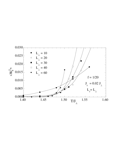
Figure 5: Plot of z axis winding $\langle W_{z}^{2}\rangle$ vs. $T/J_{\perp}$ for $L_{\perp}=10$, $20$, $30$, $40$, and $60$, with vortex density $f=1/20$, anisotropy $J_{z}=0.02J_{\perp}$, and aspect ratio $L_{z}=L_{\perp}$. $\langle W_{z}^{2}\rangle$ is computed using method (iii), i.e. first find all loops that percolate in the negative $\hat{z}$ direction. Solid lines are guides to the eye only.

Figure 6: Plot of z axis winding $\langle W_{z}^{2}\rangle$ vs. $T/J_{\perp}$ for $L_{\perp}=20$, $30$, $40$, $60$, $100$ and $120$, with vortex density $f=1/20$, anisotropy $J_{z}=0.02J_{\perp}$, and aspect ratio $L_{z}=L_{\perp}/5$. $\langle W_{z}^{2}\rangle$ is computed using method (iii), i.e. first find all loops that percolate in the negative $\hat{z}$ direction. Solid lines are guides to the eye only.

IV Percolating Loops

IV.1 Summary of Sudbø’s Method

As discussed in the preceding Section III.A, a transition at $T_{\Phi}$ would mark the appearance of infinite transverse loops, as $T$ is increased. The idea to explicitly look for transverse paths that percolate across the system was first put forth by Jagla and Balseiro.R16 Later, Sudbø and co-workersR6 ; R7 ; R8 refined this idea. They defined a quantity which they denoted $O_{L}$, which is the probability that a vortex path exists which travels completely across the system in a direction transverse to the applied magnetic field, without ever traveling completely across the system in the direction parallel to the field. If such a path exists in a given configuration, that configuration counts as unity in the average for $O_{L}$; if not, that configuration counts as zero.

Since having $W^{2}>0$ in a given configuration necessarily implies that there is a percolating transverse loop in that configuration, there is a close connection between the quantities $\langle W^{2}\rangle$ and $O_{L}$. They differ in that (i) for a configuration with $W^{2}>1$, and hence with more than one percolating transverse loop, the contribution to $O_{L}$ remains unity, rather than increasing with the number of percolating transverse loops; and (ii) in a configuration with two percolating but oppositely oriented transverse loops, the contribution to $O_{L}$ will be unity, but these loops cancel each other in their contribution to $W^{2}$, which might therefore be zero.

Since $O_{L}$ is a pure number one might expect it to be a scale invariant quantity, and hence, similar to $\langle W^{2}\rangle$, plots of $O_{L}$ vs. $T$ for different system sizes $L_{\perp}$ should have a common intersection point at $T_{\Phi}$.

Sudbø and co-workers’ method of searching for such percolating transverse paths is similar to our method (ii) except for one crucial difference.R17 They do not require that the transverse path closes upon itself; they only require that the path start at one end of the system, say at $x=0$, and continue until reaching the opposite end, $x=L_{\perp}$, while keeping the distance traveled along $\hat{z}$ less than $L_{z}$, that is the displacement traveled along the path $\alpha$ satisfies $R_{x\alpha}=L_{\perp}$ and $R_{z\alpha}<L_{z}$. Since, by the periodic boundary conditions, all paths must eventually close upon themselves, there are two possibilities for the transverse percolating paths that Sudbø and co-workers find. We illustrate these in Fig. 7: (1) the path $\alpha$ eventually closes upon itself without ever traveling the length $L_{z}$, in which case $R_{z\alpha}=0$; or (2) the path $\alpha$, when followed until it closes upon itself, does wind up traveling the length $L_{z}$, with a displacement $R_{z\alpha}=L_{z}$; in this case, our method (ii) would consider this path as part of the field induced vortex lines $n_{s\mu}^{\mathrm{lines}}$, contributing to the winding ${\bf W}$, rather than as a transverse loop that contributes to $n_{s\mu}^{\mathrm{loops}}$. We will call Sudbø’s path tracing method (ii^′) to distinguish it from our method (ii). The probability for a percolating path using method (ii^′) we will denote by $O_{L}^{\prime}$; using method (ii) we will denote it by $O_{L}$. Paths of type (2) will contribute to $O_{L}^{\prime}$, but not to $O_{L}$. We will see that there are very dramatic differences between these two methods, and that only $O_{L}$ gives self-consistent results.

Figure 7: Examples of percolating transverse vortex paths. Path (1) closes upon itself without ever winding about the system in the $\hat{z}$ direction. Path (2) only closes upon itself after winding once in the $\hat{z}$ direction. Both paths contribute to the calculation of $O_{L}^{\prime}$ by method (ii^′). Only path (1) contributes to the calculation of $O_{L}$ by method (ii). The thin dashed lines represent the periodic boundaries of the system.

IV.2 Numerical Results

First, we note that if we use method (i) (random connections) to search for percolating transverse paths, the result is essentially the same as found for $\langle W^{2}\rangle$ in section III.B. As $L_{\perp}$ increases, the probability to find a percolating transverse loop steadily decreases for the entire temperature range, becoming immeasurably small for our biggest system size. Hence we will focus here on methods (ii) and (ii^′).

We now consider the computation of $O_{L}^{\prime}$ using method (ii^′), the one used by Sudbø and co-workers, which never checks to see how the percolating transverse path closes upon itself. We first use parameters $J_{z}=0.02J_{\perp}$ and $L_{z}=L_{\perp}$, the same as in section III.B, but a more dilute density of vortex lines $f=1/90$. For these parameters, the vortex lattice melting temperature is $T_{m}\simeq 0.49J_{\perp}$, and the zero field critical temperature, as before, is $T_{c0}\simeq 1.14J_{\perp}$. These parameters are very close to the parameters of one of the cases studied by Sudbø and co-workers in Refs. R7, and R8, (they used $f=1/90$, $J_{z}=(1/49)J_{\perp}$ and $L_{z}\sim L_{\perp}$). Our results for $O_{L}^{\prime}$ vs $T/J_{\perp}$, for three system sizes, $L_{\perp}=30$, $60$ and $90$, are shown as the solid symbols on the left hand side of Fig. 8. These results agree quite closely with those of Sudbø and co-workers (see Fig. 8 of Ref. R7, ), and seem to show what might be a common intersection of the three curves near $T\simeq 0.7J_{\perp}$. However, we now consider the same parameters and sizes $L_{\perp}$, only using a different system aspect ratio, $L_{z}=L_{\perp}/6$. The results are shown as the open symbols on the right hand side of Fig. 8. We see that there no longer appears to be a common intersection point, but more importantly, the curves have all shifted dramatically to higher temperatures. Thus, any value of $T_{\Phi}$ that one might try to extract from $O_{L}^{\prime}$ depends sensitively on the system aspect ratio. We have also considered other values of the aspect ratio $L_{z}/L_{\perp}$, not shown here. The clear trend is that the sharp rise in $O_{L}^{\prime}$ shifts to increasing temperatures as $L_{z}/L_{\perp}$ decreases. But if $T_{\Phi}$ represents a true phase transition, it must be independent of aspect ratio. We therefore conclude that $O_{L}^{\prime}$ and method (ii^′) do not give any self-consistent evidence of the proposed vortex loop blowout transition.

Figure 8: Plot of percolation probability $O_{L}^{\prime}$ vs. $T/J_{\perp}$ for $L_{\perp}=30$, $60$, and $90$, with vortex density $f=1/90$, and anisotropy $J_{z}=0.02J_{\perp}$. Solid symbols on the left are for aspect ratio $L_{z}=L_{\perp}$; open symbols on the right are for aspect ratio $L_{z}=L_{\perp}/6$. $O_{L}^{\prime}$ is computed using method (ii^′), following Sudbø and co-workers. Solid lines are guides to the eye only.

The problems with $O_{L}^{\prime}$ are even clearer if we consider the parameters $f=1/20$ and $J_{z}=0.02J_{\perp}$, the same ones used for our computation of $\langle W^{2}\rangle$ in section III.B. In Fig. 9 we show our results for $L_{\perp}=10$, $20$, and $40$, for the two aspect ratios $L_{z}=L_{\perp}$ and $L_{z}=L_{\perp}/2$. In both cases, there is no common intersection point of the three curves for the three sizes, and the curves for the smaller aspect ratio are shifted to higher temperatures. Note also that, for both aspect ratios, the temperatures at which $O_{L}^{\prime}$ rises to unity lie quite significantly below the value of $T_{\Phi}\simeq 1.4J_{\perp}$ found from our analysis of $\langle W^{2}\rangle$.

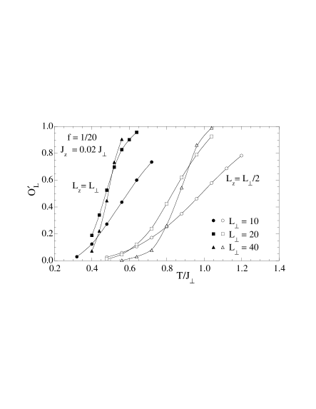
Figure 9: Plot of percolation probability $O_{L}^{\prime}$ vs. $T/J_{\perp}$ for $L_{\perp}=10$, $20$, and $40$, with vortex density $f=1/20$, and anisotropy $J_{z}=0.02J_{\perp}$. Solid symbols on the left are for aspect ratio $L_{z}=L_{\perp}$; open symbols on the right are for aspect ratio $L_{z}=L_{\perp}/2$. $O_{L}^{\prime}$ is computed using method (ii^′), following Sudbø and co-workers. Solid lines are guides to the eye only.

We next consider the the computation of $O_{L}$ using method (ii) (percolating transverse path must close upon itself keeping $R_{z\alpha}=0$). In Fig. 10 we show results using the same parameters as were used to compute $O_{L}^{\prime}$in Fig. 8, i.e. $f=1/90$, $J_{z}=0.02J_{\perp}$, and $L_{\perp}=30$, $60$ and $90$, for the same two aspect ratios $L_{z}=L_{\perp}$ and $L_{z}=L_{\perp}/6$. We see now that for both aspect ratios, curves for the three different sizes appear to approach a common intersection point, $T_{\Phi}\simeq 1.17J_{\perp}>T_{c0}\simeq 1.14J_{\perp}$, and that this intersection point is independent of aspect ratio (note: for $L_{z}=L_{\perp}/6$, the thinness of the system $L_{z}=5$, for $L_{\perp}=30$, presumably makes it too small to be in the scaling region, hence it intersects the other two curves at somewhat lower temperatures).

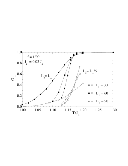
Figure 10: Plot of percolation probability $O_{L}$ vs. $T/J_{\perp}$ for $L_{\perp}=30$, $60$, and $90$, with vortex density $f=1/90$, and anisotropy $J_{z}=0.02J_{\perp}$. Solid symbols are for aspect ratio $L_{z}=L_{\perp}$; open symbols are for aspect ratio $L_{z}=L_{\perp}/6$. $O_{L}$ is computed using method (ii), where all loops close upon themselves. All curves approach a common intersection point, $T_{\Phi}\simeq 1.17J_{\perp}$, independent of the aspect ratio. Solid lines are guides to the eye only.

In Fig. 11 we show similar results using the same parameters as were used in our computation of $\langle W^{2}\rangle$ in section III.B, i.e. $f=1/20$, $J_{z}=0.02J_{\perp}$ and $L_{z}=L_{\perp}$. We see that the curves of $O_{L}$ vs. $T/J_{\perp}$ for the different system sizes, $L_{\perp}=10$, $20$, $30$ and $40$, all intersect at a common point, $T_{\Phi}\simeq 1.4J_{\perp}$. This is exactly the same value as found in our analysis of $\langle W^{2}\rangle$ (see Fig. 2).

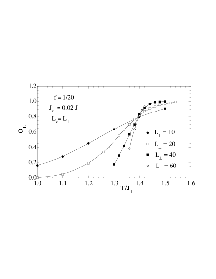
Figure 11: Plot of percolation probability $O_{L}$ vs. $T/J_{\perp}$ for $L_{\perp}=10$, $20$, $40$, and $60$, with vortex density $f=1/20$, anisotropy $J_{z}=0.02J_{\perp}$, and aspect ratio $L_{z}=L_{\perp}$. $O_{L}$ is computed using method (ii), where all loops close upon themselves. All curves approach a common intersection point, $T_{\Phi}\simeq 1.4J_{\perp}$, in agreement with the analysis of $\langle W^{2}\rangle$ in Fig. 2. Solid lines are guides to the eye only.

We therefore conclude that $O_{L}$ gives a self-consistent determination of $T_{\Phi}$, and that this value is considerably larger than estimates one would get from consideration of $O_{L}^{\prime}$. In fact, estimates of a $T_{\Phi}$ from $O_{L}^{\prime}$ all lie below the zero field critical temperature $T_{c0}$ and decrease as $f$ increases, while the values determined from $O_{L}$ all lie above $T_{c0}$, and increase as $f$ increases.

If $O_{L}$ is indeed a scale invariant quantity, we can postulate that it should obey a scaling relation similar to $\langle W^{2}\rangle$, i.e.,

$$O_{L}(T,L_{\perp})=\tilde{f}(tL^{1/\nu})$$ (15)

Based on our analysis of $\langle W^{2}\rangle$ in section III.B, we may expect $\nu\simeq 1$. In Fig. 12 we therefore show a scaling collapse of the data for $f=1/90$ from Fig. 10, plotting $O_{L}$ vs. $[(T-T_{\Phi})/J_{\perp}]L_{\perp}$, where $T_{\Phi}$ is determined by a best fit of the data to the scaling form. We find a reasonably good collapse for all sizes, for both aspect ratios, using a single value of $T_{\Phi}\simeq 1.168J_{\perp}$.

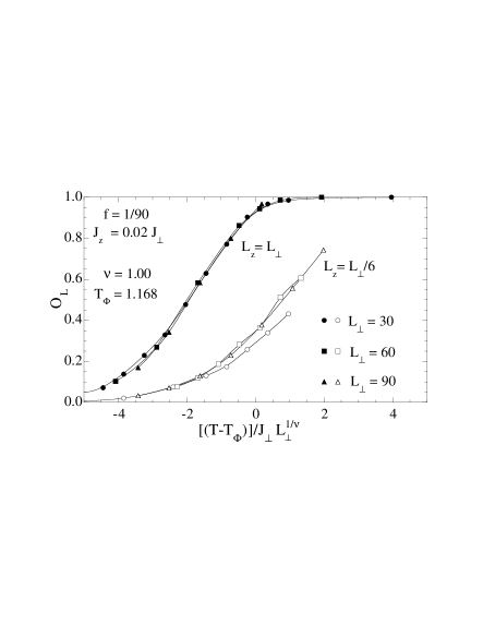
Figure 12: Scaling collapse $O_{L}$ vs. $[(T-T_{\Phi})/J_{\perp}]L_{\perp}^{1/\nu}$ of data from Fig. 10, for $f=1/90$. A reasonably good collapse is found for all sizes $L_{\perp}$, for both aspect ratios $L_{z}/L_{\perp}$, using a single value of $T_{\Phi}\simeq 1.168J_{\perp}$ and $\nu=1$. Solid lines are guides to the eye only.

In Fig. 13 we show a similar scaling collapse of the data for $f=1/20$ from Fig. 11. Fitting the data for $O_{L}$ to a 4th order polynomial expansion of the scaling function, we find an excellent collapse, for all system sizes, using the parameters $T_{\Phi}\simeq 1.399J_{\perp}$ and $\nu=1.006$. These results agree very well with the values obtained from the scaling analysis of $\langle W^{2}\rangle$, given in section III.B. The quality of the collapse is very much better here than it was for $\langle W^{2}\rangle$ in Fig. 4.

Figure 13: Scaling collapse $O_{L}$ vs. $[(T-T_{\Phi})/J_{\perp}]L_{\perp}^{1/\nu}$ of data from Fig. 11, for $f=1/20$. An excellent collapse is found for all sizes $L_{\perp}$, using a value of $T_{\Phi}\simeq 1.399J_{\perp}$ and $\nu=1.006$. These values agree well with those obtained from the scaling collapse of $\langle W^{2}\rangle$. The solid line is the fitted polynomial curve.

Finally, in analogy with the winding $\langle W_{z}^{2}\rangle$, we have also considered the probability $O_{Lz}$ to find a vortex path percolating through the system in the negative $\hat{z}$ direction, opposite to the applied magnetic field. We expect $O_{Lz}$ to obey a scaling relation similar to that of Eq. (15). To compute $O_{Lz}$ we have used tracing method (iii) in which we explicitly search through all possible connections to find any such paths. We show our results for $O_{Lz}$ vs. $T/J_{\perp}$ for vortex density $f=1/20$ and anisotropy $J_{z}=0.02J_{\perp}$ in Figs. 14 and 15, for system aspect ratios $L_{z}=L_{\perp}$ and $L_{z}=L_{\perp}/5$ respectively. As with $\langle W_{z}^{2}\rangle$ shown in Figs. 5 and 6, the intersection points of the curves for different sizes appear to decrease in temperature as $L_{\perp}$ increases. Again, we cannot say if this is a failure of our scaling hypothesis, or a failure to reach sufficiently large $L_{z}$. Also, analogous to our findings for the windings $\langle W^{2}\rangle$ and $\langle W_{z}^{2}\rangle$, $O_{Lz}$ appears to be vanishing at a temperature above the $T_{\Phi}=1.4J_{\perp}$ where the curves of $O_{L}$ intersect.

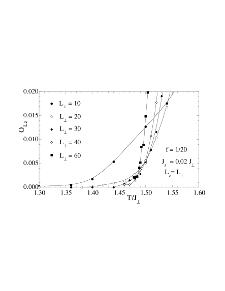
Figure 14: Plot of percolation probability $O_{Lz}$ vs. $T/J_{\perp}$ for $L_{\perp}=10$, $20$, $30$, $40$, and $60$, with vortex density $f=1/20$, anisotropy $J_{z}=0.02J_{\perp}$, and aspect ratio $L_{z}=L_{\perp}$. $O_{Lz}$ is computed using tracing method (iii). Solid lines are guides to the eye only.

Figure 15: Plot of percolation probability $O_{Lz}$ vs. $T/J_{\perp}$ for $L_{\perp}=20$, $30$, $40$, $60$, $80$, and $100$, with vortex density $f=1/20$, anisotropy $J_{z}=0.02J_{\perp}$, and aspect ratio $L_{z}=L_{\perp}/5$. $O_{Lz}$ is computed using tracing method (iii). Solid lines are guides to the eye only.

V Specific Heat

If $T_{\Phi}$, as determined by $\langle W^{2}\rangle$ or $O_{L}$, does indeed represent a true thermodynamic transition, we would expect to see some signature of this transition in more conventional thermodynamic quantities. In the recent experiments of Ref.R9, , a step like anomaly in the specific heat $C$ was observed in the vortex line liquid region, reminiscent of an inverted mean field transition. In their numerical simulations,R7 ; R8 Nguyen and Sudbø claimed to see an anomalous glitch in the specific heat at the temperature they identified as $T_{\Phi}$ from their calculation of $O_{L}^{\prime}$. However, this glitch corresponded to only a single data point very slightly displaced above an otherwise smooth background; and in the previous section we have demonstrated that $O_{L}^{\prime}$ significantly underestimates $T_{\Phi}$, hence there is no reason to expect any anomaly in $C$ at that temperature.

In this section we report on high precision measurements of the specific heat $C$, for the same parameters we have studied in the earlier sections. If the $T_{\Phi}$, as found using the vortex path tracing method (ii), is indeed a true thermodynamic phase transition with critical exponent $\nu\simeq 1$ (as our scaling analyses found), then hyperscaling would suggest a specific heat exponent of $\alpha=2-d\nu\simeq-1$. We thus do not expect to see a diverging $C$, however some feature should be present.

In Fig. 16 we plot $C$ vs. $T/J_{\perp}$, in the near vicinity of $T_{\Phi}\simeq 1.4J_{\perp}$, for the same parameters $f=1/20$, $J_{z}=0.02J_{\perp}$, and $L_{z}=L_{\perp}$ as used in Figs. 2, 11 and 13. We show results for $L_{\perp}=10$, $20$, $30$ and $40$, using from $3-10\times 10^{7}$ Monte Carlo passes through the lattice, depending on the system size. We find no noticeable finite size dependence, and no hint of any feature at all, near the previously determined $T_{\Phi}\simeq 1.4J_{\perp}$.

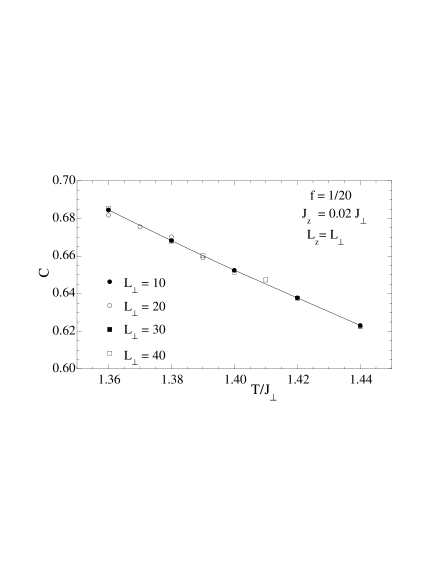
Figure 16: Specific heat $C$ vs. $T/J_{\perp}$ for vortex density $f=1/20$, anisotropy $J_{z}=0.02J_{\perp}$, and aspect ratio $L_{z}=L_{\perp}$, for system sizes $L_{\perp}=10$, $20$, $30$ and $40$. No hint of any anomaly is found near the previously determined $T_{\Phi}\simeq 1.4J_{\perp}$. The solid line is a guide to the eye only.

In Fig. 17 we plot $C$ vs. $T/J_{\perp}$, over a broad temperature range, for the same parameters $f=1/90$ and $J_{z}=0.02J_{\perp}$ as used in Figs. 10 and 12, but for a single large system size $L_{\perp}=30$ and $L_{z}=90$. Again we see no hint of any anomaly near the previously determined $T_{\Phi}\simeq 1.168J_{\perp}$.

Figure 17: Specific heat $C$ vs. $T/J_{\perp}$ for vortex density $f=1/90$, anisotropy $J_{z}=0.02J_{\perp}$, and aspect ratio $L_{z}=3L_{\perp}$, for system size $L_{\perp}=30$. No hint of any anomaly is found near the previously determined $T_{\Phi}\simeq 1.168J_{\perp}$. The solid line is a guide to the eye only.

VI Conclusions

We have carried out detailed Monte Carlo investigations of the 3D uniformly frustrated XY model in order to search for a proposed “vortex loop blowout” transition within the vortex line liquid phase of a pure extreme type-II superconductor. Such a transition had been predicted from general theoretical arguments by Tešanović.R5 Evidence for such a transition was claimed in numerical simulations by Sudbø and co-workers,R6 ; R7 ; R8 and in specific heat measurements on high purity YBCO single crystals.R9 We have made explicit measurements of the vortex line windings $\langle W^{2}\rangle$ and $\langle W_{z}^{2}\rangle$, which are the key quantities in Tešanović’s theory. We have re-examined Sudbø’s calculation of the percolation probability $O_{L}$.

Our results raise several questions concerning Tešanović’s theory. We have found that the values of $\langle W^{2}\rangle$ and $\langle W_{z}^{2}\rangle$ depend sensitively on the precise scheme one uses to trace out vortex line paths. For the natural choice of random connectivity at vortex line intersections, both $\langle W^{2}\rangle$ and $\langle W_{z}^{2}\rangle$ appear to vanish at all temperatures as $L\to\infty$. Only when we specifically search first for percolating paths, when computing the windings, do we find that the windings converge to non zero values above a certain temperature. In this case, we find that the transverse winding $\langle W^{2}\rangle$ obeys the finite size scaling form expected from Tešanović’s theory, however the critical exponent we find is $\nu\simeq 1$, rather than the predicted $\nu_{XY}\sim 2/3$ of the inverted 3D XY transition. For the longitudinal winding $\langle W_{z}^{2}\rangle$ we have been unable to find the expected scaling form. Whether this is because $\langle W_{z}^{2}\rangle$ does not scale, or because our systems are all too small to be in the scaling limit, we cannot be certain. It does appear that, upon cooling, $\langle W_{z}^{2}\rangle$ vanishes at a temperature above that where $\langle W^{2}\rangle$ vanishes. This would be contrary to Tešanović’s theory. However, since we have not succeeded to find scaling for $\langle W_{z}^{2}\rangle$, we cannot be certain of knowing exactly where it vanishes as $L\to\infty$.

Independent of Tešanović’s theory, it is natural to think that, as temperature and hence vorticity increases, the vortex lines may form percolating paths (note however that the directedness of the vortex line segments, and the condition of divergenceless paths, means that this is no ordinary percolation problem!). We have therefore, following Sudbø and co-workers, searched explicitly for such percolating paths in the direction transverse to the applied magnetic field, as well as in the direction parallel but opposite to the applied magnetic field. Defining transverse percolation as the existence of a vortex line path that extends entirely across the system in the direction transverse to the applied magnetic field without simultaneously extending entirely across the system in the parallel direction, we have shown that Sudbø’s procedure, which ignores the transverse periodic boundary conditions and does not require the percolating path to close upon itself, leads to inconsistent predictions for the transition temperature as one varies the system aspect ratio. Only by requiring that the transverse percolating path close upon itself, without ever winding in the parallel direction, do we find a consistent transition temperature independent of aspect ratio. The percolation transition found this way agrees both in critical temperature $T_{\Phi}$ and exponent $\nu$ with the results from our analysis of the transverse winding $\langle W^{2}\rangle$. We have also computed the probability to find a percolating path in the direction parallel but opposite to the applied magnetic field. Here, analogous to our results for $\langle W_{z}^{2}\rangle$, this negative $\hat{z}$ percolation appears to occur at a temperature higher than that of the transverse percolation, however we have not succeeded to find a clear scaling of this parallel percolation probability.

Note that the transverse percolation transition temperature $T_{\Phi}(f)$ that we find increases above the zero field transition temperature $T_{c0}$ as the magnetic flux density $f$ increases. This is in striking contrast to the conclusion of Sudbø and co-workers who proposed $T_{\Phi}(f)$ to decrease below $T_{c0}$ as $f$ increases.

While our results do seem consistent with a well defined transverse percolation transition, one can ask if this is a purely geometrical feature of the vortex line paths, or whether it also corresponds to a true thermodynamic phase transition, i.e. something one could detect in a suitable thermodynamic derivative of the free energy. To investigate this question we have carried out high precision Monte Carlo measurements of the specific heat $C$. Our results for $C$ show no feature whatsoever near the percolation transition $T_{\Phi}$, nor do we find any finite size effect. In particular we see no evidence for a step like feature as was observed experimentally in YBCO.

To conclude, we have found evidence for a well defined transverse percolation temperature within the vortex line liquid phase of a model type-II superconductor. The connection between this transition and Tešanović’s theory of a vortex loop “blowout” transition remains unclear. It also remains unclear whether or not this percolation transition has any observable thermodynamic manifestation.

References

- (1) E. Zeldov et al., Nature 375, 373 (1995); A. Schilling et al., Nature 382, 791 (1996).
- (2) M. V. Feigel’man, V. B. Geshkenbein, L. B. Ioffe and A. I. Larkin, Phys. Rev. B 48, 16641 (1993).
- (3) Y.-H. Li and S. Teitel, Phys. Rev. B 47, 359 (1993).
- (4) Y.-H. Li and S. Teitel, Phys. Rev. B 49, 4136 (1994).
- (5) T. Chen and S. Teitel, Phys. Rev. B 55, 11766 (1997).
- (6) X. Hu, S. Miyashita and M. Tachiki, Phys. Rev. Lett. 79, 3498 (1997) and Phys. Rev. B 58 3438 (1998); A. K. Nguyen and A. Sudbø, Phys. Rev. B 58, 2802 (1998); P. Olsson and S. Teitel, Phys. Rev. Lett. 82, 2183 (1999).
- (7) Z. Tešanović, Phys. Rev. B 59, 6449 (1999) and Phys. Rev. B 51, 16204 (1995).
- (8) S. K. Chin, A. K. Nguyen and A. Sudbø, Phys. Rev. B 59, 14017 (1999).
- (9) A. K. Nguyen and A. Sudbø, Europhys. Lett. 46, 780 (1999).
- (10) A. K. Nguyen and A. Sudbø, Phys. Rev B 60, 15307 (1999).
- (11) F. Bouquet et al., Nature 411, 448 (2001).
- (12) Y.-H. Li and S. Teitel, Phys. Rev. Lett. 66, 3301 (1991).
- (13) P. Olsson, Europhys. Lett. 58, 705 (2002).
- (14) For large systems, it is crucial to have an efficient algorithm to search for such paths. We use the following. First, all intersection points are located. Picking one such point at random, we trace out a path starting from this intersection point until it arrives at another intersection point. If the height traveled from the starting to the new intersection point is , we stop this search and start again at a different intersection point; if not, we continue tracing the path until then next intersection point is encountered and then repeat the height test. Since most paths connect to field lines which travel in the direction, most such tracings are quickly aborted. However, since each possible transverse loop with contains an intersection point that is at the largest height of all intersection points on that loop, we are guarenteed to ultimately find this path with this search algorithm.
- (15) C. Dasgupta and B. I. Halperin, Phys. Rev. Lett. 47, 1556 (1981).
- (16) E. Fradkin, B. A. Huberman, and S. H. Shenker, Phys. Rev. B 18, 4789 (1978); G. Carneiro, Phys. Rev. B 45, 2391 (1992).
- (17) T. Chen and S. Teitel, Phys. Rev. B 55, 15197 (1997).
- (18) M. Kiometzis, H. Kleinert, and A. M. J. Schakel, Fortschr. Phys. 43, 697 (1995).
- (19) P. Olsson and S. Teitel, Phys. Rev. Lett. 80, 1964 (1998).
- (20) D. R. Nelson, Phys. Rev. Lett. 60, 1973 (1988); J. Stat. Phys. 57, 511 (1989); D. R. Nelson and H. S. Seung, Phys. Rev. B 39, 9153 (1989).
- (21) E. A. Jagla and C. A. Balseiro, Phys. Rev. B 53, R538 (1996); ibid. 53, 15305. In these works, the authors considered all transverse percolating loops, including those with net winding in the parallel direction, . One can show that the onset of such loops, which in general involve the participation of the field induced lines and so do have , coincides with the vanishing of the longitudinal helicity modulus and so occurs at the melting , rather than the proposed . Only by restricting to loops with does one probe .
- (22) A. Sudbø, private communication.