Optimization and Physics: On the satisfiability of random Boolean formulae

Abstract

LECTURE GIVEN AT TH2002: Given a set of Boolean variables, and some constraints between them, is it possible to find a configuration of the variables which satisfies all constraints? This problem, which is at the heart of combinatorial optimization and computational complexity theory, is used as a guide to show the convergence between these fields and the statistical physics of disordered systems. New results on satisfiability, both on the theoretical and practical side, can be obtained thanks to the use of physics concepts and methods.

Combinatorial optimization aims at finding, in a finite set of possible configurations, the one which minimizes a certain cost function. The famous example of the traveling salesman problem (TSP) can serve as an illustration: A salesman must make a tour through $N$ cities, visiting each city only once, and coming back at its starting point. The cost function is a symmetric matrix $c_{ij}$, where $c_{ij}$ is the cost for the travel between cities $i$ and $j$. A permutation $\pi$ of the $N$ cities gives a tour $\pi(1)\to\pi(2)\to\pi(3)\to...$. Taking into account the equivalence between various starting points and the direction of the tour, one sees that the number of distinct tour is $(N-1)!/2$. For each tour $\pi$, the total cost is $C=c_{\pi(N)\pi(1)}+\sum_{r=1}^{N-1}c_{\pi(r)\pi(r+1)}$, which can be computed in $N$ operations. The problem is to find the tour $\pi$ with lowest cost.

As can be seen on this example, the basic ingredients of the optimization problems which will interest us are the following:

• An integer $N$ giving the size of the problem (in the TSP, it is the number of cities).

• A set of configurations, which typically scales like $\exp(N^{\alpha})$.

• A cost function, which one can compute in polynomial time $O(N^{\gamma})$.

Let me mention a few examples, beside the TSP papad .

In the assignment problem, one is given a set of $N$ persons $i=1,...,N$, a set of $N$ tasks $a=1,...,N$, a $N\times N$ cost matrix $c$ where $c_{ia}$ is the cost for having task $a$ performed by person $i$. An assignment is a permutation $\pi\in S_{N}$ assigning task $a=\pi(i)$ to person $i$, and the problem is to find the lowest cost assignment, i.e. the permutation which minimizes $C=\sum_{i=1}^{N}c_{i\pi(i)}$.

In the spin glass problemMPV , one is given a set of $N$ spins, which could be for instance Ising variables $\sigma_{i}\in\{\pm 1\}$, the total energy of the configuration is a sum of exchange interaction energies between all pairs of spins, $E(\{\sigma\})=-\sum_{1\leq i<j\leq N}J_{ij}\sigma_{i}\sigma_{j}$, and one seeks the ground state of the problem, i.e. the configuration (among the $2^{N}$ possible ones) which minimizes the energy.

In physical terms, optimization problems consist in finding ground states. This task can be non trivial if a system is frustrated, which means that one cannot get the ground state simply by minimizing the energy locally. This is typically what happens in a spin glass. In some sense, statistical physics addresses a more general question. Assuming that the system is at thermal equilibrium at temperature $T$, every configuration ${\cal C}$ is assigned a Boltzmann probability, $P({\cal C})=\frac{1}{Z}e^{-{\beta}{E({\cal C})}}$. Beside finding the ground state, one can ask also interesting questions about which are the typical configurations at a given temperature, like counting them (which leads to the introduction of entropy), or trying to know if they are located in one single region of phase space, or if they build up well separated clusters, as often happens in situation where ergodicity is broken. The generalization introduced by using a finite temperature, beside leading to interesting questions, can also be useful for optimization, both from the algorithmic point of view (for instance this is the essence of the simulated annealing algorithmKGV , which is a general purpose heuristic algorithm that can be used in many optimization problems), but also from an analytic point of view MPV . Conversely, smart optimization algorithms turn out to be very useful in the study of frustrated physical systems like spin glasses or random field models, and the cross-fertilization between these two fields (and also with the related domain of error correcting codes for information transmission codes ) has been very fruitful in the recent years TCS_issue .

Before proceeding with one such example, let us briefly mention a few important results in optimization which will provide the necessary background and motivation. One of the great achievements of computer science is the theory of computational complexity. It is impossible to present it in any details here and I will just sketch a few main ideas, the interested reader can study it for instance in papad2 .

Within the general framework explained above, we can define three types of optimization problems: the optimization problem in which one wants to find the optimal configuration, the evaluation problem in which one wants to compute the optimal cost (i.e. the ground state energy), the decision problem in which one wants to know, given a threshold cost $C_{0}$, if there exists a configuration of cost less than $C_{0}$.

One classification of decision problems is based on the scaling with $N$ of the computer time required to solve them in the worst case. There are two main complexity classes:

• Class P   = polynomial problems: they can be solved in a time $t<N^{\alpha}$. The assignment is an example of a polynomial problem, as is the spin glass problem in 2 dimensions.

• Class NP = non-deterministic polynomial: Given a ’yes’ solution to a NP problem, it can be checked in polynomial time. Roughly speaking this means that the energy is computable in polynomial time, so this class contains a wide variety of problems, including most of the ones of interest in physics. All problems mentioned above are in NP.

One nice aspect of focusing on polynomiality is that it allows to forget about the details of the definition of $N$, the implementation, language, machine, etc…: any ’reasonable’ such change (for instance one could have used the number of possible links in the assignment) will change the exponent of $N$ appearing in the computer time of a problem in P, but not transform it into an exponential behavior. A problem $A$ is said to be at least as hard as a problem $B$ if there exists a polynomial algorithm which transforms any instance of $B$ into an instance of $A$.

This allows to define the very important class:

• NP-complete A problem is NP complete if it is at least as hard as any problem in NP.

So the NP-complete are the hardest problems in NP. If one such problem can be solved in polynomial time, then all the problems in NP are solved in polynomial time. Clearly P is contained in NP, but it is not yet known whether P = NP , and this is considered as a major challenge.

A great result was obtained in this field by Cook in 1971 Cook : The satisfiability problem, which we shall describe below, is NP-complete. Since then hundreds of problems have been shown to belong to this class, among which the decision TSP or the spin glass in dimension larger or equal to 3.

The fact that 3-d spin glass is NP-complete while 2-d spin glass is P might induce one to infer that NP-completeness is equivalent with the existence of a glass transition. This reasoning is too naive and wrong; the reason is that the complexity classification relies on a worth-case analysis, while physicists study the behavior of a typical sample. The development of a typical case complexity theory has become a major goal average , also motivated by the experimental observations that many instances of NP-complete problems are easy to solveTCS_issue .

One way of addressing this issue of a typical case complexity is to define a probability measure on the instances (= the ’samples’) of the optimization problem which one is considering. Typical examples are:

• TSP with independent random points uniformly distributed in the unit square

• assignment with independent affinities uniformly distributed on $[0,1]$

• CuMn spin glass at one percent Mn

Once this measure has been defined, one is interested in the properties of the generic sample in the $N\to\infty$ limit. In most cases, global properties (e.g. extensive thermodynamic quantities, among which the ground state energy), turn out to be self averaging. This means for instance that the distribution of the ground state energy density becomes more and more peaked around an asymptotic value in the large $N$ limit: almost all samples have the same ground state energy density. In this situation, a statistical physics analysis is appropriate. Early examples of the use of statistical physics in such a context are the derivation of bounds for the optimal length of a TSPMVan , the exact prediction of the ground state energy in the random assignment problem defined above, where the result $E_{0}=\frac{\pi^{2}}{6}$, derived in 1985 through a replica analysisMP_match , was recently confirmed rigorously by Aldous Aldous , or the link between spin glasses and graph partitioning FuAnd .

As statistical physics can be quite powerful at understanding the generic structure of an optimization problem, one may also hope that it can help finding better optimization algorithms. A successful example which was developed recently is the satisfiability problem, to which we now turn.

As we have seen, satisfiability is a core problem in optimization and complexity theory. It is defined as follows Hayes : A configuration is a set of $N$ Boolean variables $x_{i}\in\{0,1\}\quad i=1,\ldots,N$. One is given $M$ constraints which are clauses, meaning that they are in the form of an OR function of some variables or their negations. For instance: $x_{1}\vee x_{27}\vee\bar{x}_{3}$, $\bar{x}_{11}\vee x_{2}$, are clauses (notation: $\bar{x}_{3}$ is the negation of $x_{3}$). So the clause $x_{1}\vee x_{27}\vee\bar{x}_{3}$ is satisfied if either $x_{1}=1$, or $x_{27}=1$, or $x_{3}=0$ (these events do not exclude each other). The satisfiability problem is a decision problem. It asks whether there exists a choice of the Boolean variables such that all constraints are satisfied (we will call it a SAT configuration). This is a very generic problem, because one can see it as finding a configuration of the $N$ Boolean variables which satisfies the logical proposition built from the AND of all the clauses (in our example $(x_{1}\vee x_{27}\vee\bar{x}_{3})\wedge(\bar{x}_{11}\vee x_{2})\wedge\ldots$), and any logical proposition can be written in such a ’conjunctive normal form’ .

Satisfiability is known to be NP complete if it contains clauses of length $\geq 3$, but common sense and experience show that the problem can often be easy; for instance if the number of constraints per variable $\alpha=\frac{M}{N}$ is small, the problem is often SAT, if it is large, the problem is often UNSAT.

This behavior can be characterized quantitatively by looking at the typical complexity of the random 3-SAT problem, defined as follows. Each clause involves exactly three variables, chosen randomly in $\{x_{1},..,x_{N}\}$; a variable appearing in the clause is negated randomly with probability $1/2$. This defines the probability measure on instances for the random 3-SAT problem. The control parameter is the ratio Constraints/Variables $\alpha=\frac{M}{N}$ .

The properties of random 3-SAT have been first investigated numerically KirkSel ; Crawford , and exhibit a very interesting threshold phenomenon at $\alpha_{c}\sim 4.26$: a randomly chosen sample is generically SAT for $\alpha<\alpha_{c}$ (meaning that it is SAT with probability $1$ when $N\to\infty$), generically UNSAT for $\alpha>\alpha_{c}$. The time used by the best available algorithms (which have an exponential complexity) to study the problem also displays an interesting behavior: For $\alpha$ well below $\alpha_{c}$, it is easy to find a SAT configuration; for $\alpha$ well above $\alpha_{c}$, it is relatively easy to find a contradiction in the constraints, showing that the problem is UNSAT. The really difficult region is the intermediate one where $\alpha\sim\alpha_{c}$, where the computer time requested to solve the problem is much larger and increases very fast with system size. A lot of important work has been done on this problem, to establish the existence of a threshold phenomenon, give upper and lower bounds on $\alpha_{c}$, show the existence of finite size effects around $\alpha\sim\alpha_{c}$ with scaling exponents. We refer the reader to the literature KirkSel ; Crawford ; MZKST ; bounds_1 ; bounds_2 ; bounds_3 ; bounds_4 , and just here extract a few crucial aspects for our discussion. The threshold phenomenon is a phase transition, and the neighborhood of the transition is the region where the algorithmic problem becomes really hard.

This relationship between phase transition and complexity makes a statistical physics analysis of this problem particularly interesting. Monasson and Zecchina have been the first ones to recognize this importance and to use statistical physics methods for an analytic study of the random 3-SAT problem MoZe_prl ; MoZe_pre . Basically this problem falls into the broad category of spin glass physics. This is immediately seen through the following formulation. To make things look more familiar, physicists like to introduce for each Boolean variable $x_{i}\in\{0,1\}$ an Ising spin $\sigma_{i}\in\{-1,1\}$ through $x_{i}=\frac{1+\sigma_{i}}{2}$. A satisfiability problem like

$${(x_{1}\vee x_{27}\vee\bar{x}_{3})}{\wedge}{(\bar{x}_{11}\vee x_{3}\vee x_{2})}{\wedge}{\ldots}$$ (1)

can be written in terms of an energy function, where the energy is equal to one for each violated clause. Explicitly, in the above example, one would have

$$E=\frac{1+\sigma_{1}}{2}\;\frac{1+\sigma_{27}}{2}\;\frac{1-\sigma_{3}}{2}\;{+}\;\frac{1-\sigma_{11}}{2}\;\frac{1+\sigma_{3}}{2}\;\frac{1+\sigma_{2}}{2}\;{+}\;\ldots$$ (2)

This is clearly a problem of interacting spins, with 1,2, and 3 spin interactions, disorder (in the choice of which variable interacts with which), and frustration (because some constraints are antagonist). More technically, the problem has a special type of three-spin interactions on a random hyper-graph.

Using the replica method, Monasson and Zecchina first showed the existence of a phase transition within the replica symmetric approximation, at $\alpha_{c}=5.18$, then showed that replica symmetry must be broken in this problem. Some variational approximation to describe the replica symmetry breaking effects were developed in particular in BMW ; FLRZ .

Recently, in a collaboration with G.Parisi and R. Zecchina MEPAZE ; MZ_pre , we have developed a new approach to the statistical physics of the random 3-SAT problem using the cavity method. While the cavity method had been originally invented to deal with the SK model where the interactions are of infinite range MPV , it was later adapted to problems with ’finite connectivity’, in which a given variable interacts with a finite set of other variables. While this is easily done for systems which are replica symmetric (like the assignment, or the random TSP with independent links), it turned out to be considerably more difficult to develop the corresponding formalism and turn it into a practical method, in the case where replica symmetry is broken. This has been done in the last two years in joint works with G.Parisi MP_Bethe , and has opened the road to the study of finite connectivity optimization problems with replica symmetry breaking like random K-sat. Curiously, while the cavity method is in principle equivalent to the replica method (although it proceeds through direct probabilistic analysis instead of using an analytic continuation in the number of replicas), it turns out that it is easier to solve this problem with the cavity method.

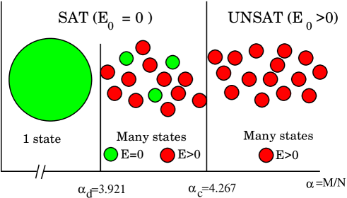
Figure 1: A pictorial description of the phase diagram for random 3-SAT obtained in the cavity method: clusters of SAT (in green/light gray) or UNSAT (in red/dark grey) configurations. One finds three qualitatively different phases, the EASY-SAT phase for $\alpha<\alpha_{d}$, the HARD-SAT phase for $\alpha_{d}<\alpha<\alpha_{c}$, the UNSAT phase obtained for $\alpha_{c}<\alpha$ (see text)

The analytic study of MEPAZE ; MZ_pre for the random 3-SAT problem at zero temperature shows the following phase diagram (see fig.1):

• For $\alpha<\alpha_{d}=3.921$, the problem is generically SAT; the solution can be found relatively easily, because the space of SAT configurations builds up a single big connected cluster. A $T=0$ Metropolis algorithm, in which one proposes to flip a randomly chosen variable, and accepts the change iff the number of violated constraints in the new configuration is less or equal to the old one, is able to find a SAT configuration. We call this the EASY-SAT phase

• For $\alpha_{d}<\alpha<\alpha_{c}=4.267$, the problem is still generically SAT, but now it becomes very difficult to find a solution (we call this the HARD-SAT phase). The reason is that the configurations of variables which satisfy all constraints build up some clusters. Each such cluster, which we call a ’state’, is well separated from the other clusters (passing from one to the other requires flipping an extensive number of variables). But there also exist many “metastable states”: starting from a random configuration, a local descent algorithm will get trapped in some cluster of configurations with a given finite energy (they all have the same number of violated clauses, and it is impossible to get out of this cluster towards lower energy configurations through any descending sequence of one spin flip moves). The number of SAT clusters ${\cal N}$ is exponentially large in $N$, it behaves as ${\cal N}\sim\exp(N\Sigma)$; but the number of metastable clusters is also exponentially large with a larger growth rate, behaving like $\exp(N\Sigma_{ms})$ with $\Sigma_{ms}>\Sigma$. The most numerous metastable clusters, which have an energy density $e_{th}$, will trap all local descent algorithms (zero temperature Metropolis of course, but also simulated annealing, unless it is run for an exponential time).

• For $\alpha>\alpha_{c}$, the problem is typically UNSAT. The ground state energy density $e_{0}$ is positive. Finding a configuration with lowest energy is also very difficult because of the proliferation of metastable states.

A more quantitative description of the thermodynamic quantities in the various phases is shown in fig.2. The most striking result is the existence of an intermediate SAT phase where clustering occurs. A hint of such a behavior had been first found in a sophisticated variational one step replica symmetry breaking approximation developed in BMW ; however this approximation predicted a second order phase transition (clusters separating continuously), while we now think that the transition is discontinuous: an exponentially large number of macroscopically separated clusters appears discontinuously at $\alpha=\alpha_{d}$. Another point which should be noticed is the fact that the complexity, and the energy $e_{th}$ in the HARD-SAT phase are rather small: around $e_{th}\sim 3\ 10^{-3}$ violated clause per variable for $\alpha=4.2$. This shows that until one reaches problems with at least a few thousands variables, one cannot feel the true complexity of the problem. This can explain why the existence of the intermediate phase went unnoticed in previous simulations.

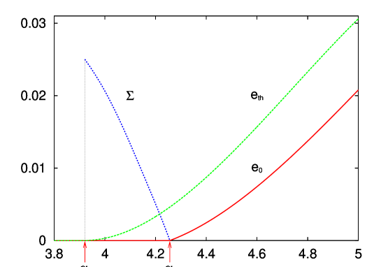
Figure 2: Thermodynamic quantities for the random 3-SAT problem: $e_{0}$ is the ground state energy density (minimal number of violated clauses per variable); $e_{th}$ is the energy density of the most numerous metastable states,which trap the local descent algorithms; $\Sigma$ is the complexity of SAT states with $E=0$

The second type of results found in MEPAZE ; MZ_pre ; BMZ is a new class of algorithms dealing with the many states structure. Basically this algorithm amounts to using the cavity equations on one given sample. Originally the cavity method was developed to handle a statistical distribution of samples. For instance in the random 3-SAT case its basic strategy is to add one extra variable and connect it randomly to a number of new clauses which has the correct statistical distribution. In the large $N$ limit, the statistics of the local field on the new variable should be identical to the statistics of the local fields on any other variable in the absence of the new one. It turns out that this strategy can be adapted to study a single sample: one considers a given clause $a$, which involves three variables $\sigma_{1},\sigma_{2},\sigma_{3}$. The cavity field on $\sigma_{1}$ is the field felt by $\sigma_{1}$ in the absence of $a$. In the case where there exist many states, there is one such field for each possible state of the system, and the order parameter is the survey of these fields, in all the states of fixed energy density $e$:

$$P_{0}^{e}(h)=C^{t}\sum_{\alpha}\delta\left(h_{0}^{\alpha}-h\right)\delta\left(\frac{E^{\alpha}}{N}-e\right)$$ (3)

One can then write a recursion recursion between these surveys. Looking for instance at the structure of fig.3, one gets the following iteration equation:

$$P_{0}^{e}(h) = C^{t}\int P_{\sigma_{1}}^{e}(g_{1})dg_{1}\;P_{\tau_{1}}^{e}(h_{1})dh_{1}\;P_{\sigma_{2}}^{e}(g_{2})dg_{2}\;P_{\tau_{2}}^{e}(h_{2})dh_{2}$$ (4)

$$\delta(h-f(g_{1},h_{1},g_{2},h_{2}))\exp\left(-\frac{d\Sigma}{de}w(g_{1},h_{1},g_{2},h_{2})\right)$$

The function $f$ just computes the value of the new cavity field on $\sigma_{0}$ in terms of the four cavity fields $g_{1},h_{1},g_{2},h_{2}$. It is easily computed by considering the statistical mechanics problem of the five-spin system $\{\sigma_{0},\sigma_{1},\tau_{1},\sigma_{2},\tau_{2}\}$ and summing over the 16 possible states of the spins $\sigma_{1},\tau_{1},\sigma_{2},\tau_{2}$. The function $w$ computes the free energy shift induced by the addition of $\sigma_{0}$ to the system with the four spins $\sigma_{1},\tau_{1},\sigma_{2},\tau_{2}$. The exponential reweighting term in (4) is the crucial piece of survey propagation: it appears because one considers the survey at a fixed energy density $e$. As the number of states at energy $E=Ne+\delta E$ increases in $\exp(y\delta E)$, where $y=\frac{d\Sigma}{de}$, this favors the states with a large negative energy shift.

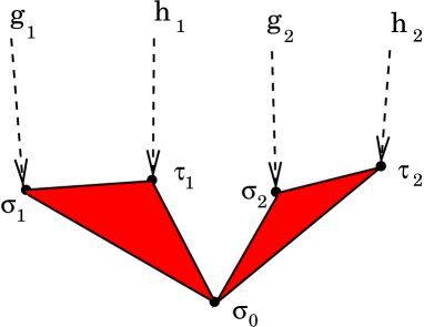
Figure 3: The basic iterative structure of survey propagation. This subgraph is a part of a 3-SAT problem, in which the variable $\sigma_{0}$ belongs to three 3-clauses, involving respectively the variables $\{\sigma_{1},\tau_{1}\},\{\sigma_{2},\tau_{2}\},\{\sigma_{3},\tau_{3}\}$. When the clause 3 is switched off, the local cavity field survey $P_{0}^{e}(h)$ on spin $\sigma_{0}$ can be computed in terms of the cavity field surveys on each of the spins $\sigma_{1},\tau_{1},\sigma_{2},\tau_{2}$.

The usual cavity method for the random 3-SAT problem determines the probability, when a new variable is added at random, that its survey $P_{0}^{e}(h)$ is a given function $P(h)$: the order parameter is thus a functional, the probability of a probability. Because the fields are distributed on integers, this object is not as terrible as it may look and it is possible to solve the equation and compute the ’complexity curve’ $\Sigma(E)$, giving the phase diagram described above.

The algorithm for one given sample basically iterates the survey propagation equation on one given graph. It is a message passing algorithm which can be seen as a generalization of the belief propagation algorithm familiar to computer scientistspearl . The belief propagation is a propagation of local magnetic fields, which is equivalent to using a Bethe approximation yed . Unfortunately, it does not converge in the hard-SAT region because various subparts of the graph tend to settle in distinct states, and there is no way to globally choose a state. In this region, the survey propagation, which propagates the information on the whole set of states (in the form of a histogram), does converge.

Based on the surveys, one can detect some strongly biased spins, which are fixed to one in almost all SAT configurations. The “Survey Inspired Decimation” (SID) algorithm fixes the spin which is most biased, then it re-runs the survey propagation on the smaller sample so obtained, and then iterates… An example of the evolution of the complexity as a function of the decimation is shown in 4. This algorithm has been tested in the hard SAT phase. It easily solves the ’large’ benchmarks of random 3sat at $\alpha=4.2$ with $N=1000,2000$ available at SATLIB . It turns out to be able to solve typical random 3-SAT problems with up to $N=10^{7}$ at $\alpha=4.2$ in a few hours on a PC, which makes it much better than available algorithms. The main point is that the set of surveys contains a lot of detailed information on a given sample and can probably be used to find many new algorithms, of which SID is one example.

Figure 4: The total complexity (= the $\ln$ of the number of states) as a function of the total energy (= the number of violated clauses) for one given sample with $N=10^{4}$ variables and $M=4.2\;10^{4}$ constraints. The top curve is the original complexity. The next curves are the various complexities obtained for the decimated samples, plotted here every $200$ decimations. One sees a global decrease of the number of metastable states, and also a global decrease of the threshold energy. In the end the problem has no more metastable states and can be solved by simple algorithms.

To summarize, the recent statistical physics approaches to the random 3-SAT problem give the following results:

• An analytic result for the phase diagram of the generic samples

• An explanation for the slowdown of algorithms near $\alpha_{c}=4.267$: this is due to the existence of a HARD-SAT phase at $\alpha\in[3.921,4.267]$, with exponentially many metastable states.

• An algorithm for single sample analysisweb : Survey propagation converges and yields very non trivial information on the sample. It can be used for instance to decimate the problem and get an efficient SAT-solver in the hard-SAT region.

This whole set of results calls for a lot of developments in many directions.

On the analytical side, the cavity method results quoted above are believed to be correct, but they are not proven rigorously. It would be very interesting to turn these computations into a rigorous proof. A very interesting step in this direction was taken recently by Franz and Leone who showed that the result for the critical threshold $\alpha_{c}$ obtained by the cavity method on random K-SAT with $K$ even actually give a rigorous upper bound to the critical $\alpha_{c}$ FraLeo . The whole construction of the cavity method with the clustering structure, the many states and the resulting reweighting, has actually been checked versus rigorous computations on a variant of the SAT problem, the random XORSAT problem, where rigorous computations xorsat have confirmed the validity of the approach.

On the numerical side, one needs to develop convergence proofs for survey propagation, and to derive the generalization of the algorithm for the case in which there exists local structures in the interaction graphs. This will amount to generalizing from a Bethe like approximation (with many states) to a cluster variational method with larger clusters (and with many states).

The techniques can also be extended to other optimization problems like coloring colouring . Beside the problems mentioned here, there exist many other fascinating problems of joint interests to physicists and computer scientists, like e.g the dynamical behavior of algorithms in optimization or error correcting codes, which I cannot survey here. Let me just quote a few recent references to help the readers through the corresponding bibliography cocmon ; global_algorithm ; FLMR ; MonZec .

Acknowledgements It is a pleasure to thank all my collaborators over the years on various topics at the interface between statistical physics and optimization. I am particularly thankful to G. Parisi and R. Zecchina for the wonderful collaborations over the last three years which lead to the works on the cavity method and the satisfiability problem.

References

- (1) C.H. Papadimitriou and K. Steiglitz, Combinatorial Optimization, Dover (Mineola, N.Y., 1998).
- (2) Mézard, M., Parisi, G., Virasoro, M.A. Spin Glass Theory and Beyond, World Scientific, Singapore (1987).
- (3) Kirkpatrick, S., Gelatt Jr., C. D. Vecchi, M. P. Optimization by simulated annealing, Science 220 671–680(1983). Černy, V., Thermodynamical approach to the traveling salesman problem: An efficient simulation algorithm, J. Optimization Theory Appl.45 41 (1985).
- (4) See e.g. A. Montanari, The glassy phase of Gallager codes cond-mat/0104079, and references therein.
- (5) Dubois O. , Monasson R., Selman B. Zecchina R. (Eds.), Phase Transitions in Combinatorial Problems, Theoret. Comp. Sci. 265 (2001).
- (6) C.H. Papadimitriou, Computational complexity (Addison-Wesley, 1994)
- (7) Cook, S. The complexity of theorem–proving procedures, in: Proc. 3rd Ann. ACM Symp. on Theory of Computing, Assoc. Comput. Mach., New York, 1971, p. 151.
- (8) Levin L.A., Average case complete problems, SIAM J. Comput., 14 (1): 285-286 (1986); Ben-David S., Chor B., Goldreich O. Luby M., On the theory of average case complexity, JCSS 44, 193-219; Gurevich Y., Average Case completeness, JCSS 42, 246-398 (1991).
- (9) , M. Mézard and J. Vannimenus, On the statistical mechanics of optimization problems of the traveling salesman type, J. Physique Lett. 45 (1984) L1145.
- (10) M. Mézard and G. Parisi, Replicas and Optimization, J.Phys.Lett. 46 (1985) L771.
- (11) D. Aldous, The zeta(2) Limit in the Random Assignment Problem, Random Structures and Algorithms 18 (2001) 381-418.
- (12) Fu Y. and Anderson P. W., Application of Statistical Mechanics to NP-Complete Problems in Combinatorial Optimization, J. Phys. A 19, 1605–1620 (1986).
- (13) A nice pedagogical introduction is B. Hayes I can’t get no satisfacion, American Scientist 85 (1997) 108.
- (14) S. Kirkpatrick, B. Selman, Critical Behaviour in the satisfiability of random Boolean expressions, Science 264, 1297 (1994)
- (15) Crawford J.A. Auton L.D., Experimental results on the cross-over point in random 3-SAT, Artif. Intell. 81, 31-57 (1996).
- (16) R. Monasson, R. Zecchina, S. Kirkpatrick, B. Selman and L. Troyansky, Nature (London) 400, 133 (1999).
- (17) A. Kaporis, L. Kirousis, E. Lalas, The probabilistic analysis of a greedy satisfiability algorithm, in Proceedings of the 4th European Symposium on Algorithms (ESA 2002), to appear in series: Lecture Notes in Computer Science, Springer;
- (18) D. Achlioptas, G. Sorkin, 41st Annu. Symp. of Foundations of Computer Science, IEEE Computer Soc. Press, 590 (Los Alamitos, CA, 2000).
- (19) J. Franco, Results related to threshold phenomena research in satisfiability: lower bounds, Theoretical Computer Science 265, 147 (2001)
- (20) O. Dubois, Y. Boufkhad, J. Mandler, Typical random 3-SAT formulae and the satisfiability threshold, in Proc. 11th ACM-SIAM Symp. on Discrete Algorithms, 124 (San Francisco, CA, 2000).
- (21) Monasson, R. Zecchina, R. Entropy of the K-satisfiability problem, Phys. Rev. Lett. 76 3881–3885(1996).
- (22) Monasson, R. Zecchina, R., Statistical mechanics of the random K-Sat problem, Phys. Rev. E 56 1357–1361 (1997).
- (23) Biroli, G., Monasson, R. Weigt, M. A Variational description of the ground state structure in random satisfiability problems, Euro. Phys. J. B 14 551 (2000).
- (24) S. Franz, M. Leone, F. Ricci-Tersenghi, R. Zecchina, Exact Solutions for Diluted Spin Glasses and Optimization Problems, Phys. Rev. Lett. 87, 127209 (2001).
- (25) M. Mézard, G. Parisi and R. Zecchina, Science 297, 812 (2002) (Sciencexpress published on-line 27-June-2002; 10.1126/science.1073287)
- (26) Random 3-SAT: from an analytic solution to a new efficient algorithm, M. Mézard and R. Zecchina, Phys.Rev. E 66 (2002) 056126.
- (27) Survey propagation: an algorithm for satisfiability, A. Braunstein, M. Mézard, R. Zecchina, http://fr.arXiv.org/abs/cs.CC/0212002.
- (28) Mézard, M. Parisi, G. The Bethe lattice spin glass revisited. Eur.Phys. J. B 20, 217–233 (2001). Mézard, M. Parisi, G. The cavity method at zero temperature, J. Stat. Phys. in press.
- (29) J. Pearl, Probabilistic Reasoning in Intelligent Systems, 2nd ed. (San Francisco, MorganKaufmann,1988).
- (30) J.S. Yedidia, W.T. Freeman and Y. Weiss, Generalized Belief Propagation, in Advances in Neural Information Processing Systems 13 eds. T.K. Leen, T.G. Dietterich, and V. Tresp, MIT Press 2001, pp. 689-695.
- (31) Satisfiability Library: www.satlib.org/
- (32) S. Franz and M. Leone, Replica bounds for optimization problems and diluted spin systems, preprint cond-mat/0208280, available at http://fr.arXiv.org
- (33) M. Mézard, F. Ricci-Tersenghi, R. Zecchina, Alternative solutions to diluted p-spin models and XOR-SAT problems, cond-mat/0207140, (2002). S. Cocco, O. Dubois, J. Mandler, R. Monasson, Rigorous decimation-based construction of ground pure states for spin glass models on random lattices, cond-mat/0206239 (2002).
- (34) Coloring random graphs, R. Mulet, A. Pagnani, M. Weigt, R. Zecchina, cond-mat/0208460.
- (35) Restart method and exponential acceleration of random 3-SAT instances resolutions: a large deviation analysis of the Davis-Putnam-Loveland-Logemann algorithm, S. Cocco and R. Monasson, cond-mat/0206242
- (36) Complexity transitions in global algorithms for sparse linear systems over finite fields, J. Phys. A 35, 7559 (2002), A. Braunstein, M. Leone, F. Ricci-Tersenghi, R. Zecchina.
- (37) The Dynamic Phase Transition for Decoding Algorithms, S. Franz, M. Leone, A. Montanari, F. Ricci-Tersenghi, cond-mat/0205051.
- (38) Boosting search by rare events, A. Montanari, R. Zecchina, cond-mat/0112142.
- (39) www.ictp.trieste.it/zecchina/SP