Exact analytic solution for the generalized Lyapunov exponent of the 2-dimensional Anderson localization

Abstract

The Anderson localization problem in one and two dimensions is solved analytically via the calculation of the generalized Lyapunov exponents. This is achieved by making use of signal theory. The phase diagram can be analyzed in this way. In the one dimensional case all states are localized for arbitrarily small disorder in agreement with existing theories. In the two dimensional case for larger energies and large disorder all states are localized but for certain energies and small disorder extended and localized states coexist. The phase of delocalized states is marginally stable. We demonstrate that the metal-insulator transition should be interpreted as a first-order phase transition. Consequences for perturbation approaches, the problem of self-averaging quantities and numerical scaling are discussed.

1 Introduction

Frequently problems arise in science which involve both additive and multiplicative noise. The first type is relatively easy to handle with the help of the central limit theorem. The situation changes dramatically with the appearance of multiplicative noise. Famous examples are the Anderson localization, turbulence, and the kicked quantum rotator among others. In this field results of an importance comparable to the central limit theorem are still lacking. Moreover, the approaches are in general numerical ones and analytical tools are the rare exception.

We present such an analytic approach which permits to deal in great generality with processes involving multiplicative and additive noise even in the limit of strong disorder. In this paper we apply the formalism to the famous Anderson localization in a two-dimensional (2-D) disordered system which is one of the paradigms of solid state theory.

The quantum mechanical consequences of disorder in solids have first been revealed by Anderson [1]. The Anderson model provides a standard framework for discussing the electronic properties of disordered systems, see reviews [2, 3, 4]. The nature of electronic states in the Anderson model depends strongly on the spatial dimension $D$. It has been shown rigorously that in one dimension (1-D) all states are localized at any level of disorder [3, 5]. The shape of these localized wave functions is characterized by an asymptotic exponential decay described by the Lyapunov exponent $\gamma$. The most important results for dimensions higher than one follow from the famous scaling theory of localization [6, 7], which assumes a single scaling parameter for the dimensionless conductance $g$ or, equivalently, the localization length $\xi=1/\gamma$. The conclusion of the scaling theory is that for $D\leq 2$ all states are localized at any level of disorder, while a delocalization (metal-insulator) transition occurs for $D>2$ if the disorder is sufficiently strong. A detailed review of the scaling theory for disordered systems can be found in [2, 4].

The 2-D case still presents a problem, since there is no exact analytical solution to the Anderson problem, and all numerical results published so far rely on finite-size scaling [3, 8]. Recent studies [9] have questioned the validity of the single parameter scaling theory, including the existence of a finite asymptotic localization length for $D=2$. Additional boost of interest in the $2D$ Anderson model has been triggered by experimental observations of Kravchenko et al. [10, 11] of a metal-insulator transition in thin semiconductor films, which contradicts the conventional scaling theory. Moreover, recent experiments of Ilani et al. [12, 13] can be interpreted in terms of the coexistence of localized and delocalized states. These experiments are still being discussed controversially. The experimental reality is certainly more complex than the simple tight-binding schemes used in the theoretical treatment so far and in particular the electronic iteractions could play a role in the above mentioned experimental situations. But nevertheless these results add doubts to the status of the localization theory in 2-D. Before embarking on computational schemes beyond the tight-binding approach, which necessarily lead to more restricted system sizes and other approximations, it appears advisable to try to solve as rigourously as possible the problem in the tight-binding scheme. In the present controversial situation the first step in resolving the conflict is thus in our opinion to consider exact results that do not rely on the scaling theory or small parameter expansions.

The starting point for the method presented in this paper is found in the work of Molinari [14], in which the Anderson problem for the 1-D system is dealt with as a statistical stability problem for the solutions $\psi_{n}$ of the tight binding Hamiltonian in a semi-infinite system, $n\geq 0$. It was shown in ref. [14] that the equations for the statistical moments of the type $\langle\psi^{2j}_{n}\rangle$ can be obtained analytically (explicit solutions are given for $j=1,2$), which enabled the author to derive exact generalized Lyapunov exponents. We will show in the following that this approach can be further generalized for systems of higher spatial dimensions. But it turns out to be unavoidable to change again the mathematical tools for the treatment. In the present investigation we use both for the 1-D and the 2-D case the tool of signal theory abundantly used in electrical engineering, see e.g.[15]. The basic idea in applying signal theory to the problem of Anderson localization is to interpret certain moments of the wave function as signals. There is then in signal theory a qualitative difference between localized and extended states: The first ones correspond to unbounded signals and the latter ones to bounded signals. In the case of a metal-insulator transition extended states (bounded signals) transform into localized states (unbounded signals). Signal theory shows that it is possible in this case to find a function (the system function or filter), which is responsible for this transformation. The advantage of working with filters instead of the signals themselves lies in the fact that the filters do not depend on initial conditions in contrast to the signals. The existence of this transformation in a certain region of disorder and energy simply means that the filter looses its stability in this region. The meaning of an unstable filter is defined by a specific pole diagram in the complex plane. These poles also define a quantitative measure of localization. Thus it is possible here to determine the socalled generalized Lyapunov exponents as a function of disorder and energy.

The outline of the present article is as follows. In chapter 2 we treat the 1-D case in detail describing also essential elements of signal theory. The theory for the 2-D problem is presented in chapter 3 and the results are given in chapter 4. In the latter chapter also the implications of the present approach for perturbation theory, the order of the phase transition and the problem of self-averaging is discussed as well as numerical scaling.

2 1-D case

2.1 Recursion relation

We start for pedagogical and methodical reasons with the treatment of the 1-D case. The aim of this section is to apply mathematical tools which are new in the field of Anderson localization but well-known from other fields and which may and do in fact prove useful also for the higher dimensional cases.

We start from the Hamiltonian of the standard 1-D Anderson model in the tight-binding representation

$$\mathcal{H}=\sum_{n}\varepsilon_{n}|n\rangle\langle n|+t\sum_{n}\left[|n\rangle\langle n+1|+|n\rangle\langle n-1|\right],$$ (1)

where $t$ is the hopping matrix element (units with t=1 are used below) and the $\varepsilon_{n}$ are the on-site potentials which are random variables to simulate the disorder. The $\varepsilon_{n}$ are independently and identically distributed with existing first two moments, $\left\langle\varepsilon_{n}\right\rangle=0$ and $\left\langle\varepsilon_{n}^{2}\right\rangle=\sigma^{2}$. This model is well investigated [3, 5, 16] and it is known that for any degree of disorder the eigenfunctions become localized. This in turn means that $|\psi_{n}|^{\delta}$ with $\delta>0$ is growing exponentially in the mean on a semi-infinite chain where the rate of growth is described by the Lyapunov exponent.

In the one-dimensional case one can compute the Lyapunov exponent by different methods and under different assumptions [17] or numerically by means of the transfer matrix method which results in solving a recurrence equation [18]. The disadvantage of these analytical methods is that they cannot be easily extended to the 2-D and 3-D cases. In this paper we want to show that one can construct an approach which is able to handle all cases from a universal point of view.

It is well-known that the two-point boundary problem for a finite difference analog to the stationary Schrödinger equation with homogeneous boundary conditions can be reduced to a Cauchy problem with the one-side (initial) condition [19]

$$\psi_{0}=0,\psi_{1}=\alpha.$$ (2)

Due to the linearity of the equation the non-zero value of $\alpha$ serves only as a normalization parameter. The asymptotic behaviour of the solution is completely determined by the energy $E$ and the level of disorder $\sigma$. The presence of a boundary permits one to rewrite the Schrödinger equation

$$\psi_{n+1}+\psi_{n-1}=(E-\varepsilon_{n})\psi_{n}$$ (3)

in the form of a recursion relation for the grid amplitude of the wave function $\{\psi_{n}\}$ ($n=1,2,\ldots$):

$$\psi_{n+1}=(E-\varepsilon_{n})\psi_{n}-\psi_{n-1}.$$ (4)

Statistical correlations in this equation are separated: it is easy to see that in a formal solution of the recursion relation the amplitude $\psi_{n+1}$ depends only on the random variables $\varepsilon_{n^{\prime}}$ with $n^{\prime}\leq n$, which is the causality principle. This observation has been extensively used by Molinari[14] in the solution for the 1-D case. We emphasize that this property is fundamental as a key for obtaining an exact solution to the Anderson problem for all dimensions. Note that both amplitudes $\psi_{n}$ and $\psi_{n-1}$ on the r.h.s. of eq. (4) are statistically independent of $\varepsilon_{n}$.

The equation for the first moment of the random variable $\psi_{n}$ does not include the parameter $\sigma$:

$$\left\langle\psi_{n+1}\right\rangle=E\left\langle\psi_{n}\right\rangle-\left\langle\psi_{n-1}\right\rangle.$$ (5)

The ansatz $\left\langle\psi_{n}\right\rangle=\lambda^{n}$ results in the $\lambda_{1,2}$ which satisfy the equation $\lambda+{\lambda}^{-1}=E$. Energies with $|E|<2$, where $|\lambda_{1,2}|=1$ and $\lim_{n\to\infty}\langle\psi_{n}\rangle<\infty$, obviously coincide with the band of delocalized states in a perfect chain ($\sigma=0$).

2.2 Lyapunov exponents as order parameter

A bounded asymptotical behaviour of the first moment at any level of disorder indicates that there are always physical solutions inside the band $|E|<2$. Further information about the character of these states (localized / delocalized) can be gained by considering the other moments. For one-dimensional models with random potential the eigenstates are always exponentially localized [5]. The natural quantities to investigate is therefore the Lyapunov exponent $\gamma_{0}$

$$\gamma_{0}=\lim_{n\rightarrow\infty}\frac{1}{n}\left\langle\ln|\psi_{n}|\right\rangle$$ (6)

or its generalization [14, 18]

$$\gamma_{\delta}=\lim_{n\rightarrow\infty}\frac{1}{n\delta}\ln\left\langle|\psi_{n}|^{\delta}\right\rangle.$$ (7)

The generalized exponents have been studied extensively by Pendry et al. (see ref. [18] and references given there), in a systematic approach based on the symmetric group. The method involves the construction of a generalized transfer matrix by means of direct products of the transfer matrices, followed by a reduction of the matrix size. This generalized transfer matrix produces the average values of the required power of the quantity under consideration.

The concept of Lyapunov exponent $\gamma$ and the corresponding localization length $\xi$ describe a statistical stability of solutions of the tight-binding equations. Anderson localization as a metal-insulator transition is a typical critical phenomenon. To determine the phase-diagram of the system we need only make use of the qualitative aspect of the Lyapunov exponent. Two phases differ qualitatively: $\gamma\equiv 0$ for conducting states (metallic phase) and $\gamma\neq 0$ for localized states (insulating phase).

The Lyapunov exponent $\gamma$ is a typical order parameter [20]. It is useful to check whether this kind of relation is valid for other systems like ferromagnets and ferroelectrics too. Here the order parameters are the magnetization $M$ and the polarization $P$, respectively. At high temperatures and zero external field these values are $M,P\equiv 0$ (paramagnetic or paraelectric phase). At lower temperatures, however, spontaneous magnetization and polarization arise, $M,P\neq 0$. The order parameter is zero for one phase and becomes nonzero for the other phase. It is well-known that there is no unambiguous definition of an order parameter [20]. This holds also in our case, many different definitions are possible (see e.g. ref. [14] and literature cited there). Every exact Lyapunov exponent either via the log-definition ($\gamma_{0}$) or via the $\delta$-definition ($\gamma_{\delta}$) gives this property. This permits us to consider a transition from the quality $\gamma\equiv 0$ to the quality $\gamma\neq 0$ as a critical point, where all moments $\left\langle|\psi_{n}|^{\delta}\right\rangle$ diverge for $n\rightarrow\infty$ simultaneously. If on the other hand we are interested in the values themselves of the Lyapunov exponents $\gamma\neq 0$, they always depend on the definition. If one prefers a particular definition, this can only be by agreement and always remains quite arbitrary.

In the 1-D case we find the metallic phase ($\gamma=0$) only for $\sigma=0$; even for infinitesimally small disorder one has $\gamma\neq 0$ and only the insulating phase exists. The critical point is therefore $\sigma=\sigma_{0}=0$ independently of the value of the energy $E$, and the phase-diagram is trivial. This situation is typical for a critical phenomenon in a 1-D system with short range interaction [20]: all 1-D systems (e.g. 1-D Ising-model) do not possess a true phase transition at a finite value of the parameter (temperature in the Ising model or disorder $\sigma$ in the Anderson model); one of the phases exists only at a point. One also says [20], that 1-D systems do not possess a phase transition.

The advantage of the new $\delta$-definition rests in the possibility to play with the parameter $\delta$ which gives a new degree of freedom. In quantum theory there are many examples, where a problem is insoluble in the Schrödinger picture, but looks rather simple in the Heisenberg picture. The same holds for representations in coordinate or momentum space. It is always useful to transform the mathematics in such a way that the problem becomes soluble. And nothing else is done here. For $\gamma_{0}$ (log-definition) the problem remains analytically insoluble. Molinari [14] was the first to show that with a generalisation of the definition, and for special values of $\delta=2,4,...$, a simple analytical (algebraic) investigation becomes possible.

Molinari[14] has not only considered a standard definition via ”the log of the wave function” i.e. $\gamma_{0}$, but also a set of so-called generalized Lyapunov exponents $\gamma_{2j}$, $j=1,2,...$ ($\gamma_{2}$ for the square of the wave function). In general all the $\gamma_{2j}$ are quite different parameters. However, it is important that a transition from the quality $\gamma\equiv 0$ to the quality $\gamma\neq 0$ is simultaneous, all $\gamma_{2j}\equiv 0$ for $\sigma=0$ and $\gamma_{2j}\neq 0$ for a disordered system. As has already been established [3, 17], in the limit of small disorder different definitions of the Lyapunov exponent or localization length give values differing only by an integer factor. This property is again a signature for a critical phenomenon. In the vicinity of the critical point $\sigma=\sigma_{0}=0$ as common for all critical phenomena and only one scale dominates. Thus Molinari has shown that for the 1-D Anderson problem all $\gamma_{2j}\approx(1+j)\gamma_{0}$ for $\sigma\rightarrow 0$ (this is proven for $j=1,2,3$), where $\gamma_{0}=\sigma^{2}/2(4-E^{2})$ is taken from other investigations[3, 17, 19], the only difference being the numerical cofactor.

This means that even in 1-D there are other quantities besides the logarithm of the wave function which can be used for the analysis.

2.3 Equations for second moments

In order to obtain the phase diagram it is (based on the above discussion) sufficient to choose a particular and convenient value of the parameter $\delta$, e.g. $\delta=2$, the second moments.

It is shown in ref. [14] that the calculation of the higher moments, $\langle\psi^{2j}_{n}\rangle$ with $j>1$, is important for determining the shape of the distribution of $|\psi_{n}|$, but at the same time the higher moments of the on-site potentials beyond the second one must be considered. We will restrict ourselves here to the pair moments only. Then the initial full stochastic problem eq. (4) can be mapped onto an exactly solvable algebraic problem, in which the random potentials are characterized by a single parameter $\sigma$.

Two points should be mentioned: (i) We are at present not interested in the shape of the distribution which is influenced by the higher moments of the on-site potentials but in the problem of localization (phase-diagram); (ii) In the analysis of the moments of the amplitudes the localization of states finds its expression in the simultaneous divergence of the even moments for $n\rightarrow\infty$. Because the second moment depends only on the parameter $\sigma$ this means that the critical properties are completely determined by $\sigma$.

We are interested in the mean behavior of $\psi^{2}_{n}$ which follows from eq. (4) as:

$$\langle\psi_{n+1}^{2}\rangle=\langle[(E-\epsilon_{n})\psi_{n}-\psi_{n-1}]^{2}\rangle$$

$$=(E^{2}+\sigma^{2})\langle\psi_{n}^{2}\rangle-2E\langle\psi_{n}\psi_{n-1}\rangle+\langle\psi_{n-1}^{2}\rangle.$$ (8)

In the derivation of eq. (2.3) the mean of the product of uncorrelated quantities was replaced by the product of the means. The resulting equation is open ended, but the new type of the means $\langle\psi_{n}\psi_{n-1}\rangle$ can be easily calculated:

$$\langle\psi_{n}\psi_{n-1}\rangle = \langle[(E-\epsilon_{n-1})\psi_{n-1}-\psi_{n-2}]\psi_{n-1}\rangle$$ (9)

$$= E\langle\psi_{n-1}^{2}\rangle-\langle\psi_{n-1}\psi_{n-2}\rangle.$$

Let us rewrite these equations using $x_{n}=\langle\psi^{2}_{n}\rangle$ and $y_{n}=\langle\psi_{n}\psi_{n-1}\rangle$:

$$x_{n+1} = (E^{2}+\sigma^{2})\,x_{n}-2Ey_{n}+x_{n-1},$$ (10)

$$y_{n} = E\,x_{n-1}-y_{n-1}.$$ (11)

The initial conditions are:

$$x_{0}=0,x_{1}=\alpha^{2},y_{0}=0.$$ (12)

Let us summarize the intermediate results up to this point. The causality principle has led to a set of linear algebraic equations for the second moments of the random field instead of an infinite hierarchy of equations that couple the second moments with the third ones etc. The set of equations is closed, but it does not include all possible second moments of the type $\langle\psi_{n}\psi_{n^{\prime}}\rangle$ (this fact is irrelevant in the search for localization criteria). At this level the on-site potentials are also characterized by a single second moment $\sigma^{2}$ only, which implies that the shape of the distribution does not matter for localization. Information on higher moments is a crucial step for other models, e.g., in turbulence and econophysics because the third and the fourth moments are linked to skewness and kurtosis of the distribution which are interesting features in these fields. Equations for the higher moments can be easily constructed using the same causality property[14], but in the treatment of the Anderson problem we restrict ourselves to the second moment only. The set of equations is exact in the sense that no additional approximations were made in its derivation. Therefore, we conclude that at the given point the stochastic part of the solution to the Anderson problem is completed and one has to deal further only with a purely algebraic problem.

The set of equations (10), (11) can be solved by different methods of linear algebra.

2.4 Transfer matrix

We employ first a simple matrix technique. The eqs. (10), (11) can be rewritten in the form

$$w_{n+1}=T\,w_{n}\,,$$ (13)

where the vector $w_{n}$ and the transfer matrix $T$ are respectively

$$w_{n}=\left(\begin{array}[]{c}x_{n+1}\\ x_{n}\\ y_{n+1}\end{array}\right)\,,\,T=\left(\begin{array}[]{ccc}E^{2}+\sigma^{2}&1&-2E\\ 1&0&0\\ E&0&-1\end{array}\right)\,.$$ (14)

Initial conditions transform into $w_{0}=\{\alpha^{2},0,0\}$.

An explicit formula for $w_{n}$ is derived by diagonalizing the transfer matrix $T$. The characteristic equation of the eigenvalue problem for the $T$ matrix is

$$\mathcal{D}(\lambda)=0$$ (15)

with function $\mathcal{D}(z)=z^{3}-(E^{2}+\sigma^{2}-1)z^{2}+(E^{2}-\sigma^{2}-1)z-1$.

The solution of the cubic characteristic equation (15) can be given explicitly in radicals (Cardan’s formula). Corresponding expressions are known and not presented here. It is significant that one of the eigenvalues (let it be $\lambda_{1}$) is always real and $\lambda_{1}\geq 1$. Other solutions, $\lambda_{2}$ and $\lambda_{3}$, are either complex conjugate to each other or both real and satisfy $|\lambda_{2,3}|\leq 1$. These properties result from the fact that the coefficients $E^{2}$ and $\sigma^{2}$ are non-negative.

The solution of eq. (13) reads as follows:

$$w_{n} = U\cdot\Lambda(n)\cdot U^{-1}w_{0},$$ (16)

where $\Lambda(n)$ is a diagonal matrix containing the n-th power of $\lambda_{i}$ and $U$ is the eigenvector matrix. The resulting exact formula for $x_{n}$ is

$$x_{n}/\alpha^{2} = \frac{\lambda_{1}^{n}(1+\lambda_{1})}{(\lambda_{2}-\lambda_{1})(\lambda_{3}-\lambda_{1})}+$$

$$+ \frac{\lambda_{2}^{n}(1+\lambda_{2})}{(\lambda_{1}-\lambda_{2})(\lambda_{3}-\lambda_{2})}+$$

$$+ \frac{\lambda_{3}^{n}(1+\lambda_{3})}{(\lambda_{1}-\lambda_{3})(\lambda_{2}-\lambda_{3})}\,.$$

Thus we have the full algebraic solution for any energy $E$ and any degree of disorder $\sigma$. From the functional form of the eq. (2.4) one can see that the roots of eq. (15), $\lambda_{i}$, give us the Lyapunov exponents $\gamma$ of the problem, $\lambda=\exp(2\gamma)$, so the judgement on a localization transition can be done immediately after arriving at eq. (15). Electronic states satisfying the inequality $\max|\lambda_{i}|=\lambda_{1}>1$ correspond to localization.

2.5 Z-transform

An alternative solution makes use of the so-called Z-transform. This is used mainly in Electrical Engineering for discrete-time systems and we suggest as publicly available source [15]. The Z-transform of the quantities $x_{n}$ and $y_{n}$ to functions $X(z)$ , $Y(z)$ is defined by

$$X(z)=\sum_{n=0}^{\infty}\frac{x_{n}}{z^{n}},Y(z)=\sum_{n=0}^{\infty}\frac{y_{n}}{z^{n}}.$$ (18)

The inverse Z-transform is quite generally defined via countour integrals in the complex plane

$$x_{n}=\frac{1}{2\pi i}\oint X(z)z^{n}\frac{dz}{z}.$$ (19)

We further on need the following properties: for the Z-transform

$$x_{n+n_{0}}\Rightarrow z^{n_{0}}X(z),$$ (20)

and for the inverse Z-transform

$$\frac{z}{z-\lambda}\Rightarrow\lambda^{n}.$$ (21)

In this way eqs. (18) and (20) translate eqs. (10), (11) into a system of two coupled linear equations for the two unknowns $X$ and $Y$

$$zX = (E^{2}+\sigma^{2})X-2EY+z^{-1}X+\alpha^{2}$$ (22)

$$Y = Ez^{-1}X-z^{-1}Y$$ (23)

This is easily solved for $X(z)$

$$X(z)=\frac{\alpha^{2}z(z+1)}{\mathcal{D}(z)}$$ (24)

where the function $\mathcal{D}(z)$ is defined above. The inverse Z-transform gives us again eq.(2.4). It is easy to see that the solution of the characteristic equation (15) for the transfer matrix is equivalent to the determination of the poles of the $X(z)$ function. The eigenvalues $\lambda_{i}$, i.e. the poles, determine according to eq. (21) the asymptotic behaviour of the solution $x_{n}$ for $n\rightarrow\infty$. (This is a simplified example for the general relation).

2.6 Signal Theory

Let us start with the following definitions. Let

$$X^{(0)}(z)=\alpha^{2}\frac{(z+1)}{(z-1)}\frac{z}{(z+1)^{2}-zE^{2}}$$ (25)

describe an ideal system ($X^{(0)}(z)=X(z)$ for $\sigma\equiv 0$). This function is independent of the parameter $\sigma$. For $\sigma\neq 0$

$$X(z)=H(z)X^{(0)}(z),$$ (26)

with

$$H(z)=\frac{(z-1)[(z+1)^{2}-zE^{2}]}{\mathcal{D}(z)}.$$ (27)

Note that the boundary conditions (parameter $\alpha$) influence only the function $X^{(0)}(z)$. The function $H(z)=1$ for $\sigma=0$.

Eq. (26) possesses quite a remarkable structure which is better interpreted in the context of signal theory [15], which makes intensive use of the Z-transform. Let us define the system input as $X^{(0)}(z)$ (it characterizes the ideal system), the system output as $X(z)$ (the disordered system), then the function $H(z)$ is the system function or filter. The inverse Z-transform gives [15]

$$x_{n}=\sum_{l=0}^{n}x_{l}^{(0)}h_{n-l}.$$ (28)

Signal theory is not very crucial for the $D=1$ case, because the solution, eq.(24), looks very simple and the inverse Z-transform is always possible. For $D>1$, however, the use of signal theory is exceedingly important because the corresponding solution $X(z)$ can be a very complicated function and an inverse transform may be impossible to find. In the present case it is, however, completely sufficient to investigate the analytic properties of the filter function $H(z)$, i.e. the poles $z=\lambda_{i}$, because the poles determine uniquely the properties of the system. The essential idea is very simple. In the band $|E|<2$ all wave amplitudes (and input signals $x_{n}^{(0)}$) are bounded. Output signals $x_{n}$ are unbounded only under the condition that the filter $h_{n}$ is unbounded for $n\rightarrow\infty$. This property depends on the position of the poles $\lambda_{i}$ in the function $H(z)$.

It is known [15] that the filter $H(z)$ can be characterized by a pole-zero diagram which is a plot of the locations of the poles $\lambda_{i}$ and zeros in the complex z-plane. Since the signals $x_{n}^{(0)}$ and $x_{n}$ are real, $H(z)$ will have poles and zeros that are either on the real axis, or come in conjugate pairs. For the inverse Z-transform $H(z)\Rightarrow h_{n}$ one has to know the region of convergence (ROC). As follows from physical reasons we are interested only in causal filters ($h_{n}=0$ for $n<0$) that have always ROCs outside a circle that intersects the pole with $max{|\lambda_{i}}|$. A causal filter is stable (bounded input yields a bounded output) if the unit circle $|z|=1$ is in the ROC.

To give an example. We start the analysis of the solution with the case of the ideal system, $\sigma=0$. All solutions in the band $|E|<2$ (defined as a region with asymptotically finite first moment) are delocalized with $\lambda_{1}=1$, $\lambda_{2,3}=e^{\pm i2\varphi}$, where $\varphi=\arccos(|E|/2)$. The inverse Z-transform gives us $x_{n}=\alpha^{2}\sin^{2}(\varphi n)/\sin^{2}(\varphi)$. In this case the filter $H(z)=1$ and the ROC of this filter is the full commplex z-plane. The ROC includes the unit circle, the filter $H(z)$ is thus stable, which means the delocalization of all states.

For $\sigma\neq 0$ we always have $\lambda_{1}>1$. The ROC corresponds to the region $|z|\geq\lambda_{1}$, and the unit circle $|z|=1$ lies outside the ROC. A filter $H(z)$ is unstable, in other words, this is simply the localization of all states.

3 2-D case

3.1 Recursion relation

Consider a 2-D lattice with one boundary. The layers of this system are enumerated by an index $n=0,1,\ldots$ starting from the boundary, and the position of an arbitrary lattice site in a particular layer is characterized by an integer $m\in(-\infty,+\infty)$. The presence of a boundary permits one to rewrite the Schrödinger equation

$$\psi_{n+1,m}+\psi_{n-1,m}+\psi_{n,m+1}+\psi_{n,m-1}=(E-\varepsilon_{n,m})\psi_{n,m}$$ (29)

in the form of a recursion relation for the grid amplitude of the wave function $\{\psi_{n,m}\}$ ($n=2,3,\ldots$):

$$\psi_{n,m}=-\varepsilon_{n-1,m}\psi_{n-1,m}-\psi_{n-2,m}+\mathcal{L}\psi_{n-1,m}.$$ (30)

For the sake of a compact notation an operator $\mathcal{L}$ is introduced which acts on the index $m$ according to the equation

$$\mathcal{L}\psi_{n,m}=E\psi_{n,m}-\sum_{\mu=\pm 1}\psi_{n,m+\mu}.$$ (31)

The lattice constant and the hopping matrix element are set equal to unity. The on-site potentials $\varepsilon_{n,m}$ are independently and identically distributed with existing first two moments, $\left\langle\varepsilon_{n,m}\right\rangle=0$ and $\left\langle\varepsilon_{n,m}^{2}\right\rangle=\sigma^{2}$. Eq.(30) is solved with an initial condition

$$\psi_{0,m}=0,\psi_{1,m}=\alpha_{m}.$$ (32)

It turns out to be convenient to consider the index $n$ not as a spatial coordinate, but as discrete time. Then eq. (30) describes the time evolution of a $D-1=1$ dimensional system. It is easy to see that in a formal solution of this recursion relation the amplitude $\psi_{n,m}$ depends only on the random variables $\varepsilon_{n^{\prime},m^{\prime}}$ with $n^{\prime}<n$ (causality). We encounter a very important feature in eq. (30): grid amplitudes on the r.h.s. are statistically independent with respect to $\varepsilon_{n,m}$.

3.2 Implications of signal theory

We are going to generalize further the result of ref. [14] that the set of equations for a certain combination of pair moments is self-contained and can be solved analytically.

The divergence of the moments, which is caused by the localization, is the basis for the existence of Lyapunov exponents for the $n$-direction, which is generally a functional $\gamma[\alpha_{m}]$ of the field $\alpha_{m}$. The well-known idea to define the fundamental Lyapunov exponent for the problem of Anderson localization as a minimal one $\gamma=\min\{\gamma[\alpha_{m}]\}$, is an algorithm but not a general definition, because a fundamental quantity is independent of the initial condition. The proper definition is possible in the framework of signal theory [15].

We define the solutions of the equations for the second moments with disorder ($\sigma>0)$ and without it ($\sigma=0$) as $x$ (system output) and $x^{(0)}$ (system input). Because these equations are linear, there exist an abstract linear operator $\hat{h}$ (system function or filter), which transforms one solution into the other one, $x=\hat{h}x^{(0)}$. It is important that the initial conditions $\alpha_{m}$ only determine the signals, the filter on the other hand is a function of the disorder $\sigma$ only. Divergence of the moments (unbounded output for bounded input) simply means that the filter is unstable[15].

This approach utilizing the concept of the system function is a general and abstract description of the problem of localization. Instead of analyzing the signals $x$ which have restricted physical meaning in the present context because of the chosen normalization we study the filter $\hat{h}$ with properties described by generalized Lyapunov exponents. Then e.g. delocalized states (bounded output) are obtained by transforming the physical solutions inside the band $|E|<4$ (bounded input) provided that the filter $\hat{h}$ is stable.

The transformation $x=\hat{h}x^{(0)}$ is not only valid for individual signals, but also for linear combinations of these signals. Let us regard an ensemble of initial conditions in eq. (32) which is obtained by trivial translation in $m$-space, $\alpha^{\prime}_{m}=\alpha_{m+m_{0}}$. Translation generates physically equivalent signals with identical Lyapunov exponents $\gamma[\alpha_{m}]$. A linear combination of these signals also has this same value $\gamma[\alpha_{m}]$. We construct a linear combination from all such signals with equal weights (this corresponds simply to an average $\langle...\rangle_{0}$ over all possible translations $m_{0}\in(-\infty,+\infty)$).

We here start from the basic fact that the determination of the phase-diagram (the fundamental topic of the paper) requires only the Lyapunov exponents. Signals $x$ are only a means to arrive there. Consequently it is possible to make certain operations with the signals, but under the strict condition that these operations have no influence on the Lyapunov exponents $\gamma[\alpha_{m}]$.

Next we define a full averaging over random potentials and over the ensemble of translations in $m$-space. This latter averaging correponds to the construction of the linear combinations discussed above. Full averaging restores the translational invariance along the $m-$axis, which appears e.g. in $m-$independent diagonal elements, $(n,m)=(n^{\prime},m^{\prime})$, in the set of the second moments of the type $\langle\psi_{n^{\prime},m^{\prime}}\psi_{n,m}\rangle$ and $\langle\psi^{2}_{n,m}\rangle=x_{n}$. We further on regard $x_{n}$ as a one-dimensional signal. If we succeed to solve the equations for $x_{n}$ then we also find not only the Lyapunov exponent $\gamma[\alpha_{m}]$ but simultaneously the projection of the abstract operator on the one-dimensional space, $\hat{h}\rightarrow h_{n}$, because for one-dimensional signals the convolution property eq.(28) exists [15]. The filter $h_{n}$ possesses the same fundamental information as the abstract filter $\hat{h}$ and can easily be analyzed, because signal theory provides a definite mathematical language for this aim (see above). We emphasize here that we do not reduce the problem to a one-dimensional one; it remains two-dimensional. This is quite apparent from the equations below which contain two spatial variables, $n$ and $s=m-m^{\prime}$, the distance along the m-axis.

3.3 Second moments

After the full averaging as defined above the moment $\langle\psi_{1,m^{\prime}}\psi_{1,m}\rangle=\langle\alpha_{m^{\prime}}\alpha_{m}\rangle_{0}=\Gamma_{s}$ (where $s={m-m^{\prime}}$) transforms the initial condition by replacing the field $\alpha_{m}$ by its property correlation function $\Gamma_{s}$ (it is assumed that the field itself and its correlation function are finite). The initial condition for $x_{n}$ reads as $x_{0}=0,x_{1}=\Gamma_{0}$.

Non-diagonal elements, $(n,m)\neq(n^{\prime},m^{\prime})$, depend on the difference $s=m-m^{\prime}$. In the following we will need only three types of moments $f_{n,s}^{\nu}$ with $n^{\prime}=n-\nu$, $\nu=0,1,2$. Let us denote them by $a_{n,s}=f_{n,s}^{0}$, $b_{n,s}=f_{n,s}^{1}$, and $c_{n,s}=f_{n,s}^{2}$:

$$a_{n,s}=<\psi_{n,m^{\prime}}\psi_{n,m}>,$$ (33)

$$b_{n,s}=\frac{1}{2}\left\{<\psi_{n-1,m^{\prime}}\psi_{n,m}>+<\psi_{n-1,m}\psi_{n,m^{\prime}}>\right\},$$ (34)

$$c_{n,s}=\frac{1}{2}\left\{<\psi_{n-2,m^{\prime}}\psi_{n,m}>+<\psi_{n-2,m}\psi_{n,m^{\prime}}>\right\}.$$ (35)

The corresponding initial conditions are $a_{0,s}=0,a_{1,s}=\Gamma_{s}$; $b_{0,s}=b_{1,s}=0$; and $c_{0,s}=c_{1,s}=0$. Since the definition of $a_{n,s}$ for $s=0$ coincides with $x_{n}$, we have the boundary condition

$$a_{n,0}=x_{n}.$$ (36)

The moments $f_{n,s}^{\nu}$ can be calculated directly from the definition, eqs.(33)-(35). Let us consider e.g. $b_{n,s}$. In order to calculate the average, the first factor, $\psi_{n,m}$ or $\psi_{n,m^{\prime}}$, is expressed from the main relation eq. (30), while the second factor, $\psi_{n-1,m}$ or $\psi_{n-1,m^{\prime}}$, is left unchanged. Analogously, the equation for the moments $a_{n,s}$ and $c_{n,s}$ are obtained. We have ($n=2,3,\ldots$)

$$a_{n,s}=-c_{n,s}+\mathcal{L}b_{n,s},s\neq 0,$$ (37)

$$b_{n,s}=-b_{n-1,s}+\mathcal{L}a_{n-1,s},$$ (38)

$$c_{n,s}=-a_{n-2,s}+\mathcal{L}b_{n-1,s}.$$ (39)

The operator $\mathcal{L}$ is introduced in eq.(31) which acts on the index $s$ according to the equation

$$\mathcal{L}f_{n,s}^{\nu}=Ef_{n,s}^{\nu}-\sum_{\mu=\pm 1}f_{n,s+\mu}^{\nu}.$$ (40)

In the derivation of eqs. (37)-(39) the mean of the product of uncorrelated quantities was replaced by the product of the means.

The basic equation for the variable $x_{n}$ is obtained by squaring both sides of eq. (30) and averaging over the ensemble. One gets

$$x_{n}=\sigma^{2}x_{n-1}+x_{n-2}+\chi_{n-1},$$ (41)

$$\chi_{n}=\mathcal{L}^{2}a_{n,0}-2\mathcal{L}b_{n,0}.$$ (42)

The expression for $\chi_{n}$ includes the seconds moments of the type $a_{n,s}$,$b_{n,s}$ introduced earlier (moments $c_{n,s}$ are obviously absent).

3.4 Z-transform and Fourier transform

In the following derivations we utilize two types of algebraic transforms: the Z-transform [15]

$$X=\sum_{n=0}^{\infty}\frac{x_{n}}{z^{n}},\quad F_{s}^{\nu}=\sum_{n=0}^{\infty}\frac{f_{n,s}^{\nu}}{z^{n}},$$ (43)

and the discrete Fourier transform

$$F_{s}^{\nu}=\frac{1}{2\pi}\int_{-\pi}^{\pi}F^{\nu}(k)e^{iks}dk.$$ (44)

Z-transform of the eqs. (37)-(39) gives

$$A_{s}=-C_{s}+\mathcal{L}B_{s}+z^{-1}\Gamma_{s},s\neq 0,$$ (45)

$$B_{s}=-z^{-1}B_{s}+z^{-1}\mathcal{L}A_{s},$$ (46)

$$C_{s}=-z^{-2}A_{s}+z^{-1}\mathcal{L}B_{s}.$$ (47)

For boundary condition, eq.(36), we have

$$A_{0}=X.$$ (48)

After simplification of the equation for the moment $C_{s}$ we have eq.(46) and new equation for moment $A_{s}$:

$$A_{s}(1-z^{-2})=(1-z^{-1})\mathcal{L}B_{s}+z^{-1}\Gamma_{s},s\neq 0.$$ (49)

It turns out to be convenient to lift the constraint $\quad s\neq 0$ in the form:

$$A_{s}(1-z^{-2})=(1-z^{-1})\mathcal{L}B_{s}+z^{-1}\Gamma_{s}+R\delta_{s,0}.$$ (50)

This equation requires expressing the parameter $R$ in a self-consistent way via the boundary condition, eq.(48).

After an additional Fourier transform one gets

$$A(k)(1-z^{-2})=(1-z^{-1})\mathcal{E}(k)B(k)+R+z^{-1}\Gamma(k),$$ (51)

$$B(k)(1+z^{-1})=z^{-1}\mathcal{E}(k)A(k),$$ (52)

Here

$$\mathcal{E}(k)=E-2\cos(k)$$ (53)

is the Fourier transform of the operator $\mathcal{L}$.

Z-transform of the basic equation (41) gives

$$X=z^{-1}\sigma^{2}X+z^{-2}X+z^{-1}\chi,$$ (54)

$$\chi=\mathcal{L}^{2}A_{0}-2\mathcal{L}B_{0}+\Gamma_{0}.$$ (55)

The function $\chi$ can be represented with the help of the Fourier transform

$$\chi=\frac{1}{2\pi}\int_{-\pi}^{\pi}\left\{\mathcal{E}(k)^{2}A(k)-2\mathcal{E}(k)B(k)+\Gamma(k)\right\}dk.$$ (56)

After simplification of eq.(56) (we use here eqs.(51),(52)) one gets

$$\chi=z(1-z^{-2})\frac{1}{2\pi}\int_{-\pi}^{\pi}A(k)dk-zR,$$ (57)

or

$$\chi=z(1-z^{-2})X-zR,$$ (58)

because for the boundary condition, eq.(48), we have

$$A_{0}=\frac{1}{2\pi}\int_{-\pi}^{\pi}A(k)dk=X.$$ (59)

¿From eq.(54) together with eq.(58) we obtain

$$R=z^{-1}\sigma^{2}X.$$ (60)

It is apparent, that the moment $A(k)$ as a solution of the eqs. (51),(52) depends on the parameter $R$. The parameter $R$ in turn is determined by $X$ according to eq. (60). One gets

$$A(k)\left\{w^{2}-\mathcal{E}^{2}(k)\right\}=\frac{(z+1)}{(z-1)}\left\{\Gamma(k)+\sigma^{2}X\right\},$$ (61)

$$w^{2}=\frac{(z+1)^{2}}{z}.$$ (62)

The equation for the signal $X$ is obtained in a self-consistent way from eq.(59). Then we finally obtain eq.(26), where

$$X^{(0)}(z)=\frac{(z+1)}{(z-1)}\frac{1}{2\pi}\int_{-\pi}^{\pi}\frac{\Gamma(k)dk}{w^{2}-{\mathcal{E}}^{2}(k)},$$ (63)

$$H^{-1}(z)=1-\frac{\sigma^{2}(z+1)}{2\pi(z-1)}\int_{-\pi}^{\pi}\frac{dk}{w^{2}-{\mathcal{E}}^{2}(k)}.$$ (64)

Note that the boundary conditions (field $\alpha_{m}$ or correlation function $\Gamma_{s}$) influence only the function $X^{(0)}(z)$ which is independent of the parameter $\sigma$ and describes an ideal system, $H(z)=1$ for $\sigma=0$.

This point needs some comments. We have already stated that the initial conditions $\alpha_{m}$ only determine the signals, the filter is a fundamental function of the disorder $\sigma$ only. This fact has a very simple and important logical consequence. A filter $H(z)$ is defined via the relation between input and output signals, eq.(26). It is therefore completely sufficient to determine only once this relation e.g. for a particular boundary condition, $\alpha_{m}$, where the calculation of input and output signals is trivial. The simplest case is $\alpha_{m}=\alpha=const$. For this condition our system has (after averaging over random potentials) the translational invariance along the $m-$axis and we need not do a further averaging over the ensemble of translations in $m$-space. For $\alpha_{m}=\alpha$ we get back to eq.(64). The corresponding input signal $X^{(0)}(z)$ follows from eq.(63), if one makes use of the simple relation $\Gamma_{s}=\alpha^{2}$ .

It is appropriate to return to the topic of averaging over the ensemble of translations in $m$-space and the full averaging, section 3.2. We clearly see now that this procedure is not at all obligatory. One could avoid it altogether. We have, however, used this procedure for pedagogical reasons to demonstrate clearly that the mentioned property of the filter (the filter is a function of the disorder $\sigma$ only) really exists and is independent of the initial conditions.

4 Results

4.1 Case $E=0$

For the sake of illustration we restrict ourselves first to the case of the band center $E=0$. Evaluating integrals by standard methods (contour integrals) one gets:

$$\frac{1}{2\pi}\int_{-\pi}^{\pi}\frac{dk}{w^{2}-{\mathcal{E}}^{2}(k)}=\frac{1}{w\sqrt{w^{2}-4}},$$ (65)

where generally the complex parameter $w=u+iv$ is defined in the upper half-plane, $v=Im(w)\geq 0$. Changing the complex variable $z$ to the parameter $w$ corresponds to the conformal mapping of the inner part ($|z|\leq 1$, transform $w=-(z^{1/2}+z^{-1/2})$) or the outer part ($|z|\geq 1$, transform $w=(z^{1/2}+z^{-1/2})$) of the circle onto the upper half-plane, the circle itself maps onto the interval $[-2,2]$. Note also that if $H(z)$ has complex conjugate poles, then on the upper $w$ half-plane they differ only by the sign of $u=Re(w)$. To avoid complicated notations, we seek for poles in the sector $u\geq 0,v\geq 0$ and double their number if we find any. The inverse function

$$z=-1+\frac{w^{2}}{2}\pm\frac{w}{2}\sqrt{w^{2}-4}$$ (66)

is double-valued, it has two single-valued branches that map the selected $w$ sector onto either the inner part of the half-circle ($|z|\leq 1$, $(-)$ sign in the formula) or the half-plane with the half-circle excluded ($|z|\geq 1$, $(+)$ sign in the formula). It is also easy to derive that

$$\frac{(z+1)}{(z-1)}=\pm\frac{w}{\sqrt{w^{2}-4}}.$$ (67)

Substituting (65) and (67) into (64) gives the system function

$$H^{-1}_{\pm}(w)=1\mp\frac{\sigma^{2}}{w^{2}-4},$$ (68)

or

$$H^{-1}_{\pm}(z)=1\mp\frac{\sigma^{2}z}{(z-1)^{2}}.$$ (69)

We see that the filter $H(z)$ is a non-analytic function of the complex variable $z$. The unit circle $|z|=1$ divides the complex plane into two analytic domains: the interior and exterior of the unit circle. The inverse Z-transform is quite generally defined via countour integrals in the complex plane, eq.(19), and this definition is only possible in an analytic domain. In this way in the formal analysis of the problem multiple solutions result.

Let us consider first the solution $H_{+}(z)$ which is formally defined in the region $|z|\geq 1$. The function $H_{+}(z)$ has two poles $\lambda_{1}=\lambda$ and $\lambda_{2}=\lambda^{-1}$, where $\lambda=\exp(2\gamma)$, $2\sinh(\gamma)=\sigma$ and

$$\gamma=\sinh^{-1}(\frac{\sigma}{2}).$$ (70)

The first pole lies inside the region of definition and the second one is located outside of it (virtual pole). However, for the inverse Z-transform this fact is irrelevant. Note also that in the case of general $E$ the pole $\lambda_{1}$ which lies on the real axis and which can be found from the parametric representation, eq.(66), in the $w$ sector defined earlier, has its virtual counterpart $\lambda_{2}=\lambda^{-1}_{1}$. For $\sigma>0$ the ROC for a causal filter is given by the inequality $|z|>\lambda>1$. Hence, the unit circle does not belong to the ROC, and therefore the filter $H_{+}(z)$ is unstable. The inverse Z-transform gives

$$h^{+}_{n}=\delta_{n,0}+2\tanh(\gamma)\sinh(2\gamma n),$$ (71)

which is an exponentially growing function. This result can be generalized for all $E$ values, however the expression for the function $H_{+}(z)$ will be more complex.

Therefore, the solution given by the system function $H_{+}(z)$ always gives unbounded sequences $x_{n}$, in full analogy with the solution of the one-dimensional problem [14]. The natural interpretation of this result is that states are localized. The parameter $\gamma$ is nothing else but the generalized Lyapunov exponent [14], defined for the second moment of the random amplitudes. Therefore, the localization length is $\xi=\gamma^{-1}$.

The case of the filter $H_{-}(z)$ is a little more complicated. The filter is formally defined in the region $|z|\leq 1$. For $E=0$ and $\sigma>2$ the poles are found at $\lambda_{1}=-\lambda^{-1}$ and $\lambda_{2}=-\lambda$ (virtual pole) with $\lambda=\exp(2\gamma^{\prime})$, $2\cosh(\gamma^{\prime})=\sigma$. A ROC which is consistent with the causality restriction corresponds to the inequality $|z|>\lambda>1$ and this lies outside the region of definition of the solution $|z|\leq 1$. Therefore, any physically feasible solution is absent.

However, for $\sigma<\sigma_{0}=2$ the poles lie on the unit circle $\lambda_{1,2}=\exp(\pm 2i\varphi)$, $2\sin(\varphi)=\sigma$. The critical value $\sigma_{0}=2$ corresponds to the equation

$$H^{-1}_{-}(w=0)=0.$$ (72)

Let us consider this problem as a limiting case of a modified problem in which the poles are shifted into the unit circle, $\lambda^{\prime}_{1,2}=\lambda_{1,2}\exp(-\eta)$ and $\eta\rightarrow+0$ . The casual filter has ROC $1\geq|z|>\exp{(-\eta)})$ (taking into account the region of definition). The ROC includes the unit circle, the filter is thus stable. In the limit $\eta\rightarrow+0$, however, the poles move onto the unit circle. In the literature on electrical engineering [15] the filter that has a pole on the unit circle, but none outside it is called marginally stable. Marginally stable means there is a bounded input signal $x_{n}^{(0)}$ that will cause the output $x_{n}$ to oscillate forever. The oscillations will not grow or decrease in amplitude. The inverse Z-transform gives

$$h^{-}_{n}=\delta_{n,0}+2\tan(\varphi)\sin(2\varphi n),$$ (73)

i.e. a bounded oscillating function.

4.2 Case $E\neq 0$

Evaluating the required integrals one gets

$$H^{-1}_{\pm}(w)=1\mp\frac{\sigma^{2}}{2\sqrt{w^{2}-4}}\times$$ (74)

$$\left\{\frac{1}{\sqrt{(w+E)^{2}-4}}+\frac{1}{\sqrt{(w-E)^{2}-4}}\right\}.$$

A similar analysis as above shows that the marginally stable filter exists for $\sigma<\sigma_{0}(E)$, where

$$\sigma_{0}(E)=2(1-E^{2}/4)^{1/4},$$ (75)

and the value of the energy is limited by $\left|E\right|\leq 2$. For either $\left|E\right|>2$ ($\sigma\neq 0$) or $\sigma>\sigma_{0}(E)$ ($\left|E\right|<2$) a physical solution of this filter is absent. The critical value of $\sigma_{0}(E)$ follows again from eq.(72).

We conclude that the system function $H_{-}(z)$ exists in a well-defined region of energies $E$ and disorder $\sigma$. It always gives bounded sequences $x_{n}$ which can be naturally interpreted as delocalized states. Marginal stability corresponds to the existence of quite irregular wave functions.

The first solution $H_{+}(z)$ is defined outside the unit circle and always exists. The filter $H_{+}(z)$ describes localized states and it is possible to connect its properties with the notion of the localization length. In the energy range $0<|E|<4$ the Lyapunov exponent is a non-analytical function at zero disorder: $\lim_{\sigma\rightarrow+0}\gamma(\sigma)\neq\gamma(0)$, because without disorder all states here are extended ones, $\gamma(0)=0$. The second solution $H_{-}(z)$ is defined inside the unit circle and does not always represent a solution which can be physically interpreted (this is the mathematical consequence that the filter be causal). The filter $H_{-}(z)$ describes delocalized states.

We also note that if both solutions $h^{+}_{n}$ and $h^{-}_{n}$ for the system function exist simultaneously, they both give solutions $x_{n}$ of the initial problem that satisfy all boundary conditions. In this sense, a general solution of the problem is $h_{n}=\omega h^{+}_{n}+(1-\omega)h^{-}_{n}$, where the parameter $\omega$ is left undefined by the averaging procedure (this is natural for the problem with particular solutions of different asymptotic behavior). Such a solution $h_{n}$ may be interpreted as representing two phases, considering that $h^{+}_{n}$ determines the properties of the insulating state, but $h^{-}_{n}$ the metallic state. Therefore the metal-insulator transition should be looked at from the basis of first-order phase transition theory. This opinion differs from the traditional point of view, which considers this transition as continuous (second-order). For first order phase transitions the coexistence of phases is a general property. There exists for the present case an experimental result which is at least consistent with the present non-trivial result. Ilani et al.[12, 13] have studied the spatial structure at the metal-insulator transition in two dimensions. They found [12]: ’The measurement show that as we approach the transition from the metallic side, a new phase emerges that consists of weakly coupled fragments of the two-dimensional system. These fragments consist of localized charge that coexists with the surrounding metallic phase. As the density is lowered into the insulating phase, the number of fragments increases on account of the disapearing metallic phase.’

4.3 Perturbation theory

The results of the present investigation - if it proves to be correct - have certain consequences for the validity of many theoretical tools used for the investigation of Anderson localization in the past. Our comments do not exclude the possibility that better theroretical tools in the traditional approaches can be found, which may better master the situation. Our comments in the subsequent paragraphs are intended to highlight the differences between the present and previous approaches and the basic problems encountered by previous approaches - all this under the premise that the present analytical theory is proven to be correct. Our first comment refers to the Anderson localization as a critical phenomenon. One has always believed that all states in a 1-D and 2-D systems are localized for infinitesimal disorder, whereas in 3-D a metal-insulator transition occurs. From our studies it, however, emerges that a metal-insulator transition occurs in 2-D system.

Because localization as a metal-insulator transition is a typical critical phenomenon, the parameters $\gamma$ and $\xi$ are quite generally not analytical functions neither in the energy nor in the disorder parameter. It is well-known that perturbation theory is not a suitable method for describing critical phenomena.

E.g. for $E=0$ and $\sigma\rightarrow 0$ one has from eq.(70) $\gamma\propto\sigma$. From this follows that the function $\gamma$ cannot be represented as a series in powers of $\sigma^{2}$. I.e. perturbation theory is not applicable to the Anderson problem in 2-D (as it is neither for other critical phenomena [21]): the corresponding series expansions tend to diverge. This should be quite generally valid; that is why all estimations which result from first order perturbation theory (e.g. for the mean free path) are physically extremely doubtful, because they are the first term of a divergent series.

In the case of 1-D systems it is known[3, 17, 14] that in the limit of small disorder all Lyapunov exponents $\gamma\propto\sigma^{2}$. Here perturbation theory is completely acceptable, because 1-D systems do not show a phase transition [20]. These results of perturbation theory tend, however, to become inapplicable for higher spatial dimensions. In a similar vein it can be stated that results for the 1-D Ising-model have no relevance for the 2-D model (Onsager solution) [20, 21].

4.4 Order of phase transition and self-averaging

Physics of disorder associates experimental quantities with quantities obtained by averaging over random potentials (statistical ensemble of macroscopically different systems). This approach is well-known [3]. One expects that, although the results of measurement of this physical quantity are dependent on the realization of disorder, the statistical fluctuations of the result are small. One assumes that physical quantities are only those which do not fluctuate within the statistical ensemble in the thermodynamic limit (length of system $L\rightarrow\infty$). One defines these as self-averaging quantities. It is also known that in connection with localization this self-averaging property is not trivially fulfilled, e.g. the transport properties of the disordered systems are in general not self-averaging[3]. Here the fluctuations are much larger than expected or they even diverge in the thermodynamic limit.

Even though the existence of non-self-averaging quantities is known, the theory of the physics of disorder starts from the assumption that certain quantities will still be self-averaging and physical. However, one has to the authors’ knowledge never analyzed the conditions for the validity of this statement from the point of view of phase transition theory. In a system without phase transitions one can prove the existence of certain self-averaging quantities. Their existence is also possible if there is a second order phase transition. Here in the thermodynamic limit there exists only one or the other phase, a coexistence of phases is impossible by principle. In each phase there do exist certain average values which have physical relevance. Strong fluctuations are observed only as usual in the vicinity of a critical point. In a system with a first order phase transition one finds certain parameter values for which two phases do coexist; i.e. a macroscopic system is heterogeneous and consists of macroscopically homogeneous domains of the two phases. In this case a formal averaging over the statistical ensemble takes into consideration also an averaging over the phases, and the resulting averages have no physical meaning. Physically meaningful are only the properties of the pure homogeneous phases. The trivial example in this respect is the coexistence of water and ice. An average density of this system has no sense and depends on the relative fraction of the phases, whereas the density of pure water and pure ice are meaningful quantities.

Formally systems with a first order phase transition do not possess self-averaging quantities. The well-known idea [3], to analyze such non-self-averaging quantities via probability distribution functions or all of its moments, cannot be realized in practice. In the theory of phase transitions [20] one has a general idea to treat such multi-component systems, but these exist only as approximations. One writes down the equations for certain averages. If these equations possess a multiplicity of solutions one interprets the corresponding solutions as phases. Let us now consider the present solution of the Anderson problem from this point of view.

It is well-known that the exact equations of statistical physics are always linear but form an infinite chain (e.g. see the equations which form the basis of the BBGKY theory (Bogoliubov, Born, Green, Kirkwood, Yvonne) [22]. Via decoupling approximations which use multiplicative forms of distribution functions (see e.g. the Kirkwood approximation [22]) one derives from the insoluble infinite chain a finite set of equations which, however, are now nonlinear. This latter property leads to the multiplicity of solutions and the possibility to describe the phase transition. It remains, however, unclear in which way the original linear equations describe mathematically the phase transition. The Anderson localization problem is the extremely rare case where an analytic solution was found for the chain of equations. As a result one can clearly see how mathematics produces a multiplicity of solutions in the form of non-analytic filter functions $H(z)$. The Z-transform lifts the phase degeneracy allowing one to study the properties of each phase independently. Particular solutions $h^{+}_{n}$ and $h^{-}_{n}$ can be naturally interpreted not as the result of full averaging over all realizations of random potentials, but as averaged over one of the two classes of filtered realizations. If a particular realization of random potentials for a given energy $E$ leads to unbounded sequences for all boundary conditions, we classify it as belonging to the first class. Otherwise the realization of random potentials belongs to the second class. Sorting of the realizations into two classes corresponds mathematically to an infinitely weak constraint on the on-site potentials, which are still characterized in the equations by a single parameter $\sigma$. Therefore the equations for the second moments given above will describe both one-phase solutions with full averaging (if the metallic phase is impossible) and each phase of the two-phase solution separately with partial averaging.

4.5 Numerical scaling

For known technical reasons one treats D-dimensional systems as quasi-one-dimensional ones [3]; this is e.g. done for the recursive calculation of the Lyapunov exponents. One starts with a system of the size $\infty\times L^{D-1}$: It is infinite in the $n-$direction and the length $L$ in the other directions is finite. Numerical scaling studies [3] assume the scaling variable to be self-averaging. A further crucial assumption is that there is one-parameter scale function.

One calculates the localization length $\xi_{L}$ as the average of the logarithm of the quantum mechanical transmission probability [3], and assumes that this quantity is self-averaging. For any finite length $L$ the localization length $\xi_{L}$ is finite too. This fact is rather trivial. Every quasi-one-dimensional system is qualitatively similar to a true one-dimensional one. Because in the 1-D Anderson model all states are localized, the same will hold for quasi-one-dimension systems. It is known that a rigorous theoretical definition of the phases requires the investigation of the thermodynamic limit $L\rightarrow\infty$. One assumes that in order to be extrapolate to infinite system size it is necessary to investigate the scaling behaviour of $\xi_{L}$[3]. It is possible to establish a scaling function

$$\frac{\xi_{L}}{L}=f(\frac{\xi_{\infty}}{L})$$ (76)

that does not depend on the disorder. The scaling parameter $\xi_{\infty}$ is a function of disorder. This method yields complete localization in 2-D dimension, and an Anderson transition in 3-D case.

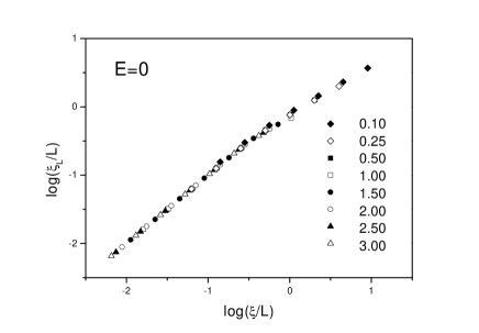
Figure 1: Scaling function (for the second moment) for the 2-D Anderson model. $\xi=\xi(\sigma)=\xi_{\infty}$ is the scaling parameter necessary to scale numerical data onto the same curve. Values of the disorder $\sigma$ are indicated.

One notices that the idea of numerical scaling has a weak point; one starts from the assumption that self-averaging quantities exist. The analytic solution presented in the present paper, section 3, offers in principle the possibility to clarify the problems connected with the numerical scaling procedure. The analytic equations treat from the very start a system in the thermodynamic limit ($L=\infty$), because the integer $m\in(-\infty,+\infty)$ in eq.(29). A transition to a finite system ($L<\infty$) in this context is rather trivial and corresponds simply to the transition from the Fourier integral, eq.(44) to the Fourier series. Thus we arrive from the filter-function in the form of eq.(64) at another equation:

$$H^{-1}(z)=1-\frac{\sigma^{2}}{L}\frac{(z+1)}{(z-1)}\sum_{j=0}^{L-1}\frac{1}{w^{2}-{\mathcal{E}}^{2}(k_{j})},$$ (77)

$$k_{j}=\frac{2\pi j}{L}.$$ (78)

The difference is large. The filter (64) has a multiplicity of solutions: the unit circle $|z|=1$ divides the complex plane into two analytic domains. For a finite system one has only one solution, the unit circle $|z|=1$ does not play a role anymore. The filter (77) corresponds to only one phase, where all states are localized. Mathematically this means that between the possible poles $z=\lambda_{i}$ of the function (77) there always exist the pole $\lambda_{max}>1$, and the filter is unstable. If one defines the localization length as $\xi_{L}=1/\gamma_{L}$, where according to the definition by using the second moments $\lambda_{max}=\exp(2\gamma_{L})$, then this length is always finite.

The physical reason for this result is rather clear: in the $n$-direction the system remains infinite since the $Z$-transform always “feels” the true asymptotic behavior. Fixing a finite size $L$ in the $m$-direction effectively renders the system a one-dimensional one at large scales, hence the corresponding behaviour (full localization). From this point of view, $\xi_{L}$ is essentially the crossover length form 2-D to 1-D behavior.

Let us do now a typical scaling study for the localization length $\xi_{L}$ at the band centre, $E=0$. We have found that the scaling parameter $\xi_{\infty}$ is identical with the value $\xi$, where $\xi=1/\gamma$ and $\gamma$ is defined in eq.(70). Disregarding for the moment the fact that one commonly uses a different definition of the localization length $\xi_{L}$ via the log-definition, we arrive qualitatively at the same results as numerical scaling[3]. There exists a scaling function, Fig.1, which is typical for 2-D systems and whose behaviour one commonly interprets as complete localization in 2-D dimensions. The corresponding scaling parameter is, however, identical with the localization length $\xi$ in the insulating phase. I.e. numerical scaling is not capable to analyze a system consisting of two phases. This approach to the problem with particular solutions of different asymptotic behaviour, $\gamma\equiv 0$ or $\gamma\neq 0$, always sees only one diverging solution ($\gamma\neq 0$).

5 Conclusion

The basic idea of the present work is to apply signal theory to the Anderson localization problem. We interpret certain moments of the wave function as signals. There is then in signal theory a qualitative difference between localized and extended states: The first ones correspond to unbounded signals and the latter ones to bounded signals. In the case of a metal-insulator transition extended states (bounded signals) transform into localized states (unbounded signals). Signal theory shows that it is possible in this case to find a function (the system function or filter), which is responsible for this transformation. The existence of this transformation in a certain region of disorder and energy simply means that the filter looses its stability in this region. The meaning of an unstable filter is defined by a specific pole diagram in the complex plane. These poles also define a quantitative measure of localization. Thus it is possible here to determine the socalled generalized Lyapunov exponents as a function of disorder and energy.

For pedagogical reasons we have analyzed in this paper first the 1-D case. Here no new results are obtained. All states are localized for arbitrary disorder. The aim of this section consists in showing to the uninitiated reader a possible alternative to the traditional mathematical tools of dealing with Anderson localization and to interpret its content. The power of the approach comes only to its full bearing when it proves possible to find analytically the filter function also for the 2-D case. Although the filter is quite in general defined by an integral, it is possible to give a representation in terms of radicals. As a consequence we have been able to find an exact analytical solution for the generalized Lyapunov exponents for the well-known and notorious Anderson problem in 2-D. In this way the phase diagram is obtained.

The approach suggested in the present paper does not in any way represent the complete solution to the problem of Anderson localization in 2-D. The very important topic of the transport properties of disordered systems lies outside the presumed region of applicability of the method. The results of the studies give us a few answers to existing questions but open up even more questions. We have only considered the phase diagram of the system. The theory permits us to ascertain to which class of problems Anderson localization belongs.

In the 1-D case all states are localized for infinitesimally small disorder in complete agreement with the theoretical treatment of Molinari [14]. In the 2-D case we have shown that in principle there is the possibility that the phase of delocalized states exists for a non-interacting electron system. This phase has its proper existence region and it belongs to the marginal type of stability. All states with energies $|E|>2$ are localized at arbitrarily weak disorder. For energies and disorder, where extended states may exist we find a coexistence of these localized and extended states. Thus the Anderson transition should be regarded as a first order phase transition. The argument of Mott that extended and localized states cannot be found at the same energy is probably not applicable in our case as the solutions for the two relevant filter functions do not mix. This has to be worked out in detail in the future. Also the role of different disorder realizations has to be elaborated, which could be a source of the observed phenomena.

Our findings can in principle explain the experimental results of Kravchenko et al. [10] on films of a-Si. They are also in agreement with the experimental findings of Ilani et al [12, 13] which showed the coexistence of phases. Although one has to be cautious in concluding from our results directly onto specific experimental situations our theory is the first one to be in accord with experiment for 2-D systems.

We hope that the presented results contribute to the solution of the existing contradictions between theory and experiment, and also between different experimental results.

The qualitative diagnosis which we propose here is in several aspects different from the predictions of prevailing theories, scaling theory, mean field and perturbation theory. It has to be stated here that much work still remains to be done both via the present approach as via other established approaches.

1. The Anderson problem belongs to the class of critical phenomena. It is known from the scientific literature that in such a case one encounters in general a poor convergence behaviour of approximations [20, 21], which in their basis contain a mean field approach. To cite an example: the exact solution of Onsager for the 2-D Ising model is in complete disagreement with the Landau theory of phase transitions (mean field theory) [20]. All critical exponents differ in the two approaches. Yet there is at least a qualitative agreement between the two theories: the Landau theory describes second order phase transitions and the exact Onsager theory confirms this aspect.

2. For the Anderson problem the outlook on the theories might also be far reaching, if our approach should prove to be correct. All presently accepted theories derive here from the scaling idea which is in turn based on the assumption that the Anderson transition belongs to the class of second order phase transitions. This basic idea is up to now a hypothesis which cannot be proved in the absence of the exact solution. One has assumed that averaged or self-averaging quantities are always physical quantities. And every theory had the direct aim to calculate such quantities. Our exact solution for the phase diagram, however, indicates that in this system the coexistence of phases is possible, i.e. that the Anderson transition should be regarded as a phase transition of first order.

3. For a phase transition of first order with a coexistence of phases there surely also exist self-averaging quantities, whose fluctuations are small. The quantities, however, tend to be unphysical because the average over an ensemble includes an average over the phases. Physically meaningful in this case are only the properties of the pure phases. Consequently one requires a new idea to calculate the transport properties of the disordered systems. We can at the present time only surmise that this future theory of transport properties will calculate the transport properties with the help of equations which have the property of a multiplicity of solutions. This theory should also formulate in a new way the average over the ensemble of random potentials in order to arrive at the properties of the pure phases.

References

- [1] P.W. Anderson, Phys. Rev. 109, 1492 (1958).
- [2] P.A. Lee and T.V. Ramakrishnan, Rev. Mod. Phys. 57, 287 (1985).
- [3] B. Kramer and A. MacKinnon, Rep. Prog. Phys. 56, 1469 (1993).
- [4] M. Janssen, Phys. Rep. 295, 2 (1998).
- [5] N.F. Mott and W.D. Twose, Adv. Phys. 10, 107 (1961).
- [6] E. Abrahams, P.W. Anderson, D.C. Licciardello, and T.V. Ramakrishnan, Phys. Rev. Lett. 42, 673 (1979).
- [7] P.W. Anderson, D.J. Thouless, E. Abrahams, and D.S. Fisher, Phys. Rev. B 22, 3519 (1980).
- [8] I.Kh. Zharekeshev, M. Batsch, and B. Kramer, Europhys. Lett. 34, 587 (1996).
- [9] J.W. Kantelhardt and A. Bunde, Phys. Rev. B, 66, 035118 (2002).
- [10] S.V. Kravchenko, D. Simonian, M.P. Sarachik, W. Mason, and J.E. Furneaux, Phys. Rev. Lett. 77, 4938 (1996).
- [11] E. Abrahams, S.V. Kravchenko, M.P. Sarachik, Rev. Mod. Phys. 73, 251 (2001).
- [12] S. Ilani, A. Yacoby, D. Mahalu and Hadas Shtrikman. Science 292, 1354 (2001)
- [13] S. Ilani, A. Yacoby, D. Mahalu and H. Shtrikman, Phys. Rev. Lett. 84, 3133 (2000)
- [14] L. Molinari. J.Phys.A: Math. Gen. 25, 513 (1992).
- [15] T.F. Weiss. Signals and systems. Lecture notes. http:// umech.mit.edu/ weiss/ lectures.html; K.L. Kosbar. Digital signal processing. http:// www.siglab.ee.umr.edu/ ee341/ index.html
- [16] K. Ishii, Suppl. Prog. Theor. Phys. 53, 77 (1973).
- [17] M. Kappus and F. Wegner, Z. Phys. B Condensed Matter 45, 15 (1981).
- [18] J. B. Pendry and E. Castano, J. Phys. C: Solit State Phys. 21, 4333 (1988).
- [19] D.J. Thouless, in: Ill-condensed Matter, Eds. R. Balian, R. Maynard, G. Toulouse, Amsterdam, New York: Nort-Holland,1979, p.1.
- [20] H.E. Stanley, Introduction to Phase Transition and Critical Phenomena (Oxford Univ. Press, New York, 1971).
- [21] R.J.Baxter, Exactly Solved Models in Statistical Mechanics (Academic Press, London, New York, 1982).
- [22] R.Balescu. Equilibrium and Non-equilibrium Statistic Mechanics (Wiley, New York, 1975).