What do phase space methods tell us about
disordered quantum systems?
Gert-Ludwig Ingold, André Wobst, Christian Aulbach,
and Peter Hänggi
Institut für Physik, Universität Augsburg, D-86135 Augsburg
to be published in

“The Anderson Transition and its Ramifications – Localisation, Quantum Interference, and Interactions”,

Lecture Notes in Physics, http://link.springer.de/series/lnpp/

© Springer Verlag, Berlin-Heidelberg-New York

What do phase space methods tell us about disordered quantum systems?

1 Introduction

At a summer school held in fall 1991 at the PTB in Braunschweig, Bernhard Kramer proposed a book project that should encompass novel solid state research topics ranging from quantum transport to quantum chaos. This very book finally appeared at the end of 1997 under the title “Quantum transport and dissipation” ingold:qtad98 . Compiled between the book covers is a series of topics, some of which are usually not connected with each other in present day’s research. The main subject in the first chapter is coherent transport in disordered systems. The last chapter, on the other hand, dwells on concepts such as phase space, Wigner and Husimi functions, and alike. In any case, in the description of disordered systems we do not find many works that explicitly make use of phase space concepts. This is so, although the existence of a mapping between the Anderson model and the kicked rotor ingold:fishm82 indeed suggests that methods employed in quantum chaos may advantageously be used to elucidate the physics at work in disordered quantum systems.

There exists, however, another, almost obvious physical motivation to utilize the powerful phase space concepts to study disordered quantum systems: as a function of the disorder strength, the nature of the eigenstates changes from ballistic to localized behavior, containing possibly in-between a diffusive regime ingold:krame93 . In the case of ballistic transport it is appropriate to think in terms of plane waves which are occasionally scattered by the weak disorder potential. Then a momentum space description clearly imposes itself. For strong disorder, however, the natural physical space is real space. A unified description, being valid at arbitrary disorder strength, can thus be achieved by focusing on suitable (quantum) phase space concepts.

2 Phase space methods in quantum mechanics

When an attempt is made to represent a quantum state in phase space, there are two observations which deserve our attention. First, phase space combines conjugate quantum observables which brings into play a Heisenberg uncertainty relation. While in classical mechanics, the state of a point particle can be described in phase space with infinite precision, this no longer holds true in quantum mechanics. Therefore, we expect some difficulties if for quantum systems one attempts to obtain perfect resolution in phase space. Second, the full information about a quantum state is contained already in the corresponding wave function which can either be expressed in position or momentum space representation. Thus, the phase space representation of a quantum state cannot provide more information than the wave function itself. This information, however, may be presented in a more advantageous form, as we shall demonstrate next.

2.1 The Wigner function

As a first possibility to define a phase space representation of a quantum state possessing the wave function $\psi(x)$ we introduce the Wigner function

$$W(x,k)=\int\mathrm{d}y\mathrm{e}^{{\rm i}ky}\psi^{*}(x+\frac{y}{2})\psi(x-\frac{y}{2})\,.$$ (1)

Here, and in the following we use the wave number $k$ instead of the momentum $p=\hbar k$. The definition (1) is useful and appropriate as can be seen by considering the moments of position and momentum observables. Upon evaluation of the momentum integral, one readily finds that

$$\int\frac{\mathrm{d}x\mathrm{d}k}{2\pi}x^{n}W(x,k)=\int\!\mathrm{d}x\,x^{n}|\psi(x)|^{2}.$$ (2)

With a little more effort one further can establish that

$$\int\frac{\mathrm{d}x\mathrm{d}k}{2\pi}k^{n}W(x,k) =\int\!\!\mathrm{d}x\int\!\!\mathrm{d}y\int\frac{\mathrm{d}k}{2\pi}\left[(-{\rm i})^{n}\frac{\mathrm{d}^{n}}{\mathrm{d}y^{n}}\mathrm{e}^{{\rm i}ky}\right]\psi^{*}(x)\psi(x-y)$$ (3)

$$=\int\!\!\mathrm{d}x\,\psi^{*}(x)\left(\frac{1}{{\rm i}}\frac{\mathrm{d}}{\mathrm{d}x}\right)^{n}\psi(x)\,.$$

A generalization to moments containing both position and momentum operators is possible if a Weyl ordering for the operators is respected (for further details see ingold:hille84 ).

To start, it is instructive to consider a few special quantum states of simple structure which also play a key role in the discussion of disordered systems. Let us begin with a plane wave, i.e. $\psi(x)=\exp({\rm i}k_{0}x)/\sqrt{2\pi}$. Inserting this wave function into (1) one finds

$$W(x,k)=\int\frac{\mathrm{d}y}{2\pi}\mathrm{e}^{{\rm i}(k-k_{0})y}=\delta(k-k_{0})\,.$$ (4)

The intermediate result emphasizes the fact that the off-diagonal contributions in (1), which are parameterized by the coordinate $y$, contain the information about the momentum. For a localized state, $\psi(x)=\delta(x-x_{0})$, the Wigner function emerges as

$$W(x,k)=\mathrm{e}^{2{\rm i}k(x-x_{0})}\delta(x-x_{0})=\delta(x-x_{0})\,.$$ (5)

Next we consider a quantum state localized at two positions, i.e. $\psi(x)=[\delta(x+a)+\delta(x-a)]/\sqrt{2}$. Proceeding as before, one obtains the Wigner function

$$W(x,k)=\frac{1}{2}\left[\delta(x+a)+\delta(x-a)\right]+\cos(2ka)\delta(x)\,.$$ (6)

The first two terms describe the localization of the particle at $x=\pm a$. In addition, there occurs an oscillatory term in the middle between the two localization centers which accounts for the coherent superposition of two localized states. This simple example demonstrates that the Wigner function generally is not positive even though it could be treated as a phase space density in (2) and (3). This characteristic feature is a direct consequence of the fact that by virtue of the definition (1) one attempts to define a phase space representation which allows for perfect localization in position and momentum as indicated by the results (4) and (5). This formal attempt to circumvent the Heisenberg uncertainty relation is generally paid for by negative parts of the Wigner function.

Thus far, we have considered a particle on a continuous and infinitely extended one-dimensional state space. The situation changes when we try to apply phase space concepts to the Anderson model of disordered systems. For such a lattice model the integral in (1) has to be replaced by a sum. Moreover, in numerical calculations, the system size has to be taken finite. This results in a phase space that is twisted to a torus so that additionally periodic boundary conditions appear in momentum space apart from those usually imposed in real space. Therefore, interference terms in momentum space analogous to those appearing in real space as in (6) occur also across the boundaries of the Brillouin zone. Such artifacts can also be understood as arising from the discretization of the integral in (1) due to the lattice structure of the model. In particular for the states located at the boundaries of the Brillouin zone, the wave number $k$ is so large that a discretized version of the Fourier integral no longer represents a good approximation. The usage of Wigner functions for lattice models therefore becomes problematic.

In Fig. 1 we present an example for the Wigner function of an eigenstate of the Anderson model at relatively low disorder. While a certain spatial localization has already set in, two dominant wave numbers $\pm k$ can still be clearly recognized. At $k=0$, interference effects analogous to those found in (6) are visible while the two low ridges at larger wave numbers represent the artifacts due to the lattice structure of the Anderson model discussed in the previous paragraph.

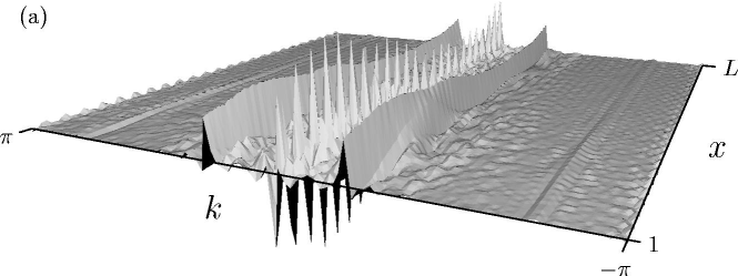
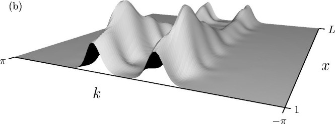
Figure 1: (a) Wigner function and (b) Husimi function for an eigenstate of the Anderson model

2.2 The Husimi function

The above discussed shortcomings of the Wigner function can be circumvented by use of the so-called Husimi function. The latter one is obtained from the Wigner function by a Gaussian smearing according to

$$\rho(x,k)=\frac{1}{\pi}\int\!\!\mathrm{d}x^{\prime}\mathrm{d}k^{\prime}\exp\left[-\frac{(x-x^{\prime})^{2}}{2\sigma^{2}}-2\sigma^{2}(k-k^{\prime})^{2}\right]W(x^{\prime},k^{\prime})\,.$$ (7)

Even though one might assume that one discards information by transforming the Wigner function $W(x,k)$ into the Husimi function $\rho(x,k)$, this is actually not the case as one can show by inverting (7): The Wigner function can then be recast as

$$W(x,k) =$$ (8)

$$\int\frac{\mathrm{d}u\mathrm{d}v}{2\pi}\frac{\mathrm{d}x^{\prime}\mathrm{d}k^{\prime}}{2\pi}\exp\left[\frac{\sigma^{2}u^{2}}{2}+\frac{v^{2}}{8\sigma^{2}}+{\rm i}(x^{\prime}-x)u+{\rm i}(k^{\prime}-k)v\right]\rho(x^{\prime},k^{\prime})\,.$$

The existence of the integrals is guaranteed by the inherent asymptotic decay of the Husimi function provided that the integrals over $x^{\prime}$ and $k^{\prime}$ are evaluated first.

From a physical point of view, the most important aspect of the Gaussian smearing introduced in (7) is that the Heisenberg uncertainty relation is now accounted for in a natural way. The Husimi function will never localize a quantum state in phase space beyond the limits set by the requirement $\Delta x\Delta k\geq 1/2$. In return, the Husimi function yields a nonnegative-valued phase space distribution. Indeed, by inserting (1) into (7) one can express the Husimi function in terms of the wave function $\psi(x)$ as the squared quantity

$$\rho(x,k)=\left|\int\mathrm{d}x^{\prime}\psi(x^{\prime})\frac{1}{(2\pi\sigma^{2})^{1/4}}\exp\left[-\frac{(x^{\prime}-x)^{2}}{4\sigma^{2}}-{\rm i}kx^{\prime}\right]\right|^{2}\,,$$ (9)

which manifestly is nonnegative. According to (9), the Husimi function may be viewed as the projection of the wave function onto a minimal uncertainty state or, using the language of quantum optics, onto a coherent state. At this point, the width $\sigma$ is still a parameter which can be chosen freely. We will fix its value later on when applying these phase space concepts to the Anderson model.

Yet another aspect of the Gaussian smearing pertains to the artifacts mentioned in the previous section for the Wigner function on a lattice. While in (1) all values of $y$ contribute, this is no longer the case for the Husimi function where the convolution with a Gaussian restricts the difference in the arguments of the two wave functions. In fact, even the interference term appearing in the Wigner function (6) for a continuum model is strongly suppressed in the corresponding Husimi function provided the distance $a$ is sufficiently larger than the width $\sigma$; this is evident from

$$\rho(x,k) =\frac{1}{2\sqrt{2\pi\sigma^{2}}}\bigg{[}\exp\left(-\frac{(x-a)^{2}}{2\sigma^{2}}\right)+\exp\left(-\frac{(x+a)^{2}}{2\sigma^{2}}\right)$$ (10)

$$\hskip 130.08731pt+2\exp\left(-\frac{x^{2}}{2\sigma^{2}}-\frac{a^{2}}{2\sigma^{2}}\right)\cos(2ka)\bigg{]}\,.$$

A comparison of the Wigner function in Fig. 1 and the Husimi function in Fig. 1 demonstrates the effect of the Gaussian smearing. The spatial localization and the two mainly contributing wave numbers are the dominant features of the Husimi function. The interferences leading to negative contributions to the Wigner function have almost disappeared except for some wiggles which, however, do not render the Husimi function negative. Finally, the features stemming from the lattice have now disappeared.

2.3 Inverse participation ratio

The Husimi function, in particular for quantum states at intermediate disorder strengths, does contain a rich structure. In general, it is desirable for various reasons to reduce this wealth of information and to characterize the state by a single number which is derived from the Husimi function. First, in clear contrast to the one-dimensional case depicted in Fig. 1 it is generally not possible to visualize the Husimi function for systems in two and higher space dimensions. Second, the details of the Husimi functions depend sensitively on the chosen disorder realization. In order to perform averages, it is necessary to reduce the characterization of the states to a number.

Since the Husimi function is nonnegative, in principle all quantities familiar from classical phase space analysis can be employed in the quantum case as well. One possibility is given by the so-called Wehrl entropy ingold:wehrl79

$$S=-\int\frac{\mathrm{d}x\mathrm{d}k}{2\pi}\rho(x,k)\ln[\rho(x,k)]\,,$$ (11)

which has been used, e.g., in the discussion of the driven rotor ingold:gorin97 . The above-mentioned existence of a mapping between the kicked rotor and the Anderson model has motivated a study of the latter by means of the Wehrl entropy ingold:weinm99 .

From a numerical point of view, it is advantageous to linearize the Wehrl entropy (11). Replacing $\ln(x)$ by its linear approximation $x-1$, one obtains $-x\ln(x)\approx x-x^{2}$. The approximation shows qualitatively the some behavior as the original function and, in particular, yields the same values at the boundaries at $x=0$ and $1$. Performing this linearization in (11), the first order term gives rise to a constant due to normalization and we are left with the second order term, the inverse participation ratio (IPR) in phase space

$$P=\int\frac{\mathrm{d}x\mathrm{d}k}{2\pi}[\rho(x,k)]^{2}\,.$$ (12)

While both the Wehrl entropy $S$ and the phase space IPR $P$ are entirely determined in terms of the wave function $\psi(x)$, it is necessary for the evaluation of the Wehrl entropy to first calculate the Husimi function explicitly. This requires a significant numerical effort which can be reduced by resorting to the phase space IPR ingold:manfr00 . In turn, this makes possible the study of the Anderson model in two and even in three dimensions ingold:wobst02 . Inserting (9) into (12) one obtains the phase space IPR expressed directly in terms of the wave function as

$$P=\frac{1}{8\sqrt{\pi}\sigma}\int\!\mathrm{d}u\left|\int\!\mathrm{d}v\,\psi\left(\frac{u-v}{2}\right)\psi\left(\frac{u+v}{2}\right)\exp\left(-\frac{v^{2}}{8\sigma^{2}}\right)\right|^{2}\,.$$ (13)

Apart from the numerical aspects, another advantage relates to the fact that inverse participation ratios may be defined as well in real and momentum space, i.e.,

$$P_{x}=\int\!\mathrm{d}x\,|\psi(x)|^{4}\qquad\mathrm{and}\qquad P_{k}=\int\!\mathrm{d}k\,|\widetilde{\psi}(k)|^{4}\,,$$ (14)

where $\widetilde{\psi}(k)$ is the wave function in momentum representation. The availability of the inverse participation ratio in different spaces allows for instructive physical comparisons. The real space IPR $P_{x}$ is a well studied quantity as it is related to the return probability of a diffusing particle ingold:thoul74 while the phase space IPR has recently been used to describe the complexity of quantum states ingold:sugit02 ; ingold:sugit01 . We add that a quantity containing information similar to the phase space IPR can be defined on the basis of marginal distributions in real and momentum space ingold:varga02 .

In order to demonstrate that it is justified to refer to the above-mentioned quantities as inverse participation ratios, we consider a few special cases for quantum states on a one-dimensional lattice with $L$ lattice sites. Let us first assume that the state is localized on a single site. Then we find $P_{x}=1$ and $P_{k}=1/L$. The inverse of these results indeed indicates that in real space the state occupies only one site while in momentum space $L$ sites are occupied. In phase space, one obtains $P=1/2\sqrt{\pi}\sigma$ which primarily reflects the Gaussian width in real space.

As a second example, we consider a real-valued ballistic wave function at momentum $\bar{k}$, i.e. $\psi(x)=\sqrt{2/L}\cos(\bar{k}x)$. In real and momentum space, the inverse participation ratios become $P_{x}=3/2L$ and $P_{k}=1/2$, respectively. The first result accounts for the nonuniform extension in real space while the latter indicates the contribution of the two momenta $\pm\bar{k}$. For $\bar{k}\neq 0,\pm\pi$, the phase space IPR $P=(\sigma\sqrt{\pi}/L)[1+2\exp(-4\sigma^{2}\bar{k}^{2})]$ depends on the distance between the two contributing momenta.

So far, we have not specified the width $\sigma$ entering both, the definition (9) of the Husimi function and the results for the phase space IPR $P$ mentioned in the previous two paragraphs. Although one is rather free in choosing $\sigma$, the most impartial choice consists in selecting an equal relative resolution in real and momentum space, i.e. $\Delta x/L=\Delta k/2\pi$. Together with the requirement of minimal uncertainty, $\Delta x\Delta k=1/2$, one finds $\Delta x=\sigma=\sqrt{L/4\pi}$. For our two examples mentioned above (which will appear later in the limits of vanishing and very strong disorder) this implies, that the IPR $P$ will scale like $1/\sqrt{L}$ as a function of system size. This result for one-dimensional systems is found to generalize to $P\sim L^{-d/2}$ in $d$ dimensions.

An intuition for the differences between inverse participation ratios in real and momentum space, on the one hand, and the IPR in phase space, on the other hand, can be obtained by considering the resolution provided by the wave function and the Husimi function in real and momentum space. The vertical gray stripe on the left in Fig. 2 corresponds to the real space wave function. Independent of system size, this wave function always leads to perfect resolution in real space. The price to be paid, however, consists in the absence of any resolution in momentum space. The converse holds true for the momentum space wave function. The situation is quite different for the Husimi function symbolized by the gray disk in Fig. 2. Although the discussion can be generalized ingold:ingol02 , we will consider the case where $\sigma\sim\sqrt{L}$. Then, structures occurring on $\sqrt{L}$ lattice points, or less, cannot be resolved. While this resolution becomes worse as the system size is increased, the resolution relative to the system size improves with $1/\sqrt{L}$. For large system sizes, the phase space approach therefore allows for a detailed description of a quantum state both in real and momentum space, while a specific wave function representation will always neglect one of the two possibilities.

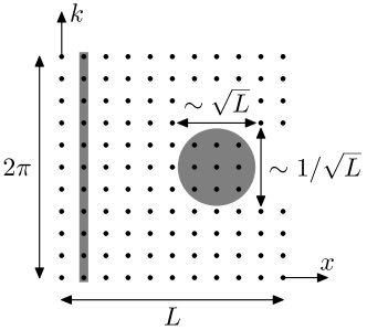
Figure 2: The different phase space resolution provided by real space wave function and Husimi function is visualized by the gray shaded areas on the left and right, respectively

3 Anderson model in phase space

In the preceding section we have demonstrated that a phase space approach indeed presents advantages when both, real and momentum space properties are of interest as it is the case for disordered systems when the disorder strength is varied from zero to infinity. Although, in principle, the Husimi function is equivalent to the wave function, it will make the relevant information more readily accessible. We next want to illustrate this very fact by considering the Anderson model for disordered systems. Its Hamiltonian ingold:ander58

$$H=-t\sum_{<\mathbf{x},\mathbf{x^{\prime}}>}(|\mathbf{x^{\prime}}\rangle\langle\mathbf{x}|+|\mathbf{x}\rangle\langle\mathbf{x^{\prime}}|)+W\sum_{n}v_{n}|\mathbf{x}\rangle\langle\mathbf{x}|$$ (15)

is defined on a $d$ dimensional square lattice with $L$ sites in each direction. In order to avoid boundary effects, periodic boundary conditions are imposed. The first term describes the kinetic energy which allows for hopping between nearest neighbor sites $<\mathbf{x},\mathbf{x^{\prime}}>$. In the following, the hopping matrix element will set the energy scale, i.e. $t=1$. The second term on the right-hand side of (15) represents the disordered on-site potential where the energies $v_{n}$ are independently drawn from a box distribution on the interval $[-1/2;1/2]$. The respective disorder strength is then determined by $W$.

3.1 Husimi functions

Before we investigate the inverse participation ratio for the Anderson model, it is instructive to first take a look at the underlying Husimi functions. Since a visualization is readily possible only for one-dimensional models, we compare in Fig. 3 the one-dimensional Anderson model and the Aubry-André model ingold:aubry80 . The latter is based on a periodic potential $\lambda\sum_{n}\cos(2\pi\beta n)|n\rangle\langle n|$ replacing the disorder potential in (15). Choosing $\beta$ as the golden mean, $(\sqrt{5}-1)/2$, the potential is incommensurate with the underlying lattice and displays a phase transition from delocalized to localized states ingold:aubry80 . We have chosen this model for comparison since its phase space IPR is comparable to that obtained for the two- and three-dimensional Anderson model ingold:ingol02 . In Fig. 3, the Aubry-André model therefore serves as a substitute for the higher-dimensional Anderson models.

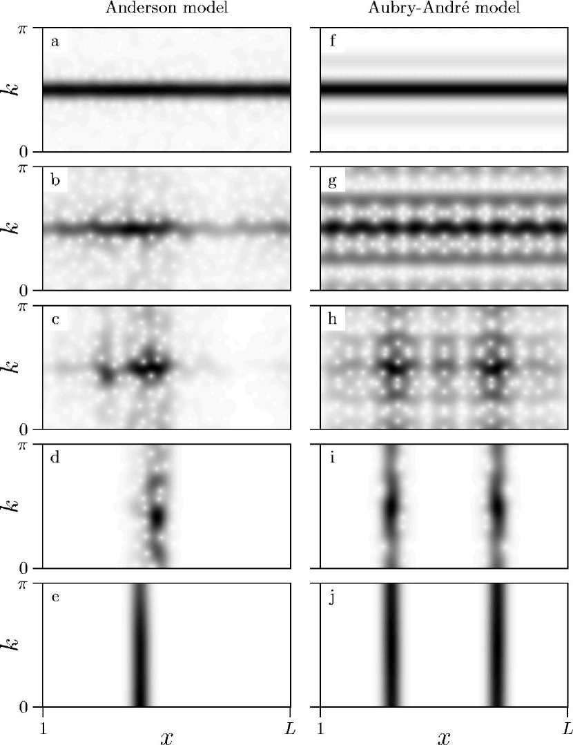
Figure 3: Husimi functions for (a–e) the Anderson model with disorder strength $W=0.1,1,2,4$, and $40$ and (f–j) the Aubry-André model with potential strength $\lambda=0.1,1.5,2,2.5$, and $10$ for a state close to the band center and a system size $L=377$. In view of the symmetry $\rho(x,-k)=\rho(x,k)$ only the upper half of the phase space is shown

Before we discuss in further detail the Husimi functions depicted in Fig. 3, we mention that for real wave functions the Husimi function, according to its definition (9), respects the symmetry $\rho(x,k)=\rho(x,-k)$. It is therefore sufficient to plot the Husimi functions solely for positive momenta from which the lower part may be reconstructed as a mirror image with respect to $k=0$.

The Husimi functions for the limiting cases of very weak and very strong potential depicted in Figs. 3(a) and 3(e) for the Anderson model and Figs. 3(f) and 3(j) for the Aubry-André model can readily be interpreted in terms of states localized either in momentum or in real space. In addition, in Fig. 3(f) the coupling between plane waves due to the periodic potential becomes visible while the localization at two sites seen in Fig. 3(j) arises because the calculation was restricted to the class of antisymmetric states ingold:thoul83 . Furthermore, we keep the state number fixed while passing through avoided crossings so that states may be localized at different positions as a function of potential strength (cf. e.g. Figs. 3(d) and 3(e)).

More interesting than the interpretation of the Husimi function in the limiting cases is a discussion of the transition from plane waves for a weak potential to spatially localized states for a strong potential. The one-dimensional Anderson model and the Aubry-André model display two different scenarios with the latter being also characteristic for higher-dimensional Anderson models (cf. Sect. 3.2).

For the one-dimensional Anderson model, the Husimi function for a plane wave (Fig. 3(a)) contracts in real space (Fig. 3(b)) and displays a very well localized core at intermediate disorder strength $W$ (Fig. 3(c)). A further increase of the potential strength leads to a spreading in momentum direction (Fig. 3(d)) and finally a state localized in real space (Fig. 3(e)) is approached.

For the Aubry-André model the scenario is quite different. As mentioned above, already a weak potential strength $\lambda$ can lead to a coupling between plane waves of very different momenta (Fig. 3(f)). This type of coupling is accompanied by an increased filling of phase space (Fig. 3(g)) up to potential strengths $\lambda$ located just below the critical value of $\lambda=2$ where the localization transition takes place (Fig. 3(h)). There, for increasing system size, a more and more abrupt contraction in phase space occurs, cf. Fig. 3(i). Finally, for very strong potentials, the Husimi function of a localized antisymmetric state depicted in Fig. 3(j) forms.

3.2 Inverse participation ratios

While the Husimi functions depicted in Fig. 3 nicely elucidate the phase space behavior of a state as a function of potential strength, a more quantitative analysis is desirable. On the basis of inverse participation ratios, a study of the higher-dimensional Anderson model becomes feasible and averages over disorder realizations can be performed. This in turn will allow us to draw general conclusions about the physics that rules the localization transition in the Anderson model.

In Fig. 4 we present distributions of the inverse participation ratios $P_{x}$, $P$, and $P_{k}$ in real space, phase space, and momentum space, respectively, for the Anderson model in one, two, and three dimensions. The distributions have been obtained by diagonalizing the Anderson model for 50 disorder realizations in $d=1$ and $2$ and taking half of the eigenstates around the bandcenter for each realization. In $d=3$ it was sufficient to consider only 20 disorder realizations.

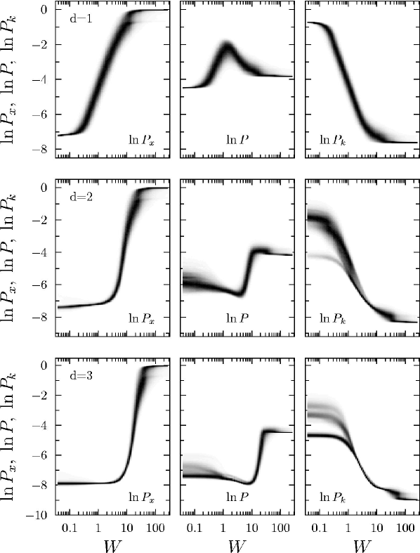
Figure 4: Distribution of inverse participation ratios in real space (left), phase space (middle), and momentum space (right) for the Anderson model in $d=1$ (upper row, $L=2048$), $d=2$ (middle row, $L=64$), and $d=3$ (lower row, $L=20$)

Upon comparing the real space IPRs for the three different dimensions, no qualitative differences can be seen. The overall behavior shows an increase of $P_{x}$ (left column) with increasing potential strength reflecting the spatial localization of the wave functions. Correspondingly, the momentum space IPR (right column) decreases with increasing potential strength.

In clear contrast, the phase space IPR behaves qualitatively different for the Anderson model in $d=1$ and $d\geq 2$. For $d=1$, the peak in $P$ is consistent with our observations for the Husimi function in Figs. 3(a–e), namely the contraction of the Husimi function at intermediate disorder strength.

For $d=2$ and $3$, the behavior of the phase space IPR rather corresponds to what we have observed for the Husimi function of the Aubry-André model in Figs. 3(f–j). With increasing potential strength, the Husimi function spreads in phase space implying a decrease of $P$. Then, at the transition, a sudden contraction occurs, implying a jump to relatively large values of $P$. This scenario can be understood in physical terms as follows. The large spread in phase space is associated with the presence of a diffusive regime which is known to exist in $d=2$ and larger. This interpretation is corroborated by a comparison with results from energy level statistics ingold:wobst02 . The jump in $P$, on the other hand, indicates the Anderson transition ingold:abrah79 ; ingold:lee85 . Here, one might object that the case $d=2$ is the marginal case where strictly speaking no phase transition occurs. One finds indeed, that both, the minimum and the maximum of $P$, shift towards vanishing disorder as the system size is increased ingold:wobstxx . In contrast, in $d=3$, the minimum of $P$ shifts to larger disorder strength $W$, while the maximum shifts in the opposite direction, in agreement with the existence of the Anderson transition.

A comparison of the Husimi functions for the one-dimensional Anderson model and the Aubry-André model reveals the differences between the Anderson model in $d=1$ and in higher dimensions. In the one-dimensional Anderson model, a weak disorder potential predominantly couples a plane wave to other, energetically almost degenerate plane waves. Therefore, the coupling occurs between plane waves of almost the same momentum. Due to the finite resolution in phase space, this coupling cannot be observed in momentum space. In real space, however, the coupling results in large scale variations of the Husimi function which in the end cause a contraction in phase space as discussed above. In clear contrast, for the Aubry-André model the situation is quite different: Here, the coupling predominantly occurs to distant momentum values as can be seen in Fig. 3(f). This finally leads to a spreading of the Husimi function in phase space ingold:ingol02 . The very same scenario is valid for the Anderson model in two and higher dimensions. Again, there exist energetically almost degenerate momenta which are very different from those present in the original plane wave. The coupling due to a weak disorder potential thus again leads to a spreading in phase space. On the other hand, perturbation theory for strong disorder shows that the limiting value of the phase space IPR for large $W$ is approached from above ingold:wobstxx . Therefore, a jump from small to large values of $P$ arises and thus a phase transition (in $d=3$) is to be expected at an intermediate disorder strength $W$.

In conclusion, these considerations in phase space in terms of concepts such as the Husimi function and the corresponding inverse participation ratio prove indeed very valuable in order to explore in greater detail the physics for a class of quantum systems which is so dear to Bernhard Kramer, namely disordered quantum systems ingold:krame93 .

References

- (1) T. Dittrich, P. Hänggi, G.-L. Ingold, B. Kramer, G. Schön, W. Zwerger: Quantum transport and dissipation (Wiley-VCH 1998)
- (2) S. Fishman, D. R. Grempel, R. E. Prange: Phys. Rev. Lett. 49, 509 (1982)
- (3) B. Kramer, A. MacKinnon: Rep. Prog. Phys. 56, 1469 (1993)
- (4) M. Hillery, R. F. O’Connell, M. O. Scully, E. P. Wigner: Phys. Rep. 106, 121 (1984)
- (5) A. Wehrl: Rep. Math. Phys. 16, 353 (1979)
- (6) T. Gorin, H. J. Korsch, B. Mirbach: Chem. Phys. 217, 145 (1997)
- (7) D. Weinmann, S. Kohler, G.-L. Ingold, P. Hänggi: Ann. Phys. (Leipzig), 8, SI-277 (1999)
- (8) G. Manfredi, M. R. Feix: Phys. Rev. E 62, 4665 (2000)
- (9) A. Wobst, G.-L. Ingold, P. Hänggi, D. Weinmann: Eur. Phys. J. B 27, 11 (2002)
- (10) D. J. Thouless: Phys. Rep. 13, 93 (1974)
- (11) A. Sugita, H. Aiba: Phys. Rev. E 65, 036205 (2002)
- (12) A. Sugita: arXiv:nlin.CD/0112042
- (13) I. Varga, J. Pipek: arXiv:cond-mat/0204041
- (14) G.-L. Ingold, A. Wobst, Ch. Aulbach, P. Hänggi: Eur. Phys. J. B 30, 175 (2002)
- (15) P. W. Anderson: Phys. Rev. 109, 1492 (1958)
- (16) S. Aubry, G. André: Ann. Israel Phys. Soc. 3, 133 (1980)
- (17) D. J. Thouless: Phys. Rev. B 28, 4272 (1983)
- (18) E. Abrahams, P. W. Anderson, D. C. Licciardello, T. V. Ramakrishnan: Phys. Rev. Lett. 42, 673 (1979)
- (19) P. A. Lee, T. V. Ramakrishnan: Rev. Mod. Phys. 57, 287 (1985)
- (20) A. Wobst, G.-L. Ingold, P. Hänggi, D. Weinmann: in preparation