Shot-noise in Transport and Beam Experiments

Abstract

Consider two Fermi gases with the same average currents: a transport gas, as in solid-state experiments where the chemical potentials of terminal 1 is $\mu+eV$ and of terminal 2 and 3 is $\mu$, and a beam, i.e., electrons entering only from terminal 1 having energies between $\mu$ and $\mu+eV$. By expressing the current noise as a sum over single-particle transitions we show that the temporal current fluctuations are very different: The beam is noisier due to allowed single-particle transitions into empty states below $\mu$. Surprisingly, the correlations between terminals 2 and 3 are the same.

The subject of quantum shot noise KhlusLesovikButtiker ; HeiblumGlattli ; Prober has recently been of major interest, for example, due to the possibility to observe different quasi-particle charges of the carriers GlatMotFraction . Attempts to examine analogies with Hanbury-Brown and Twiss HBT electrons ; HBT electrons2 ; tonomura correlations deserve particular attention. In 1918 Schottky schottky observed that one contribution (called shot-noise) to the noise in currents flowing in vacuum tubes was due to the discreteness of the electrons. Presently, most experiments on electronic noise (an exception is, e.g., Ref. tonomura, ) are performed in a degenerate Fermi gas and not in vacuum beams. Despite that, they are often analyzed in a similar fashion to vacuum beams HBT electrons ; HBT electrons2 ; liu . Below it is shown that this point of view is not justified since the temporal noise correlators in a given terminal are substantially different in beams and degenerate Fermi systems (surprisingly the correlations between different terminals turn out to be same). To show this, we shall apply our approach Gavish Levinson Imry of viewing noise as the radiation (or excitations of a detector LesovikLoosen ) produced by the current fluctuations.

We consider current fluctuations for two types of Fermi gases in a ballistic conductor which consists of three single-channel arms connected to an elastic scatterer (fig.1), assuming zero temperature and non-interacting electrons. The scattering state with energy $\epsilon_{n}=k^{2}/2m,$ corresponding to a wave that is incoming on arm $\alpha$, partially reflected back into it and partially transmitted into the other arms, is: $\varphi_{n}(x_{\beta})=L^{-1/2}[\delta_{\alpha\beta}e^{-ikx_{\beta}}+s_{\beta\alpha}(k)e^{ikx_{\beta}}]$. Here $n\equiv(\alpha,k)$ with $k>0$, $s_{\alpha\beta}$ is the scattering matrix, $\alpha,\beta=1,2,3$, $L$ is a normalization length, $m$ the electron mass and $x_{\beta}$ the distance of a point on arm $\beta$ from the scatterer. To specify that a state $\varphi_{n}$ comes from terminal $\alpha,$ we shall write $n\in\alpha.$

We compare the current fluctuations in two many-body states (fig.2), the transport gas:

$$|transport\rangle\equiv \prod \hat{a}_{n}^{{\dagger}}|vacuum\rangle,$$ (1)

$${}_{n\in 1;\ \mu\leq\epsilon_{n}\leq\mu+eV}$$

$${}_{n\in 1,2,3;\ \epsilon_{n}\leq\mu}$$

and the beam:

$$|beam\rangle\equiv \prod \hat{a}_{n}^{{\dagger}}|vacuum\rangle.$$ (2)

$${}_{n\in 1;\ \mu\leq\epsilon_{n}\leq\mu+eV}$$

where $\hat{a}_{n}$ and $\hat{a}_{n}^{{\dagger}}$ are the annihilation and creation operators of the $\varphi$’s. In the transport gas all the $\varphi_{n}$’s are occupied up to an energy $\mu$ if $n\in 2,3$ and up to $\mu+eV$ if $n\in 1$. In the beam the only occupied states are all those coming in on arm 1, which are in the energy range $[\mu,\mu+eV].$ It is assumed that $eV\ll\mu.$

The current operator on the arm $\beta$ is $\hat{j}(x_{\beta})=-(ie/2m)\sum_{nn^{\prime}}\hat{a}_{n}^{{\dagger}}\hat{a}_{n^{\prime}}\varphi_{n}^{\ast}\nabla_{\beta}\varphi_{n^{\prime}}+h.c.$. We assume that the measured current is the average

$$\hat{J_{\beta}}\equiv\frac{1}{L_{0}}\int_{L_{0}}dx_{\beta}\hat{j}(x_{\beta})$$ (3)

over a segment $L_{0}$ far away from the scatterer (fig.1) which satisfies: $L_{0}k_{F}\gg 1$ and $\omega L_{0}m/k_{F}\ll 1,$ where $k_{F}\equiv\sqrt{2m\mu}$, and $\omega$ is the frequency of the measured noise which is assumed to satisfy $\omega\ll\mu$. These conditions ensure that the current correlations are independent of the length and position of the segment $L_{0},$ and thus will have no spatial dependence, which is not addressed in experiments.

We consider correlators of the current fluctuations in the frequency domain:

$$S_{\alpha\beta}(\omega)\equiv\int_{-\infty}^{\infty}e^{i\omega t}\langle i|\hat{J}_{\alpha}(0)\hat{J}_{\beta}(t)|i\rangle dt,$$ (4)

where $\hat{J}_{\alpha}(t)=e^{iHt}\hat{J}_{\alpha}e^{-iHt}$ is the Heisenberg representation of $\hat{J}_{\alpha}$ and $|i\rangle=|beam\rangle,|transport\rangle$. There is an alternative definition as a Fourier transform of the symmetrized correlator $(1/2)\langle i|\hat{J}_{\alpha}(0)\hat{J}_{\beta}(t)+\hat{J}_{\beta}(t)\hat{J}_{\alpha}(0)|i\rangle$. We use the non-symmetrized version since, following ref. LesovikLoosen, , we showed Gavish Levinson Imry that at least for $\alpha=\beta$ and for some types of noise detection, it is Eq.(4) which gives the measured noise if the detector is cold enough.

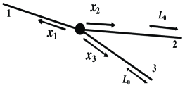
Figure 1: Three leads connected to an elastic scatterer

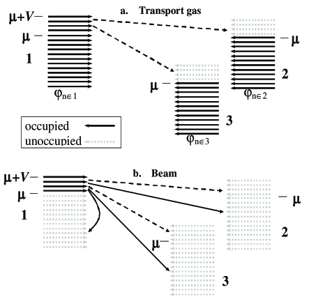
Figure 2: The occupations and possible transitions for $\omega>0$. Short horizontal arrows represent scattering states.

Following the ideas in neutron-scattering theory introduced by Van-HovevanHove we insert a complete set of eigenstates into Eq.(4) and get after a short manipulation:

$$S_{\alpha\beta}(\omega)=2\pi\sum_{f}\langle i|\hat{J}_{\alpha}(0)|f\rangle\langle f|\hat{J}_{\beta}(0)|i\rangle\delta(E_{i}-E_{f}-\omega),$$ (5)

where $E_{i}$ and $E_{f}$ are the energies of $|i\rangle$ and $|f\rangle$. The non-diagonal element $\langle i|\hat{J}_{\alpha}(0)|f\rangle$ is nonzero only if $|f\rangle$ differs from $|i\rangle$ by moving one particle from an occupied state, $\varphi_{n},$ to a previously unoccupied state, $\varphi_{n^{\prime}},$ i.e., $|f\rangle$ is of the form $\hat{a}_{n^{\prime}}^{{\dagger}}\hat{a}_{n}|i\rangle$ (up to a fermionic factor $c=\pm 1$, that will play no role below.) The term with the diagonal element $\langle i|\hat{J}_{\alpha}(0)|i\rangle$ which is the average current, $I_{\alpha}(V)$, on arm $\alpha$, yields a term $\sim\delta(\omega)$. In what follows we consider only $\omega\not=0$ and therefore neglect this term. In experiments the integration in Eq.(4) is limited by the sampling time of the experiment, $T_{s}$, and as a result $\delta(\omega)$ is smoothed into a peak with a width of $\simeq 1/T_{s}$ which means that the condition $\omega\not=0$ actually is $\omega T_{s}\gg 1$. We therefore have:

$$S_{\alpha\beta}(\omega)=2\pi\sum_{nn^{\prime}}J_{\alpha,nn^{\prime}}J_{\beta,nn^{\prime}}^{\ast}\delta(\epsilon_{n}-\epsilon_{n^{\prime}}-\omega),$$ (6)

where $J_{\alpha,nn^{\prime}}\equiv\langle i|\hat{J}_{\alpha}(0)\hat{a}_{n^{\prime}}^{{\dagger}}\hat{a}_{n}|i\rangle$, and where now the summation over $n$ and $n^{\prime}$ is over all single-particle states $\varphi_{n}$ and $\varphi_{n^{\prime}}$ which are occupied and unoccupied, respectively, in $|i\rangle$. The auto-correlator is

$$S_{\alpha\alpha}(\omega)=2\pi\sum_{nn^{\prime}}|J_{\alpha,nn^{\prime}}|^{2}\delta(\epsilon_{n}-\epsilon_{n^{\prime}}-\omega).$$ (7)

When the system is coupled to a measuring device (e.g., some circuit or an electro-magnetic field) through a small term linear in $\hat{J}_{\alpha}$, $S_{\alpha\alpha}(\omega)$ is a sum over single-particle transitions, the probability of each given by the Fermi golden rule, between an initial $\varphi_{n}$ and a final $\varphi_{n^{\prime}}$. (The cross-correlator, Eq.(6) for $\alpha\not=\beta$, should not be viewed similarly since then $J_{\alpha,nn^{\prime}}J_{\beta,nn^{\prime}}^{\ast}$ is not a transition amplitude squared). Via these transitions energy is transferred between the system and the measuring device: terms with $\epsilon_{n}>\epsilon_{n^{\prime}}$ (one particle goes down in energy) describe transitions in which an energy of $\omega=\epsilon_{n}-\epsilon_{n^{\prime}}>0$ is transferred from the system to the measuring device, while terms with $\epsilon_{n^{\prime}}>\epsilon_{n}$ (one particle goes up) describe transitions in which an energy of $-\omega=\epsilon_{n^{\prime}}-\epsilon_{n}>0$ is transferred from the measuring device to the system. When $\omega>0$, only the first type of terms will remain and $S_{\alpha\alpha}(\omega)$ will be the emission spectrum while $S_{\alpha\alpha}(-\omega)$ is the absorption spectrum. Thus we conclude that when $\alpha=\beta$ there will be emission of noise at frequency $\omega$ if and only if there exist occupied and unoccupied states in $|i\rangle,$ $\varphi_{n}$ and $\varphi_{n^{\prime}}$, with $|J_{\alpha,nn^{\prime}}|^{2}\not=0$ and $\omega=\epsilon_{n}-\epsilon_{n^{\prime}}>0.$ For $\alpha\not=\beta$, this is not necessarily so, since the terms in Eq.(6) are complex and may cancel.

Now let us compare the current and its fluctuations in the transport gas and the beam, considering the arms 2 and 3. The average currents in both systems are defined only by states in the energy window $[\mu,\mu+eV]$ and are the same: for $\beta=2,3$ one finds $I_{\beta}(V)=e^{2}T_{\beta}V/(2\pi)$ both for $|i\rangle=|beam\rangle$ and $|i\rangle=|transport\rangle$, where $T_{\beta}\equiv|s_{\beta 1}|^{2}$. (For simplicity we neglected the energy dependence of the transmission). By calculating the emission spectrum ($\omega>0$) we now show that the current fluctuations may differ. Rewriting Eqs.(6) and (7) for $\omega>0,$ taking into account the energy conservation and the different occupations in the states Eqs.(1) and (2), one has for the transport gas:

$$S_{\alpha\beta}^{tr}(\omega)=2\pi\sum J_{\alpha,nn^{\prime}}J_{\beta,nn^{\prime}}^{\ast}\delta(\epsilon_{n}-\epsilon_{n^{\prime}}-\omega)$$

$${}_{n\in 1,n^{\prime}\in 2,3}\ {}_{\mu<\epsilon_{n^{\prime}}<\epsilon_{n}<\mu+eV}\qquad\qquad\qquad$$ (8)

and for the beam:

$$S_{\alpha\beta}^{b}(\omega)=S_{\alpha\beta}^{tr}(\omega)+\sum_{n\in 1;\ \mu<\epsilon_{n}<\mu+\min(\omega,eV)}S_{\alpha\beta}^{(n)}(\omega).$$ (9)

Here $S_{\alpha\beta}^{(n)}(\omega)$ corresponds to the correlator in the state ${\hat{a}_{n}}^{{\dagger}}|vacuum\rangle$, which is a beam with a single particle, in a state $\varphi_{n}$:

$$S_{\alpha\beta}^{(n)}(\omega)=2\pi\sum_{n^{\prime}\in 1,2,3}J_{\alpha,nn^{\prime}}J_{\beta,nn^{\prime}}^{\ast}\delta(\epsilon_{n}-\epsilon_{n^{\prime}}-\omega).$$ (10)

$S_{\alpha\beta}^{tr}(\omega)$ contains transition amplitudes between occupied states in the energy window $[\mu,\mu+eV]$ to lower empty states inside the same energy window. These transitions, shown by dashed arrows in figs. 2a, and 2b, are possible both in the transport gas and the beam and therefore $S_{\alpha\beta}^{tr}(\omega)$ appears also in Eq.(9). Contrary to the first one, the second term in Eq.(9) contains transition amplitudes between occupied states in the energy window $[\mu,\mu+eV]$ to empty states below $\mu$ (long solid arrows in fig. 2b), transitions which are allowed only in the beam. Writing this term as a sum of single-particle correlators was possible since in the beam all the levels below $\mu$ are empty so the sum runs over all possible values of $n^{\prime}$ with a given energy, unlike in Eq.(8) for the transport gas where $n^{\prime}\notin 1$.

Now, the current matrix element is given by:

$$\langle i|\hat{j}_{\alpha}\;\hat{a}^{{\dagger}}_{n^{\prime}}\hat{a}_{n}|i\rangle=(c/2)\left[(k^{\prime}+k)e^{i(k-k^{\prime})x_{\alpha}}s_{\alpha 1}(k)^{\ast}\times\right.$$

$$\left.s_{\alpha\gamma^{\prime}}(k^{\prime})+(k^{\prime}-k)s_{\alpha 1}(k)^{\ast}\delta_{\alpha\gamma^{\prime}}e^{-i(k+k^{\prime})x_{\alpha}}\right]$$ (11)

for $n=(k,1)$ occupied and $n^{\prime}=(k^{\prime},\gamma^{\prime})$ empty. $c=\pm 1$, as above. Performing the average as defined in Eq.(3) and using the conditions for $L_{0}$, we obtain

$$J_{\alpha,nn^{\prime}}=(c/2)(k+k^{\prime})s_{\alpha 1}(k)^{\ast}s_{\alpha\gamma^{\prime}}(k^{\prime}).$$ (12)

This matrix element has no spatial dependence because the fast oscillating term in Eq.(Shot-noise in Transport and Beam Experiments) vanished while the slow oscillating one is constant within $L_{0}$. Inserting Eq. (12) into Eq.(6), transforming the sums over $k$ and $k^{\prime}$ into integrals, integrating using the condition $\omega,eV\ll\mu$, using the unitarity of the scattering matrix, $\sum_{\gamma}s_{\alpha\gamma}s_{\beta\gamma}^{\ast}=\delta_{\alpha\beta}$, one gets KhlusLesovikButtiker for $\alpha,\beta=2,3$, and $\omega>0$:

$$S_{\alpha\beta}^{tr}(\omega)=\frac{e^{2}}{2\pi}T_{\alpha}(\delta_{\alpha\beta}-T_{\beta})(eV-\omega)\theta(eV-\omega)$$ , (13)

where $\theta$ is the Heaviside step-function. Similarly, using Eq.(12) in Eq.(10) one gets for the single-particle correlator (see discussion below), for $\alpha,\beta=2,3$:

$$S_{\alpha\beta}^{(n)}(\omega)=\delta_{\alpha\beta}eI_{n,\alpha},$$ (14)

where $I_{n,\alpha}=eT_{\alpha}(k/m)(1/L)$ is the average current on arm $\alpha=2,3$ of a single particle in the state $n=(k,1)$.

Substituting Eq.(14) in Eq.(9), one gets for $\alpha,\beta=2,3$:

$$S_{\alpha\beta}^{b}(\omega)=S_{\alpha\beta}^{tr}(\omega)+\delta_{\alpha\beta}eI_{\alpha}(\omega),$$ (15)

where $I_{\alpha}(\omega)$ is the average current of the electrons in the energy window $[\mu,\mu+\min(\omega,eV)]$:

$$I_{\alpha}(\omega)\equiv\sum_{n\in 1;\ \mu<\epsilon_{n}<\mu+\min(\omega,eV)}I_{n,\alpha}=I_{\alpha}(V)\frac{\min(\omega,eV)}{eV}.$$ (16)

Eq.(15) is our main result and it demonstrates that although the average currents in arms 2 and 3 in the beam and the transport gas are the same, the current fluctuations in these arms generally differ. The beam has much more noise: e.g., for $\alpha=2,3$ the auto-correlation spectra of the transport state $S^{tr}_{\alpha\alpha}(\omega)$ has an upper cutoff at $\omega=eV$, but the auto-correlation spectra of the beam $S^{b}_{\alpha\alpha}(\omega)$ has no such cutoff. The spectra $S^{b}_{\alpha\alpha}(\omega)$ at $\omega>eV$ is given by the extra second term in in Eq.(15). Interestingly, this term is identical to the result for a beam of uncorrelated (Poissonian) classical particles S^n which carries an average current given by Eq.(16). Surprisingly, the cross-correlation, $S_{23}(\omega)$ is identical in the beam and the transport gas, since this term vanishes for $\alpha\not=\beta$.

According to Eq.(15) and Eq.(16) $S^{b}_{\alpha\alpha}(\omega)$ and $S^{tr}_{\alpha\alpha}(\omega)$ start to differ substantially for $\omega$ of order $eV$. The measurement in Ref. HBT electrons2, is consistent with Eq.(13) but since it is performed at $\omega\ll eV$, it can not distinguish between $S^{tr}_{\alpha\alpha}(\omega)$ and $S^{b}_{\alpha\alpha}(\omega)$. In Ref. HBT electrons, (see particularly Fig.3) it is claimed that the cross-correlation are measured in the time domain. The function that was obtained via this measurement has characteristic time-scale of $\sim 100ns$ which, in the frequency domain, corresponds to $10MHz$. However, in both Eq.(15) and Eq.(16) the only characteristic frequency scale is of the order of $eV\approx 10^{5}MHz$ (estimated for $\sim 30nA$ and transmission of order 1), that is many orders of magnitude larger. Thus, the results in Ref. HBT electrons, are not consistent with ours.

The simple case of a two-terminal device is obtained from the from Eq.(15) by taking $s_{13}=0$. In this case there is only one independent correlator, since $S_{11}(\omega)=S_{22}(\omega)=-S_{12}(\omega)\equiv S(\omega)$. All these correlators are different for the transport gas and the beam. Denoting $I$ as the average current in the device, one gets:

$$S^{b}(\omega)-S^{tr}(\omega)=eI\frac{\min(eV,\omega)}{eV},$$ (17)

We now explain the classical form of the extra term in Eq.(15). This term contains transition amplitudes from states in the energy window $[\mu,\mu+min(\omega,eV)]$ to states below $\mu$ (see the second term in Eq.(9) and Eq.(10)) . Since all final states are empty the quantum statistics plays no role. So, with no interactions and no statistics, the particles in this energy window are independent. For independent particles (classical or quantum), the correlator is a sum of their single-particle correlators: $S_{\alpha\beta}=\sum_{n}S_{\alpha\beta}^{(n)}$ (see the second term in Eq.(9) and Ref.S^n, ). Since the classical single-particle correlator is identical to its quantum counter-part according to Eq.(14) and Ref.S^n, , the contribution of the particles in the above energy window has a classical form.

It remains to understand why the quantum and classical single-particle correlators are equal. This is due to the averaging in Eq.(3), the unitarity of the scattering matrix and the assumption $\omega\ll\mu$. Here we will explain in detail only the role of the averaging in the vanishing of the cross-correlation: Before averaging, the single-particle temporal cross-correlator is

$$\langle\varphi_{1,k}|\hat{j}(x_{2},0)\hat{j}(x_{3},t)|\varphi_{1,k}\rangle=\frac{s_{21}s_{31}}{4L}e^{i\epsilon_{1,k}t}\times$$

$$e^{-ik(x_{2}-x_{3})}(-i\partial_{x_{2}}+k)(i\partial_{x_{3}}+k)\langle x_{2}|e^{-iHt}|x_{3}\rangle$$ (18)

where $|\varphi_{1,k}\rangle\equiv{\hat{a}_{1,k}}^{{\dagger}}|vacuum\rangle$, and where

$$\langle x_{2}|e^{-iHt)}|x_{3}\rangle=\frac{s_{23}}{\sqrt{2\pi t}}exp(-i\frac{(x_{2}+x_{3})^{2}}{2mt}+i\frac{\pi}{4})$$ (19)

is the (generally nonzero) propagator from $(x_{2},0)$ to $(x_{3},t)$, for $t>0$. For simplicity, we assume the $s_{\alpha,\beta}$’s are real and $k$-independent. The above correlator, Eq.(18), is generally different from zero (in contrast to its classical counter part). However, when applying the spatial averaging each of its terms becomes proportional to a new type of propagators: of a wave-packet around momentum $k>0$ which is localized in a segment of size $L_{0}$ around $x_{2}$ on arm 2 into a similar wave-packet around $x_{3}$ on arm 3. This is so because the factor $e^{-ik(x_{2}-x_{3})}\langle x_{2}|e^{-iHt}|x_{3}\rangle$ in Eq.(18) turns upon averaging into:

$$\left(\int_{L_{0}}\frac{dx_{2}}{L_{0}}e^{-ikx_{2}}\langle x_{2}|\right)e^{-iHt}\left(\int_{L_{0}}\frac{dx_{3}}{L_{0}}e^{ikx_{3}}|x_{3}\rangle\right)$$ (20)

where each integral is a wave-packet of the form described above. All the four terms in Eq.(18), become after averaging, proportional to propagators of similar though more complicated form. These propagators vanish in the limit $kL_{0}\gg 1$, causing the quantum single-particle cross-correlator of the average current to vanish, similarly to the classical one. This vanishing has a physical meaning: if a particle is at a point $x_{2}$ on arm 2 it has, due to Heisenberg-principle, large momentum uncertainty and thus, although it is already on arm 2, a possibility to return and be scattered into arm 3 and reach $x_{3}$. However, when it is spread out in a segment of size $L_{0}$ around $x_{2}$ which is much larger than the inverse of the average momentum, its momentum uncertainty is not enough to allow it to return, and therefore, as in the classical case, it is scattered into one arm, and remains in it. Comment: without imposing the unitarity, Eq.(19) would also contain terms $\sim exp[\pm i(x_{2}-x_{3})^{2}/(2mt)]$ that would yield generally nonzero contribution also after averaging.

To conclude, using the representation of the current noise as a sum over single-particle transitions we have shown that the current correlations in time and their spectra are different spatial in a transport and a beam experiment, although the average current is the same. Thus, the picture of current in a degenerate Fermi gas as a beam of particles with energies in the transport window is grossly over-simplified. For a three-terminal device, which is a solid state analog of a beam splitting setup (from arm 1 to arms 2 and 3), the difference is given by the second term in Eq.(15), which exists only in the beam, and which start to be important at $\omega$ of order of $eV$. In the range $\omega>eV$, where there is no noise in the transport gas, this extra term gives Poissonian white noise for the auto-correlators $S_{22}(\omega)$ and $S_{33}(\omega)$, but does not contribute to the cross-correlator $S_{23}(\omega)$.

This project was supported by the Israel Science Foundation, by the German-Israeli Foundation and by a joint grant from the Israeli Ministry of Science and the French Ministry of Research and Technology. We thank E. Comforti, B. Douçot, C. Glattli, M. Heiblum and D. Prober for instructive discussions. Some of this work was done while YI and UG were visiting the Ecole Normale Superieure in Paris. They acknowledge support by the Chaires Internationale Blaise Pascal.

References

- (1) V.A. Khlus, JETP 66, 1243 (1987); G.B. Lesovik, JETP Lett., 49, 592 (1989), M. Büttiker, Phys. Rev. B 46, 12485 (1992); S.-R. Yang, Solid State Commun., 81, 375 (1992).
- (2) M. Reznikov, M. Heiblum, H. Shtrikman, and D. Mahalu, Phys. Rev. Lett. 75, 3340 (1995). A. Kumar, L. Saminadayar, D. C. Glattli, Y. Jin and B. Etienne, Phys. Rev. Lett. 76, 2778 (1996).
- (3) A. A. Kozhevnikov, R.J. Schoelkopf and D.E. Prober, Phys. Rev. Lett. 84, 3398 (2000).
- (4) R. dePiccioto et al. Nature, 389, 162 (1997); L. Saminadayar et al. Phys. Rev. Lett. 79, 2526 (1997).
- (5) W. D. Oliver, J. Kim, R. C. Liu, Y. Yamamoto, Science 284, 299 (1999).
- (6) M. Henny, S. Oberholzer, C. Strunk, T. Heinzel, K. Ensslin, M. Holland, C. Schönenberger, Science 284, 296 (1999); S. Oberholzer et al., Physica E 6, 314 (2000).
- (7) T. Kodama et al., Phys. Rev. A 57, 2781 (1998).
- (8) W. Schottky, Annalen der Physik, 57, 541 (1918).
- (9) R.C. Liu, B. Odom, Y. Yamamoto and S. Tarucha, Nature 391, 263 (1998).
- (10) U. Gavish, Y. Levinson and Y. Imry, Phys. Rev. B 62, R10637 (2000). Y. Levinson and Y. Imry, in Proc. of the NATO ASI ”Mesoscope 99” in Ankara/Antalya, Kluwer 1999.
- (11) G. Lesovik and R. Loosen, JETP Lett., 65, 295 (1997).
- (12) L. van Hove, Phys. Rev 95, 249 (1954).
- (13) The single-particle classical correlator has the form Eq.(10) since a particle is scattered into arm 1 or 2 or 3 , so its cross-correlator vanishes while the auto correlation is the known Poissonian result. Formally: The classical current at a point on arm of a single particle incoming on arm 1 at velocity is: where is the particle distance from its initial point , and where or with probabilities and respectively. Now, . The first average is over scattering outcomes. The second is over . The particle is scattered only into one arm, so, . So, , where. is the average (time independent) current on arm . For a beam of independent particles one has: where is the total current.
- (14) Though not discussed here, the spatial correlations are also different in the transport gas and the beam.