How Irrelevant Operators affect the Determination of Fractional Charge

Abstract

We show that the inclusion of irrelevant terms in the hamiltonian describing tunneling between edge states in the fractional quantum Hall effect (FQHE) can lead to a variety of non perturbative behaviors in intermediate energy regimes, and, in particular, affect crucially the determination of charge through shot noise measurements. We show, for instance, that certain combinations of relevant and irrelevant terms can lead to an effective measured charge $\nu e$ in the strong backscattering limit and an effective measured charge $e$ in the weak backscattering limit, in sharp contrast with standard perturbative expectations. This provides a possible scenario to explain the experimental observations by Heiblum et al., which are so far not understood.

Recent experiments Comforti have raised the possibility that Laughlin quasiparticles (LQPs) Laughlin may be able to tunnel through very high barriers in a FQHE tunneling experiment if the beam of LQPs is diluted. This is unexpected. Conventional wisdom says instead that in the limit of strong pinching, the quantum Hall fluid is split into two pieces. The vicinity of this limit, if it can be described perturbatively, can only involve tunneling of electrons from one half to the other, and noise experiments should give an effective carrier charge equal to $e$. The experimental observations Comforti - an effective tunneling charge as low as $0.45e$ for a measured transparency of only $0.1$ - seems to be counterintuitive. Furthermore, unpublished experiments by Chung et al. ComfortiI revealed an effective tunneling charge $e$ for a full beam of LQPs incident on an almost open quantum point contact. Both of these surprising observations are so far not understood. In a recent work, Kane and Fisher KaneFisher02 investigated by a mix of perturbative and non perturbative techniques, the tunneling of diluted beams of LQPs in a set up similar to the one in Ref. Comforti , and found no evidence for the tunneling of LQPs through high barriers. In this letter, we consider, using techniques of integrable field theory, tunneling hamiltonians in a strongly non perturbative region, where irrelevant terms play a major role. We show that, as a result of strong interactions, it is in fact very possible to measure an effective tunneling charge $\nu e$ in a region of small transparency and $e$ in a region of high transparency, a result at odds with perturbative intuition. We use the electron charge as unit and set $h\equiv 1$ from now on.

Let us first recall the standard theoretical set-up for this problem. After bosonizing the chiral edges action, and performing some folding transformations, the hamiltonian with only the most relevant term included is the boundary sine-Gordon model KFold :

$$H={1\over 2}\int_{-\infty}^{0}\left[(\partial_{x}\phi)^{2}+\Pi^{2}\right]+v\cos\sqrt{2\pi\nu}\phi(0).$$ (1)

This model is integrable GhoZam , and DC current and noise can be calculated FLSI ; FLSII . In the weak backscattering limit, obtained at small $v$ or large energies, the backscattered current is small, and the noise is determined by incoherent tunneling of LQPs of charge $\nu$. On the other hand, in the strong backscattering limit, the transmitted current is small, and the noise is determined by incoherent tunneling of electrons. We exclusively consider the case of zero temperature, $T=0$, in this note. The exact solution of the hamiltonian relies crucially on an integrable quasiparticle description. At zero bias, $V=0$, the ground state of the theory is just the vacuum with neither kinks nor breathers; the quasiparticles are in fact defined as excitations above this vacuum. For $V>0$, kinks of charge unity start filling the vacuum. Unfolding the theory (1) gives rise to right moving particles only, and we parameterize their energy and momentum by $\epsilon=p=e^{\theta}$, $\theta$ the rapidity. The new ground state is made of kinks occupying the range $\theta\in(-\infty,A]$; in other words, the filling fractions are $f_{+}(\theta,V)=1$ for $\theta<A$ and $f_{+}(\theta,V)=0$ for $\theta>A$. The surface of the sea is approximately $A\approx\ln(V)$, but computing $A$ exactly requires some technology due to the kink interaction. There are no antikinks nor breathers in the sea at $T=0$, so their densities do not appear in this analysis. For ease of notation, we define $\rho(\theta)\equiv n_{+}(\theta,V)f_{+}(\theta,V)|_{T=0}$. At $T=0$ the quantization of allowed momenta reads:

$$2\pi\rho(\theta)=e^{\theta}+2\pi\int_{-\infty}^{A}\Phi(\theta-\theta^{\prime})\rho(\theta^{\prime})d\theta^{\prime},$$ (2)

where $\rho=0\hbox{ in }[A,\infty)$, and $\Phi={1\over 2i\pi}{d\over d\theta}S_{++}(\theta)$ follows from the kink-kink scattering matrix in the bulk. A straightforward exercise in Fourier transforms and Wiener Hopf integral equations FLSbig leads to $e^{A}={V\over 2}{G_{+}(0)\over G_{+}(i)}$, and thus,

$$\tilde{\rho}(\omega)={1\over 2i\pi}{G_{-}(\omega)G_{+}(i)\over\omega-i}e^{(i\omega+1)A}.$$ (3)

where the kernels have been defined as ($\gamma={1\over\nu}-1$)

$$G_{+}=\sqrt{2\pi(\gamma+1)}{\Gamma(-i(1+\gamma)\omega/2\gamma)\over\Gamma(-i\omega/2\gamma)\Gamma(1/2-i\omega/2)}e^{-i\omega\Delta},$$ (4)

and $G_{-}(\omega)=G_{+}(-\omega)$, $\Delta\equiv{1\over 2}\ln\gamma-{1+\gamma\over 2\gamma}\ln(1+\gamma)$.

It is important to stress that the quantization of the bulk theory (we neglect finite length effects here) is independent of the boundary interaction. The mere choice of the quasiparticle basis however does depend crucially on this interaction; in fact, it is chosen precisely in such a way that the quasiparticles scatter one by one, without particle production, on the boundary. This is described by a scattering matrix element $Q$, in terms of which the current reads FLSbig

$$I(V,T_{B})=\int_{-\infty}^{A}\rho(\theta)\left|Q\left(\theta-\theta_{B}\right)\right|^{2}d\theta$$ (5)

with $|Q|^{2}=1/(1+\exp[2(1-1/\nu)(\theta-\theta_{B})])$. Here, $\theta_{B}$ is a measure of the strength of the tunneling term in (1), $e^{\theta_{B}}\propto v^{1\over 1-\nu}$. Similarly, the noise can be written as

$$S(V,T_{B})=\int_{-\infty}^{A}\rho(\theta)\left(\left|Q\left(\theta-\theta_{B}\right)\right|^{2}-\left|Q\left(\theta-\theta_{B}\right)\right|^{4}\right)d\theta\;.$$ (6)

In terms of renormalization group theory (RG), the boundary interaction induces a flow from Neumann (N) to Dirichlet (D) boundary conditions. It is widely believed that these are the only possible conformal boundary conditions for the compact boson. The whole operator content at the strong backscattering (D) fixed point can be determined using general considerations of conformal invariance Affleck : the allowed operators have dimension $h_{D}=n^{2}/\nu$ modulo integers, where $n$ is an integer. We stress that there is no operator of dimension $\nu$ at this fixed point. Instead, the most relevant operator has $h=1/\nu$. This operator is $\cos\sqrt{2\pi/\nu}\tilde{\phi}$ ($\tilde{\phi}$ being the dual of the field $\phi$) and corresponds to transfer of charge unity.

The allowed operators at the weak backscattering (N) fixed point have dimensions $h_{N}=\nu m^{2}$ modulo integers, where $m$ is an integer. The tunneling of LQPs at this fixed point corresponds to $m=1$, and to the most relevant operator in its vicinity. Note that since $\nu$ is the inverse of an (odd) integer, the operator of dimension $h=1/\nu$ is allowed near this fixed point. This operator conforms to tunneling of a bunch of $1/\nu$ LQPs – in a sense an electron – in the weak backscattering limit.

The two types of tunneling charges can be identified theoretically and experimentally using the noise. Near the high energy fixed point, the noise as well as the backscattered current are due to rare tunnelings of LQPs, so $S\approx\nu(I_{0}-I)$, while near the low energy fixed point, the noise as well as the current are due to tunneling of electrons, so $S\approx I$. These results may appear to contradict the fact that in the integrable approach, the quasiparticles always have charge unity. What happens of course is that in the weak backscattering limit, these quasiparticles have non negligible probabilities of tunneling, so the term $|Q|^{4}$ is of the same order than $|Q|^{2}$, resulting into a slope $(-\nu)$.

Interestingly, hamiltonians with irrelevant terms added to the basic tunneling term in (1) are also solvable. Some technical points of such a model were already discussed in the case $\nu={1\over 2}$ in Ref. EKS , where the hamiltonian

$$H={1\over 2}\int_{-\infty}^{0}\left[(\partial_{x}\phi)^{2}+\Pi^{2}\right]+v_{1}\cos\sqrt{2\pi\nu}\phi(0)$$

$$+v_{2}\cos\sqrt{2\pi/\nu}\phi(0)+v_{3}\Pi(0)^{2}$$ (7)

was considered. Here, the $v_{1}$-term corresponds to tunneling of LQPs, the $v_{2}$-term to tunneling of electrons, and the $v_{3}$-term to an on-site density-density interaction on the constriction. The on-site density-density interaction reveals the reasonable assumption that electron forward scattering is stronger on the constriction than in the bulk. The basis of quasiparticles is the same as before, and it was shown in Ref. EKS that the only change is the boundary scattering matrix, which follows from

$$P+Q = i\coth\left({\theta-\theta_{B}^{3}\over 2}-{i\pi\over 4}\right)$$ (8)

$$P-Q = -i\tanh\left({\theta-\theta_{B}^{1}\over 2}-{i\pi\over 4}\right)\coth\left({\theta-\theta_{B}^{2}\over 2}-{i\pi\over 4}\right)$$

The relation between the bare parameters $v_{i}$ and the parameters in the scattering matrix $\theta_{B}^{i}$ is a bit complicated (it also depends on the regularization procedure adopted). However, it simplifies in the limit of small bare couplings where we find, up to irrelevant numerical factors, $v_{1}\propto e^{\theta_{B}^{1}/2}$, $v_{2}\propto\left(e^{-\theta_{B}^{2}}+e^{-\theta_{B}^{3}}\right)$, and $v_{3}\propto\left(e^{-\theta_{B}^{2}}-e^{-\theta_{B}^{3}}\right)$. In the case $\nu=1/2$, the particles have a trivial interaction in the bulk, so the density is simply $\rho=e^{\theta}$, and the Fermi momentum $e^{A}=V/2$. Assuming bare couplings are all rather small, we restrict to the regime $\theta_{B}^{1}<<\theta_{B}^{2},\theta_{B}^{3}$.

The interplay of the different terms can lead to several kinds of behaviors. We only discuss here the question of effective tunneling charges. Thus, the curves representing the noise $S/V$ as a function of the current $I/V$ are considered. With a single tunneling term, see Eq. (1), these curves have a single branch going from the origin to the point $I/V=\nu$. The most interesting feature of such a graph is its slope at the two extremities: near $I/V=0$ the slope is unity corresponding to tunneling of electrons, and near $I/V=\nu$ the slope is $(-\nu)$ corresponding to tunneling of LQPs with charge $\nu$.

If we include irrelevant terms under the choice that $\theta_{B}^{2}\approx\theta_{B}^{3}$, the results are similar to the ones obtained with a single tunneling term. This can be explicitely seen by considering a particle with energy $e^{\theta}$; the boundary conditions it will see depend on the magnitude of $\theta$, giving rise to two different energy domains:

$$\begin{array}[]{ccccccccc}&{}\hfil&\theta_{B}^{3}{}{}&\approx&~{}~{}\theta_{B}^{2}{}{}&\gg&~{}~{}\theta_{B}^{1}&{}\hfil&\cr&P\approx 0&{}\hfil&&{}\hfil&P\approx 0&{}\hfil&P\approx-i&\cr&Q\approx i&{}\hfil&&{}\hfil&Q\approx-i&{}\hfil&Q\approx 0&\cr&N&{}\hfil&&{}\hfil&N&{}\hfil&D&\end{array}$$ (9)

As the energy scale is increased - corresponding, for instance, to the increase of the applied voltage - the system successively sees D, then N boundary conditions, just like in the case with a single perturbation. Irrelevant terms do not have any strong qualitative effect.

It turns however out that things are quite different if there is a ‘resonance’ between the $\cos\sqrt{2\pi/\nu}\phi$ and $(\Pi)^{2}$ terms. This corresponds to $\theta_{B}^{3}\gg\theta_{B}^{2}\gg\theta_{B}^{1}$ (similar results are also obtained when $\theta_{B}^{2}\gg\theta_{B}^{3}\gg\theta_{B}^{1}$.) The meaning of the ‘resonance’ between the two irrelevant terms is not entirely clear: technically, it corresponds to having the term of dimension 2 being the regularized square of the bare tunneling term, as $\partial\cos\sqrt{\pi}\phi\cos\sqrt{\pi}\phi\propto\cos 2\sqrt{\pi}\phi+(\partial\phi)^{2}$. In that case, a variety of behaviors appears between the two energy scales $e^{\theta_{B}^{2}}$ and $e^{\theta_{B}^{3}}$ and strongly counterintuitive properties can be observed. If we consider again a particle with energy $e^{\theta}$, the boundary conditions it will see now fall within four energy domains:

$$\begin{array}[]{ccccccccc}&{}\hfil&\theta_{B}^{3}{}{}&\gg&~{}~{}\theta_{B}^{2}{}{}&\gg&~{}~{}\theta_{B}^{1}&{}\hfil&\cr&P\approx 0&{}\hfil&P\approx-i&{}\hfil&P\approx 0&{}\hfil&P\approx-i&\cr&Q\approx i&{}\hfil&Q\approx 0&{}\hfil&Q\approx-i&{}\hfil&Q\approx 0&\cr&N&{}\hfil&D&{}\hfil&N&{}\hfil&D&\end{array}$$ (10)

Consequently, as the energy scale is increased, the system successively sees D, then N, then D, then N boundary conditions.

In the presence of the three tunneling terms, and restricting to the situation $\theta_{B}^{3}\gg\theta_{B}^{2}\gg\theta_{B}^{1}$ , the current upon increasing the voltage increases from $0$ to a value very close to $I/V\approx\nu$, then goes back to a value very close to $I/V\approx 0$, then back to $I/V=\nu$. Only the two extremes are truly reached, and correspond to the fixed points that were mentioned before.

Of special interest are then the evolution of the noise, and especially the slopes of $S$ versus $I$ near the fixed points, as illustrated in Fig. 1.

Figure 1: Shot noise vs. current for $\nu=1/2$ and effective impurity strengths $(\theta_{B}^{1}=\ln(1.01))\ll(\theta_{B}^{2}=\ln(100))\ll(\theta_{B}^{3}=\ln(100000))$. The applied voltage $V$ is increased along the direction of the arrows on the ‘roaming trajectory’. Evidently, the effective charge exhibits changes as a function of the applied voltage.

Of course, a slope unity is observed at a real low energy $V\ll\theta_{B}^{1}$. In that case, all particles in the reservoir see D boundary conditions, $|Q|^{2}$ is always very small, $|Q|^{4}$ negligible compared to it. While the $N$ fixed point is initially approached with a slope $(-\nu)$ (corresponding to the tunneling of LQPs) it is left, as the voltage is increased, with a slope $(-1)$ instead of $(-\nu)$. This conforms to the tunneling process of $1/\nu$ LQPs from one edge to the other and was recently observed by Chung et al. ComfortiI .

As the voltage is increased ever further and the strong backscattering fixed point is approached again, the slope is equal to $\nu$ and not unity. In a naive perturbative analysis, one would study the vicinity of the strong backscattering fixed point and conclude that such a slope is not possible since there is no corresponding operator - physically, LQPs cannot tunnel ‘out’ of the quantum Hall fluid, where only electrons are known to exist. However, one should not forget that the strong backscattering fixed point is never actually reached on our trajectory - and presumably, what happens is that the slope $\nu$ cannot be understood perturbatively in the vicinity of that fixed point. Rather, in this case $\nu=1/2$, there are indications that the RG trajectory gets close to another fixed point, characterized by D boundary conditions with $\phi$ pinned to values $\phi(0)={2n\pi\over\sqrt{4\pi}}$. The slope $1/2$ could then be interpreted perturbatively in the limit of that fixed point. The situation bears some resemblance to the case of resonant tunneling discussed in Ref. KFold , where the slope would be interpreted as resulting from the tunneling of ‘half electrons’, that is (whole) electrons tunneling through an island. However, the situation is different here: the hamiltonian is not the resonant tunneling hamiltonian. For $\nu=1/2$, the resonant tunneling term $\cos 2\sqrt{2\pi\nu}\phi(0)$ is irrelevant and would not lead to the phenomena described above. Nevertheless, our findings might be interpreted in a way that the scattering potential effectively creates an ‘island’ at intermediate energy scales.

A drawback of the foregoing scenario is that, to observe the slope $\nu$ at fixed $\theta_{B}$’s, the strong backscattering limit has to be approached along an increasing voltage. This can easily be remedied however. One can for instance consider instead fixing $V$, and changing the $\theta_{B}$’s - corresponding to changing the backscattering potential in an experiment. Fig. 2 shows the noise and current for a particular trajectory where $\theta_{B}^{1}$ is increased while $\theta_{B}^{2}$ and $\theta_{B}^{3}$ are decreased.

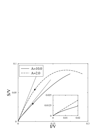
Figure 2: Shot noise vs. current for $\nu=1/2$ and fixed voltages. The effective impurity strengths are varied as $\theta_{B}^{1}=\theta$, $\theta_{B}^{2}=100-\theta$, and $\theta_{B}^{3}=1000-10\theta$ with $\theta\in[1.0,5.0]$. The inset zooms into the region of very strong backscattering.

This corresponds to increasing simultaneously the three scattering terms - hence, ‘pinching the point contact’. In that case, we find that, depending on the voltage, one can apparently approach the strong backscattering limit with a slope $\nu=1/2$. As emphasized in the inset of Fig. 2, in the very strong backscattering limit ($S/V,I/V\approx 0.005$) the slope $\nu=1/2$ reverts to a slope unity, the expected perturbative result. What we see is that, for an appropriate choice of parameters, the domain where this perturbative result can be observed is very small, while it is possible to get instead a slope $\nu=1/2$ over a large domain, and very close to the strong backscattering limit.

Although the foregoing results are obtained for $\nu=1/2$, they should reflect general properties of the field theory for all values of $\nu\leq{1\over 2}$, that is in the “attractive regime” of the boundary sine-Gordon model. We thus expect that these properties will be observed at all filling fractions $\nu={1\over t}$ with $t>1$ an odd integer. Since these are the filling factors, where chiral edge excitations are responsible for transport in real FQHE devices, the field theories (1) and (7) provide a valid description of the tunneling phenomena in such systems.

In any case, it is possible to carry out, to some extent, an analysis similar to the $\nu=1/2$ one for arbitrary $\nu$, based on the fact that the hamiltonian (7) is integrable. A minor difference is that we do not know the correspondence between the hamiltonian and the reflection matrix, which was afforded by the free fermion representation in the case $\nu=1/2$ . A more important difference is that, for $\nu<1/2$, the second cosine is not the least irrelevant one, which makes the integrable hamiltonian rather non generic. Now, for hamiltonian (7), general considerations ensure that the reflection matrix differs from the usual ones by CDD phase factors (that is, factors which preserve all the symmetries and physical properties of the scattering matrices GhoZam ), and therefore must have the general form (recall $\gamma={1\over\nu}-1$):

$$P+Q = -\exp\left[i\chi_{g}(\theta)\right]\coth\left({\theta-\theta_{B}^{3}\over 2}-{i\pi\over 4}\right)$$

$$P-Q = \exp\left[i\chi_{g}(\theta)\right]\tanh\left({\gamma(\theta-\theta_{B}^{1})\over 2}-{i\pi\over 4}\right)$$ (11)

$$\times \coth\left({\theta-\theta_{B}^{2}\over 2}-{i\pi\over 4}\right).$$

The transmission probability $|Q|^{2}$ can then be extracted from these expressions, and current and noise computed as for $\nu=1/2$. Similar results are observed, with the main difference that the slopes near the weak and strong backscattering limit are not restricted to unity and $\nu$ any longer: intermediate values can appear, cf. Fig. 3.

Figure 3: Shot noise vs. current for $\nu=1/3$ and fixed voltages. The effective impurity strengths are varied as $\theta_{B}^{1}=\theta$, $\theta_{B}^{2}=100-\theta$, and $\theta_{B}^{3}=1000-10\theta$ with $\theta\in[1.0,5.0]$. The inset zooms into the region of very strong backscattering.

Remarkably, slopes varying between $1/3$ and unity were observed in the noise experiments on FQHE devices at filling fraction $\nu=1/3$ in Ref. Comforti .

In conclusion, we have shown that the inclusion of irrelevant terms of a reasonable magnitude can lead to situations, where the effective charge extracted from the slope of the shot noise takes counterintuitive values. Although we have not precisely investigated the experimental scenario of diluted beams incident on a quantum point contact, our predictions could well be important to describe the so far unexplained experimental results in Ref. Comforti . We believe that at intermediate energies irrelevant operators are generally important. Therefore, non perturbative analyses are essential to interpret transport experiments at finite temperature and applied voltage.

We thank Y. C. Chung, R. Egger, H. Grabert, M. Heiblum, and C. L. Kane for helpful discussions. HS benefitted from the kind hospitality of the Freiburg Physics Department while this work was carried out, and was supported by the DOE and the Humboldt Foundation. BT was supported by the DFG and the LSF program.

References

- (1) E. Comforti, Y. C. Chung, M. Heiblum, V. Umansky, and D. Mahalu, Nature 416, 515 (2002).
- (2) R. B. Laughlin, Phys. Rev. Lett. 50, 1395 (1982).
- (3) Y. C. Chung, M. Heiblum, Y. Oreg, V. Umansky, and D. Mahalu, cond-mat/0304610; Y. C. Chung, private communications.
- (4) C. L. Kane and M. P. A. Fisher, Phys. Rev. B 67, 045307 (2003).
- (5) C. L. Kane and M. P. A. Fisher, Phys. Rev. B 46, 15233 (1992).
- (6) S. Ghoshal and S. Zamolodchikov, Int. J. Mod. Phys. A 9, 3841 (1994).
- (7) P. Fendley, A. W. W. Ludwig, and H. Saleur, Phys. Rev. Lett. 74, 3005 (1995).
- (8) P. Fendley, A. W. W. Ludwig, and H. Saleur, Phys. Rev. Lett. 75, 2196 (1995).
- (9) P. Fendley, A. W. W. Ludwig, and H. Saleur, Phys. Rev. B 52, 8934 (1995).
- (10) I. Affleck, “Conformal field theory approach to quantum impurity problems”, cond-mat/9311054, and references therein.
- (11) R. Egger, A. Komnik, and H. Saleur, Phys. Rev. B 60, R5113 (1999).