Glass transition in a simple stochasic model with back-reaction

Abstract

We formulate and solve a model of dynamical arrest in colloids. A particle is coupled to the bath of statistically identical particles. The dynamics is described by Langevin equation with stochastic external force described by telegraphic noise. The interaction with the bath is taken into account self-consistently through the back-reaction mechanism. Dynamically induced glass transition occurs for certain value of the coupling strength. Edwards-Anderson parameter jumps discontinuously at the transition. Another order parameter can be also defined, which vanishes continuously with exponent $1/2$ at the critical point. Non-linear response to harmonic perturbation is found.

1 Introduction

Glass transition and slow relaxation in systems characterised by weak ergodicity breaking remains still an open area, despite many efforts and numerous significant results in the last decade angell_95 ; pa_ste_ab_an_84 ; pa_me_dedo_85 ; ki_thi_87 ; ki_thi_87a ; ki_thi_wo_89 ; ritort_95 ; fra_he_95 ; cu_ku_93 ; fra_me_pa_pe_98 ; ba_bu_me_96a ; kurchan_92 ; cu_ku_95 ; ma_pa_ri_94b ; nieuwenhuizen_98 ; ca_gia_pa_99 ; ca_gia_pa_99a ; me_pa_99 ; co_pa_ve_00 ; cu_ku_pa_ri_95 ; par_sla_00 ; kaw_kim_01 . Among the host of diverse phenomena we are motivated here mostly by the effect of dynamical arrest in colloidal matter fie_sol_cat_99 ; fu_cat_03 ; cates_02 ; pue_fu_cat_02 ; fu_cat_02 ; zac_fof_daw_bul_sci_tar_02 ; law_rea_mcc_deg_tar_daw_02 ; sti_vla_lop_roo_mei_02 ; fab_got_sci_tar_thi_99 , observed experimentally and thoroughly investigated by numerical simulations and Mode-Coupling method. Below the transition point, the dynamics effectively leads to a glassy state with diverging viscosity, however the static thermodynamic transition may not be identifiable. Indeed, dynamical or structural arrest demonstrates the glass transition as a purely dynamic and self-consistent phenomenon, where casual slowdown of certain particles prevents some other particles from moving, which may slow down the others even more etc. The self-consistent nature of the phenomenon is reflected by the analytical approaches available now. One of the most striking phenomena in colloids, suspensions and granular matter is the non-Newtonian response to mechanical perturbation. On one hand, we can have shear-thinning, which amounts to a decrease if viscosity due to applied field, which can be interpreted as restoration of ergodicity due to perturbation cates_02 . On the other hand, increase of viscosity may result in shear thickening or even jamming, typically observed in particulate or granular matter cat_wit_bou_cla_99 ; ber_bib_sch_02 .

From the theoretical side, the Mode-Coupling (MC) equations provide us with a well-established framework, capable of explaining a good deal of experimental data gotze_91 ; go_sj_92 ; bouchaud ; sjogren_03 . The attempts to derive the MC equations starting from the Hamiltonian of the system were successful in the mean-field approximation. It was perhaps the $p$-spin spherical model ki_thi_87 ; ki_thi_87a ; ki_thi_wo_89 ; cu_ku_95 , where the machinery reached the farther edge of our current understanding of the phenomenon.

However, the bottom-up approach starting with writing explicit Hamiltonians is far from being complete. The presence of the reparametrisation invariance cu_ku_95 ; cu_ku_98 leaves the numerical solution of the MC equations as the only means for obtaining the true time-dependence of the correlation and response functions. Also the mean-field approximation generally used now seems to be very difficult to overcome.

The serious difficulties remaining in using the more advanced MC techniques leave the space for more simple phenomenological approaches. We want to follow this path in the present work.

Indeed, the mathematical substance of the Mode Coupling method can be summarised by saying that the time dependence of the correlation (and response) functions depends non-linearly and in time-delayed manner on these functions themselves. Actually, the memory kernel in the MC equations, which is primarily dictated by the properties of the reservoir, depends of the system dynamics.

We may represent the dynamics of the system by a stochastic process and the parameters of the process depend on time through the averaged properties of the process itself. In order to study generic properties of such problems it can be useful to establish a simple idealised model, which would capture the essential mathematic ingredients while avoiding the complications which arise from choosing a specific Hamiltonian at the beginning. The most important ingredient in such an idealised model should be the mechanism of the back-reaction.

We introduced recently chv_sla_02 a very simple stochastic process, in which the back-reaction leads to rich dynamic behaviour. The main characteristics was the presence of a phase transition from ergodic to non-ergodic phase. The principal aim of the present work is to investigate analytically some of the properties of the transition and from the numerical solution of the corresponding differential equations infer the non-trivial critical behaviour.

2 Langevin equation with back–reaction

2.1 System of coupled particles

The model system we will have in mind will be composed of particles, relaxing to their equilibrium positions under the influence of surrounding particles. They can be viewed as colloidal particles immersed in a solvent, but the formulation of our model is generic enough to allow for other interpretations as well, e. g. they can be viewed as micro-domains in a relaxor ferroelectric material.

The time evolution of the model can lead to dynamical arrest, where particles are locked in their positions by surrounding particles, which are also locked in their turn. Therefore, the dynamics can lead to the spatially disordered but time-stable stationary state with glass properties. The indication of the glass transition will be the non-zero value of the Edwards-Anderson order parameter and sensitivity to initial conditions. The interaction between particles will be taken into account on a phenomenological level; if we concentrate on a randomly selected particle (single relaxor), the external field from the rest of the system (reservoir) will change as the states of the other particles (relaxors in reservoir) evolve. The changes in the local external field will be the more rapid the faster is the evolution of the other particles. This leads to the idea of expressing the intensity of the changes in th external field through the velocity of movement of the relaxors in the reservoir. As we suppose all particles to be statistically identical, the movement of our single relaxor should be in probabilistic sense equivalent to the movement of any relaxor within the reservoir. This consideration closes the loop.

We will try to express the intensity of the changes of the local field through the averaged properties of the movement of the single relaxor itself. This introduces the idea of back-reaction: the probabilistic properties of the reservoir dictate the system evolution and the averaged system dynamics tunes the properties of the reservoir itself.

To be more specific, our single relaxor will be described by the continuous real stochastic variable ${\sf X}(t)$. It will evolve under influence of the environmental force, represented by the stochastic variable ${\sf Q}(t)$. The force will be modelled by a two–valued random process ${\sf Q}(t)\in\{-q,+q\}$ horsthemke , jumping at random instants. Occurrence of the jumps are governed by a self-exciting point process cox ; snyder with time-dependent intensity $\frac{1}{2}\lambda(t)$.

For given (friction-reduced) force ${\sf Q}(t)$ the single relaxor is described by the Langevin equation pomeau ; sibani ; morita

$$\frac{d}{dt}\,{\sf X}(t)=-\gamma\,{\sf X}(t)+{\sf Q}(t)$$ (1)

with initial conditions ${\sf X}(0)={\sf X}_{0}$ and ${\sf Q}(0)={\sf Q}_{0}$.

We may consider the process ${\sf X}(t)$ as a movement of an over-damped particle which slides in a parabolic potential well; the parabola jumps between two positions at random instants, with time-dependent rate $\frac{1}{2}\lambda(t)$.

The intensity of the process, or the frequency of jumps, $\frac{1}{2}\lambda(t)$, is related to the movement of the surrounding relaxors, considered as a reservoir. Intuitively the frequency must be smaller if the movement of the relaxors is slower. Therefore, the function $\lambda(t)$ should be coupled to the velocity ${\sf V}(t)=\frac{d}{dt}\,{\sf X}(t)$.

However, it is not obvious a priori what should be the specific functional dependence. We only require that the dependence is described by a non-negative function analytic at the origin. The simplest choice satisfying this property is

$$\lambda(t)=\epsilon\frac{\gamma}{q^{2}}\left\langle\,{\sf V}^{2}(t)\,\right\rangle$$ (2)

where $\epsilon$ is the dimensionless coupling strength parameter. The latter prescription is the form of the back-reaction we will study in the following. The model described above is sketched schematically in the Fig. 1.

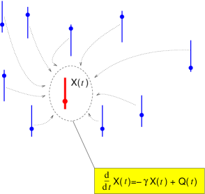
Figure 1: Schematical picture of our model. Relaxing particles in the reservoir influence the relaxation of the selected particle, described by the Langevin equation shown in the frame box.

The parameters $\gamma$ and $q$ can be in principle rescaled to 1 by appropriate choice of the units of time and length. Therefore, the coupling strength $\epsilon$ remains to be the only physically relevant parameter tuning the behaviour of the system. As we will see, there is a qualitative change in the behaviour of the system at a certain critical value of $\epsilon$.

2.2 Properties of the environmental force ${\sf Q}(t)$

The force ${\sf Q}(t)$ is a time-inhomogeneous Markov process, therefore its properties are fully described by a master equation. More specifically, let us define the probabilities

$$\pi_{\pm}(t)={\rm Prob}\left\{\,{\sf Q}(t)=\pm q\right\}$$ (3)

making the vector $\boldsymbol{\pi}(t)=\begin{pmatrix}\pi_{-}(t)\\ \pi_{+}(t)\end{pmatrix}$ which satisfies the Pauli master equation

$$\frac{d}{dt}\boldsymbol{\pi}(t)=-\frac{1}{2}\lambda(t)\left(\begin{array}[]{rr}1&-1\\ -1&1\end{array}\right)\boldsymbol{\pi}(t)\;.$$ (4)

Solving the equation amounts to calculation of the corresponding time-ordered exponential. The averages and correlation functions can be expressed through the integrated intensity

$$\Lambda(t)=\int_{0}^{t}\,\lambda(t^{\prime}){\rm d}t^{\prime}\;.$$ (5)

The time dependence of the vector $\boldsymbol{\pi}(t)$ can be written through the semi-group operator

$$R(t,t_{0})=\left(\begin{array}[]{rr}1&0\\ 0&1\end{array}\right)+\frac{1}{2}\left({\rm e}^{-\Lambda(t)+\Lambda(t_{0})}-1\right)\left(\begin{array}[]{rr}1&-1\\ -1&1\end{array}\right)$$ (6)

as $\boldsymbol{\pi}(t)=R(t,t_{0})\boldsymbol{\pi}(t_{0})$. Note that the semi-group operator obeys $R(t,\tau)R(\tau,t_{0})=R(t,t_{0})\;\forall\tau\in[t_{0},t]$ which testifies the Markov property of the process.

More explicitly, we find

$$\langle{\sf Q}(t)\rangle=\langle{\sf Q}_{0}\rangle\exp(-\Lambda(t))$$ (7)

$$\langle{\sf Q}(t){\sf Q}(t_{1})\rangle=q^{2}\exp(-|\Lambda(t)-\Lambda(t_{1})|)$$ (8)

Similarly, also the higher correlation functions can be written as products of exponentials with combinations of $\Lambda(t)$ with appropriate time arguments in the exponents. In fact, higher order correlation functions factorise into product of first and second order correlations, e. g.

$$\langle\prod_{l=1}^{2k}{\sf Q}(t_{l})\rangle=\prod_{l=1}^{k}\langle{\sf Q}(t_{2l}){\sf Q}(t_{2l-1})\rangle$$ (9)

for $t_{2k}\geq t_{2k-1}\geq...\geq t_{2}\geq t_{1}$. Another consequence is, that the cumulants of higher order than two vanish.

Note that the function $\Lambda(t)$ is non-decreasing and can either diverge (if $\lim_{t\to\infty}\lambda(t)>0$) or assume a finite limit for $t\to\infty$, if $\lambda(t)$ approaches 0 fast enough.

3 Glass transition and asymptotic relaxation

3.1 Equations for moments

For any given realisation of the process ${\sf Q}(t)$, the formal solution of Eq. (1) is

$${\sf X}(t)={\sf X}_{0}\,{\rm e}^{-\gamma t}+\int_{0}^{t}\,{\rm e}^{-\gamma(t-t^{\prime})}{\sf Q}(t^{\prime})\,{\rm d}t^{\prime}\quad.$$ (10)

If the function $\lambda(t)$ were known, various moments (and correlation functions) of the random process ${\sf X}(t)$ could have been computed from (10) using the expressions (7) and (8). However, in our case the function $\lambda(t)$ should be computed from the condition (2), relating it to the second moment of the time derivative of ${\sf X}(t)$. This suggests that sufficiently broad set of moments of ${\sf X}(t)$ and ${\sf V}(t)$ may provide a closed set of ordinary differential equations. The solution of this set will yield the closed description of the behaviour of our model.

Indeed, we can define four auxiliary functions

$$s_{1}(t) = {\rm e}^{-\Lambda(t)}$$ (11)

$$s_{2}(t) = {\rm e}^{-\gamma t}\int_{0}^{t}{\rm d}t^{\prime}\,{\rm e}^{\gamma t^{\prime}-\Lambda(t^{\prime})}\,$$ (12)

$$s_{3}(t) = {\rm e}^{-\gamma t-\Lambda(t)}\int_{0}^{t}{\rm d}t^{\prime}\,{\rm e}^{\gamma t^{\prime}+\Lambda(t^{\prime})}\,$$ (13)

$$s_{4}(t) = {\rm e}^{-2\gamma t}\int_{0}^{t}{\rm d}t^{\prime}\,{\rm e}^{\gamma t^{\prime}-\Lambda(t^{\prime})}\,\int_{0}^{t^{\prime}}{\rm d}t^{\prime\prime}\,{\rm e}^{\gamma t^{\prime\prime}+\Lambda(t^{\prime\prime})}$$ (14)

and express the requested quantities through these functions. For example the average coordinate can be written as

$$\langle{\sf X}(t)\rangle=\langle{\sf X}_{0}\rangle\,{\rm e}^{-\gamma t}+\langle{\sf Q}_{0}\rangle\,s_{2}(t)\;.$$ (15)

Similarly, the second moment of the coordinate is

$$\langle{\sf X}^{2}(t)\rangle=\langle{\sf X}^{2}_{0}\rangle\,{\rm e}^{-2\gamma t}+2\langle{\sf X}_{0}{\sf Q}_{0}\rangle\,{\rm e}^{-\gamma t}\,s_{2}(t)+2q^{2}\,s_{4}(t)\,.$$ (16)

The functions $s_{1}(t)$ to $s_{4}(t)$ can be found by solving the set of non-linear differential equations

$$\dot{s}_{1}(t) = -\lambda(t)\,s_{1}(t)$$ (17)

$$\dot{s}_{2}(t) = -\gamma\,s_{2}(t)+s_{1}(t)$$ (18)

$$\dot{s}_{3}(t) = 1-\left(\gamma+\lambda(t)\right)\,s_{3}(t)$$ (19)

$$\dot{s}_{4}(t) = -2\gamma\,s_{4}(t)+s_{3}(t)$$ (20)

with initial conditions $s_{1}(0)=1$, $s_{2}(0)=s_{3}(0)=s_{4}(0)=0$. The function $\lambda(t)$ occurring in the latter equations is itself a combination of the functions $s_{1}(t)$ to $s_{4}(t)$

$$\begin{split}\lambda(t)&=\epsilon\left[\gamma-2\gamma^{2}\,s_{3}(t)+2\gamma^{3}\,s_{4}(t)\right]+\\ &+\frac{\epsilon\gamma^{2}}{q^{2}}\left[\gamma\langle{\sf X}^{2}_{0}\rangle\,{\rm e}^{-2\gamma t}+2\gamma\langle{\sf X}_{0}{\sf Q}_{0}\rangle\,{\rm e}^{-\gamma t}\,s_{2}(t)-\right.\\ &\left.-2\langle{\sf X}_{0}{\sf Q}_{0}\rangle{\rm e}^{-\gamma t}\,s_{1}(t)\right]\quad.\end{split}$$ (21)

In the following we will assume that the initial condition of the stochastic process is ${\sf X}_{0}=0$ and $\langle{\sf Q}_{0}\rangle=0$, except explicitly mentioned cases. This lead to significant simplification of the mathematical structure of the equations. Indeed, the equations for $s_{3}(t)$ and $s_{4}(t)$ form a closed pair of equations

$$\begin{split}\dot{s}_{3}(t)=&1-(1+\epsilon)\gamma\,s_{3}(t)+\\ &+2\epsilon\gamma^{2}\,(s_{3}(t)-\gamma\,s_{4}(t))\,s_{3}(t)\\ \dot{s}_{4}(t)=&s_{3}(t)-2\gamma\,s_{4}(t)\quad.\end{split}$$ (22)

Unfortunately, the system (22) cannot be solved analytically. The best one can do is to transform the non-linear Ricatti-type set (22) to one differential equation of Abel type, whose solution, however, is not generally known. Therefore, we will solve the equations (22) numerically. Nevertheless, there is still a significant amount of information which can be extracted analytically.

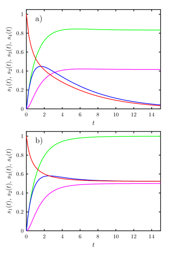
Figure 2: Time evolution of the auxiliary functions $s_{1}(t)$ (red line), $s_{2}(t)$ (blue line), $s_{3}(t)$ (green line), and $s_{4}(t)$ (magenta line) for $\gamma-1$, $q=1$. The panel a) corresponds to the value of the parameter $\epsilon=1.2$, while in the panel b) we have $\epsilon=0.8$.

The typical results of numerical solution are shown in figures 2 and 3. In Fig. 2 we can see the time evolution of the auxiliary functions $s_{1}(t)$ to $s_{4}(t)$. Fig. 3 shows the evolution of the switching rate $\lambda(t)$ and average coordinate $\langle{\sf X}(t)\rangle$ for non-zero value of the initial condition $\langle{\sf Q}_{0}\rangle$. We can observe qualitatively different behaviour for $\epsilon<1$ and $\epsilon>1$: first, the switching rate approaches a non-zero limit for $\epsilon>1$, while for $\epsilon<1$ it decays to zero. This means that in the latter case the system effectively freezes. This is further confirmed by the observation that for $\epsilon<1$ the limit value of the average coordinate depends on the initial conditions, while in the opposite case the dependence on initial conditions is lost for large times, the system equilibrates and the average coordinate converges always to zero. The following sections are mainly devoted to the analytical investigation of the above observations.

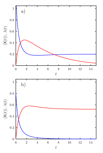
Figure 3: Time evolution of the average coordinate $\langle{\sf X}(t)\rangle$ computed for initial condition $\langle{\sf Q}_{0}\rangle=1$ (red line) and of the the switching rate $\lambda(t)$ (blue line) for $\gamma=1$, $q=1$. The panel a) corresponds to the value of the parameter $\epsilon=1.2$, while in the panel b) we have $\epsilon=0.8$.

3.2 Fixed points

The first step in investigating the behaviour of the system (22) is the search for the fixed points $[s_{3}^{*},s_{4}^{*}]$ of the dynamics. We found that there are only two fixed points, namely

$$[s_{3}^{*},s_{4}^{*}]=[\frac{1}{\gamma\epsilon},\frac{1}{2\gamma^{2}\epsilon}]$$ (23)

and

$$[s_{3}^{*},s_{4}^{*}]=[\frac{1}{\gamma},\frac{1}{2\gamma^{2}}]\quad.$$ (24)

Let us denote $\lambda_{\infty}$ the value of $\lambda(t)$ calculated at the corresponding fixed point. Using (21) the fixed point (23) yields $\lambda_{\infty}=(\epsilon-1)\gamma$ and the fixed point (24) yields $\lambda_{\infty}=0$.

The linear stability analysis reveals that for $\epsilon>1$ the fixed point (23) is stable, while (24) is unstable. On the other hand, for $\epsilon<1$ the fixed point (24) is stable, while (23) is unstable. The case $\epsilon=1$ is a marginal one, where both fixed points have one of the eigenvalues equal to 0. Therefore, the value $\epsilon=1$ marks a transition, whose nature will be further pursued in the following.

3.3 Ergodic regime $\epsilon>1$

In this case the relevant fixed point is (23) and inserting its value to the expressions for the moments of ${\sf X}(t)$ we find that both the average coordinate and the average velocity relaxes to zero. On the other hand, the fluctuations of the coordinate reach positive value, so

$$\begin{split}\lim_{t\to\infty}\langle{\sf X}(t)\rangle&=0\\ \lim_{t\to\infty}\langle{\sf X}^{2}(t)\rangle&=\frac{q^{2}}{\gamma^{2}\epsilon}\quad.\end{split}$$ (25)

The external force switching rate converges to positive constant $\lim_{t\to\infty}\lambda(t)=\gamma\,(\epsilon-1)$. In all cases the quantities of interest converge exponentially to their limit values The rate of convergence is determined by the lowest in absolute value eigenvalue, which is

$$\mu_{1}=-\frac{\gamma}{2}\left(\epsilon-\sqrt{\epsilon^{2}-8\epsilon+8}\right)\;.$$ (26)

In the interval $\epsilon\in(4-2\sqrt{2},4+2\sqrt{2})$ the eigenvalue acquires a non-zero imaginary part, which means that oscillatory behaviour is superimposed over the exponential relaxation.

The overall picture is the following. The back-reaction leads to self-adjustment of the switching rate of the external force exerted by the reservoir. The coordinate fluctuates around the origin and these fluctuations are stationary. Therefore, the stationary regime of the system corresponds to the primitive version with fixed $\lambda$, except the fact that the value of $\lambda$ is not given from outside, but tuned by the dynamics itself. We call this regime ergodic, because the particles do not freeze at some value of the coordinate ${\sf X(t)}$ but fluctuate forever.

The probability density for the coordinate

$$P(x,t)=\frac{\rm d}{{\rm d}x}{\rm Prob}\{{\sf X}(t)\leq x\}$$ (27)

approaches for $t\to\infty$ the function chv_sla_02 ; morita

$$\lim_{t\rightarrow\infty}P(x,t)=\frac{\gamma}{q}\,\frac{(1-\widetilde{x}^{2})^{(\epsilon-3)/2}}{B\left(\frac{\epsilon-1}{2},\frac{1}{2}\right)}\,\,\Theta(1-\widetilde{x}^{2})\,\,,$$ (28)

where $\widetilde{x}=x\gamma/q$, $\Theta(a)$ is the Heaviside unit-step function, and $B(a,b)$ denotes the Beta-function abramowitz . We can observe a qualitative change at the value $\epsilon=3$. For $\epsilon>3$ the limiting distribution (28) has a maximum for $x=0$ and approaches $0$ at the edges of the support $[-q/\gamma,q/\gamma]$, while for $\epsilon<3$ it has a minimum at $x=0$ and diverges at the edges of the support. The tendency for accumulating the probability close to the points $\pm q/\gamma$ when $\epsilon$ decreases can be regarded as a precursory phenomenon of the transition to the non-ergodic regime, investigated in the next sub-section.

3.4 Non-ergodic regime $\epsilon<1$

In this case we have (24) as stable fixed point. For $\langle{\sf Q}_{0}\rangle=0$ the average coordinate converges to 0 again, but the second moment approaches the $\epsilon$-independent maximum value

$$\lim_{t\to\infty}\langle{\sf X}^{2}(t)\rangle=\frac{q^{2}}{\gamma^{2}}\;.$$ (29)

As the probability density for the coordinate $P(x,t)$ has support limited to the interval $[-q/\gamma,q/\gamma]$, it follows from (29) the the limiting probability density is composed of two $\delta$-functions of equal weight $\frac{1}{2}$ located at the edges of the latter interval. More generally, for non-symmetric initial condition for the noise, $\langle{\sf Q}_{0}\rangle\neq 0$, the limiting probability density is the sum of two $\delta$-functions,

$$\lim_{t\to\infty}P(x,t)=\rho_{+}\,\delta\left(x-\frac{q}{\gamma}\right)+\rho_{-}\,\delta\left(x+\frac{q}{\gamma}\right)$$ (30)

the weights of which depend non-trivially on $\epsilon$ and the initial condition

$$\rho_{\pm}=\frac{1}{2}\left(1\pm\frac{\langle{\sf Q}_{0}\rangle}{q}\sigma(\epsilon)\right)$$ (31)

where $\sigma(\epsilon)=\lim_{t\to\infty}s_{1}(t)$.

The function $\lambda(t)$ relaxes to zero. Therefore, in this regime, the switching of the external force asymptotically stops and the coordinate ${\sf X}(t)$ approaches either the value $+q/\gamma$ or $-q/\gamma$, where it freezes. So, the coordinate acquires a random but time-independent asymptotic value. More precisely, the mean coordinate $\langle{\sf X}(t)\rangle$ approaches a generally non-zero asymptotic value, which depends on the initial condition. This is the manifestation of glassy state in the regime $\epsilon<0$, characterised by broken ergodicity and non-zero Edwards-Anderson order parameter. This point will be discussed more in detail later in the presentation of correlation functions.

As in the ergodic phase, all quantities relax toward their limit values exponentially for large times. The rate of convergence is governed by the eigenvalue with smallest modulus, which is now

$$\mu_{1}=-2\gamma(1-\epsilon)\;.$$ (32)

Note that, contrary to the ergodic regime, the eigenvalue is always a real number, so no oscillations occur, at least in the linearised approximation.

3.5 Marginal case $\epsilon=1$

Let us proceed by approaching the marginal case $\epsilon=1$ from the non-ergodic side, i. e. from below. It might be instructive to cast the equations (22) in terms of the eigenmodes of the linearised approximation. Namely, we can introduce the functions

$$\begin{split}\xi(t)&=\frac{1}{(2\epsilon-1)\gamma}\left(s_{3}(t)-\gamma\,s_{4}(t)-\frac{1}{2\gamma}\right)\\ \eta(t)&=\frac{1}{(2\epsilon-1)\gamma}\left(-s_{3}(t)+2\epsilon\gamma\,s_{4}(t)+\frac{1-\epsilon}{\gamma}\right)\end{split}$$ (33)

and express the equations (22) in the form

$$\begin{split}\dot{\xi}&=-2\gamma(1-\epsilon)\,\xi+2\epsilon\gamma^{3}(2\epsilon\,\xi+\eta)\,\xi\\ \dot{\eta}&=-\gamma\,\eta-2\epsilon\gamma^{3}(2\epsilon\,\xi+\eta)\,\xi\end{split}$$ (34)

The function $\xi(t)$ has a straightforward physical interpretation: it describes the time evolution of the switching rate of the external force. Indeed, inserting (33) into (21) we get

$$\lambda(t)=2\gamma^{3}(1-2\epsilon)\,\xi(t)\;.$$ (35)

The equations (34) are a convenient starting point for the investigation of the marginal regime. Taking $\epsilon=1$, the linear term in the equation for $\dot{\xi}$ vanishes, while the linear term in the equation for $\dot{\eta}$ remains. This suggests that in the long-time regime the value of $\eta$ will be negligible compared to $\xi$. This consideration will yield the leading term in the relaxation.

Thus, supposing $|\eta|\ll|\xi|$ we get the following approximate equation for $\xi$

$$\dot{\xi}=4\gamma^{3}\,\xi^{2}$$ (36)

which leads to the following asymptotic behaviour

$$\xi(t)\simeq-\frac{1}{4\gamma^{3}}\,\frac{1}{t}\quad,\;t\to\infty\quad.$$ (37)

Now we must check the assumption that $\eta$ is negligible compared to $\xi$. However, from (34) we can see that the leading term in the relaxation of $\eta$ is

$$\eta(t)\simeq\frac{1}{\gamma}\,\frac{1}{t^{2}}\quad,\;t\to\infty$$ (38)

and the assumption is therefore consistent.

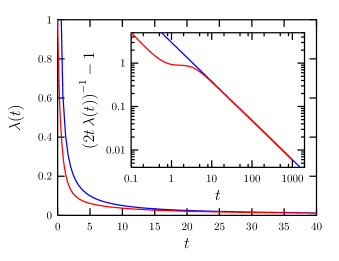
Figure 4: Time evolution of the switching rate in the marginal regime $\epsilon=1$, for $\gamma=1$, $q=1$. The red line is the numerical solution, blue line the asymptotic analytical solution (39). In the inset the deviation from the expression (39) is shown (red line). The blue line is power dependence $3\times\,t^{-0.9}$.

The consequence to draw is that in the marginal regime the relaxation becomes power-law with exponent $-1$. Especially, the relaxation of the switching rate follows the behaviour

$$\lambda(t)\simeq\frac{1}{2t}\quad,\;t\to\infty\;.$$ (39)

In Fig. 4 we can compare the numerical solution with the asymptotic behaviour (39). We can see not only that that the function $\lambda(t)$ approaches zero according to the power decay (39), but also the corrections to the asymptotic behaviour can be well approximated by a power. Indeed, from the inset in Fig. 4 we can see that

$$\frac{1}{2t\,\lambda(t)}-1\simeq 3\,t^{-0.9}\quad,\;t\to\infty\;.$$ (40)

It is interesting to note that the power in the correction is not an integer, so the naive expansion of the solution in powers of $t^{-1}$ cannot be used here. Instead, the behaviour (40) suggests the expression in the form of a continued fraction

$$\lambda(t)=\cfrac{1}{a_{1}t^{\alpha_{1}}+\cfrac{1}{a_{2}t^{\alpha_{2}}+\cfrac{1}{a_{3}t^{\alpha_{3}}+\dotsb}}}$$ (41)

where the values $a_{1}=2$ and $\alpha_{1}=1$ are known exactly and the next pair of parameters is estimated from the numerical solution as $a_{2}\simeq 1/6$ and $\alpha_{2}\simeq 0.9$.

4 Correlation functions

Additional information on the properties of the transition from ergodic to non-ergodic behaviour which occurs at the value $\epsilon=1$ can be gained from the two-time correlation functions. Let us have $t>t_{1}>0$ and define the correlation function

$$C(t,t_{1})=\langle{\sf X}(t){\sf X}(t_{1})\rangle\;.$$ (42)

It can be expressed through the functions $s_{1}(t)$ to $s_{4}(t)$. The most general formula is

$$\begin{split}C(t,t_{1})&=\langle{\sf X}_{0}\,\rangle{\rm e}^{-\gamma(t+t_{1})}+\\ &+\langle{\sf X}_{0}{\sf Q}_{0}\rangle\left[{\rm e}^{-\gamma t_{1}}\,s_{2}(t)+{\rm e}^{-\gamma t}\,s_{2}(t_{1})\right]+\\ &+q^{2}\biggl{[}2{\rm e}^{-\gamma(t-t_{1})}\,s_{4}(t_{1})+\\ &+\left(\,s_{2}(t)-{\rm e}^{-\gamma(t-t_{1})}\,s_{2}(t_{1})\right)\frac{s_{3}(t_{1})}{s_{1}(t_{1})}\biggr{]}\end{split}$$ (43)

although we suppose throughout this section that ${\sf X}_{0}=0$.

We show in figures 5 (ergodic regime) and 6 (non-ergodic regime) the evolution of correlation functions using the numerical solution for $s_{1}$ to $s_{4}$. We can observe the damping of the correlations in the ergodic regime, while in the non-ergodic regime the correlations converge to a finite limit. Let us now turn to the analytic investigation of the long-time behaviour of the correlation function.

For long enough times we can suppose that we are in the regime of exponential asymptotic relaxation of the functions $s_{1}(t)$ to $s_{4}(t)$ and $\lambda(t)$, which is governed by the eigenvalue closest to 0, as given by (26) and (32).

Let us start with the ergodic regime $\epsilon>1$. We find that for both $t\to\infty$ and $t_{1}\to\infty$ the correlation function behaves like

$$\begin{split}C(t,t_{1})\simeq\frac{q^{2}}{\gamma^{2}\epsilon(2-\epsilon)}&\left[{\rm e}^{-\gamma(\epsilon-1)(t-t_{1})}-\right.\\ &\left.-(\epsilon-1){\rm e}^{-\gamma(t-t_{1})}\right]\;.\end{split}$$ (44)

Important feature of this result is that the correlation in asymptotic regime depends only on the time difference $t-t_{1}$ and decays to zero when this difference increases. This supports the picture of the $\epsilon>1$ phase as a usual ergodic regime without long-time correlations.

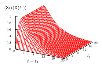
Figure 5: Correlation function in the ergodic regime, for $\epsilon=1.2$, $\gamma=1$, $q=1$.

The situation is dramatically different for $\epsilon<1$. Technically speaking, it is important that the function $\Lambda(t)$ has a finite limit for large times, $\lim_{t\to\infty}\Lambda(t)=\Lambda_{\infty}<\infty$. For $\epsilon$ close to $1$ (i. e. $1-\epsilon\ll 1$) the approach to this limit value can be written in the form

$$\Lambda(t)\simeq\Lambda_{\infty}-\theta\,{\rm e}^{-2\gamma(1-\epsilon)\,t}$$ (45)

where $\theta$ is a constant depending on $\epsilon$.

For large times the correction will be small and we can formally write the correlation function as expansion in powers of $\theta$. However, we should bear in mind that it is not $\theta$ itself, which is small, but the factor ${\rm e}^{-2\gamma(1-\epsilon)\,t}$ which appears always together with $\theta$.

Finally,

$$\begin{split}C(t,t_{1})&\simeq\frac{q^{2}}{\gamma^{2}}+\frac{\theta q^{2}}{(\gamma-\mu)\gamma}\left({\rm e}^{-\mu\,t}-{\rm e}^{-\mu\,t_{1}}\right)-\\ &-\frac{2\theta q^{2}\mu}{(\gamma-\mu)(2\gamma-\mu)\gamma}{\rm e}^{-\gamma(t-t_{1})-\mu\,t_{1}}+O(\theta^{2})\end{split}$$ (46)

using $\mu=2\gamma(1-\epsilon)$ for shorter notation.

We can see that the qualitative difference from the ergodic regime consists in the fact that for $\epsilon<1$ the correlation function converges to a positive $\epsilon$-independent constant $q^{2}/\gamma^{2}$. If we define the Edwards-Anderson order parameter

$$q_{\rm EA}=\lim_{\tau\to\infty}\lim_{t_{1}\to\infty}C(t_{1}+\tau,t_{1})$$ (47)

we can see that $q_{\rm EA}$ jumps discontinuously from the value $q_{\rm EA}=0$ for $\epsilon>1$ to $q_{\rm EA}=q^{2}/\gamma^{2}$ for $\epsilon<1$. This observation represents another evidence that there is a transition from ergodic regime to non-ergodic glassy regime at $\epsilon=1$. As the Edwards-Anderson parameter is discontinuous at the critical point, the transition should be classified as first-order from this point of view. However, because we do not deal with an equilibrium transition and the phenomenon is of purely dynamical origin, the canonic classification of phase transition as first or second order is of limited relevance here.

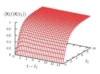
Figure 6: Correlation function in the non-ergodic regime, for $\epsilon=0.8$, $\gamma=1$, $q=1$.

5 Critical behaviour at $\epsilon\to 1^{-}$

We have already seen that it is possible to characterise the glass transition at $\epsilon=1$ through the Edwards-Anderson order parameter $q_{\rm EA}$. It has discontinuity at the transition, so the corresponding critical exponent is 0. Here we investigate another quantity, which can play the role of an order parameter, being zero in the ergodic and non-zero in the non-ergodic phase.

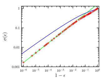
Figure 7: The critical behavior at $\epsilon\to 1$. Points ($+$) are results of numerical integration. The green line is the approximation (55), while the blue line is the exact upper bound $\sigma_{\rm upper}(\epsilon)$ given by formula (54).

The quantity in question will describe how the initial conditions affect the asymptotic vale of the average coordinate. We have already touched this point in Sec. 3.4. Up to now we assumed that the initial condition for the noise is such that $\langle{\sf Q}_{0}\rangle=0$. This assumption has the consequence that both in ergodic and non-ergodic regime the average coordinate converges to $0$. In this section we investigate the case $\langle{\sf Q}_{0}\rangle\neq 0$.

From (15) and (18)we can see that

$$\lim_{t\to\infty}\langle{\sf X}(t)\rangle=\frac{\langle{\sf Q}_{0}\rangle}{\gamma}\,\sigma(\epsilon)$$ (48)

where we defined, as in Sec. 3.4,

$$\sigma(\epsilon)=\lim_{t\to\infty}s_{1}(t)$$ (49)

stressing explicitly the dependence on $\epsilon$. The equations (22) hold also in case $\langle{\sf Q}_{0}\rangle\neq 0$. Therefore, we can proceed without further complications. We only need to plug the solution obtained the same way as in the sections 3 and 4 into the definition (11) of the function $s_{1}(t)$ and find the limit (49).

Let us first present the results of numerical integration. We will turn to the analytic estimate afterwards. The Fig. 7 shows the results of numerical integration, indicating that asymptotically for $\epsilon\to 1$ the behaviour follows the power law

$$\sigma(\epsilon)\sim(1-\epsilon)^{\frac{1}{2}}\;.$$ (50)

The exponent $1/2$ is still observed only empirically and we do not possess any proof that this is the exact value.

However, we may get some analytical argument in favour of this type of behaviour from the equations (19), (20), and (21), which can be rewritten in slightly different form. Defining new function $\psi(t)=s_{3}(t)-1/\gamma$ we can write the set of equations for the pair $\psi(t)$ and $\lambda(t)$

$$\begin{split}\dot{\psi}&=-\gamma\,\psi-\frac{1}{\gamma}\,\lambda-\lambda\psi\\ \dot{\lambda}&=-2\gamma(1-\epsilon)\,\lambda+2\epsilon\gamma^{2}\,\lambda\psi\end{split}$$ (51)

with initial conditions $\psi(0)=-1/\gamma$, $\lambda(0)=\epsilon\gamma$. If we further define $\Lambda_{\infty}=\int_{0}^{\infty}\lambda(t){\rm d}t$ and $\Psi_{\infty}=\int_{0}^{\infty}\psi(t){\rm d}t$, we can integrate both LHS and RHS of the equations (51) and obtain the exact relation between $\Lambda_{\infty}$ and $\Psi_{\infty}$

$$\epsilon=-2\Lambda_{\infty}-2\epsilon\gamma^{2}\,\Psi_{\infty}\;.$$ (52)

Knowing $\Lambda_{\infty}$ would solve the problem, because $\sigma(\epsilon)={\rm e}^{-\Lambda_{\infty}}$. However, in addition to (52) we need some other condition. It can be established from the observation that the equation for $\lambda(t)$ can be formally solved in the form

$$\lambda(t)=\epsilon\gamma\,\exp\left(-2\gamma(1-\epsilon)\,t+2\epsilon\gamma^{2}\int_{0}^{t}\psi(t^{\prime}){\rm d}t^{\prime}\right)\;.$$ (53)

and because $\psi(t)<0$, we have $\int_{0}^{t}\psi(t^{\prime}){\rm d}t^{\prime}>\Psi_{\infty}$. Therefore, we can write the following upper bound

$$\sigma(\epsilon)<\exp\left(-\frac{1}{2}W_{\rm L}\left(\frac{\epsilon\,{\rm e}^{-\epsilon}}{1-\epsilon}\right)\right)\equiv\sigma_{\rm upper}(\epsilon)$$ (54)

where $W_{\rm L}(x)$ is the Lambert function defined by the equation $W_{\rm L}(x)\,{\rm e}^{W_{\rm L}(x)}=x$.

The leading term in the asymptotic behaviour of the Lambert function for large argument is $W_{\rm L}(x)\simeq\ln x$. If we use it as an approximation for calculating the asymptotic behaviour of $\sigma(\epsilon)$, starting with (54) we finally get

$$\sigma(\epsilon)\simeq\sqrt{\rm e}\,\sqrt{1-\epsilon}$$ (55)

which is compatible with the behaviour (50). Actually, we can see in the Fig. 7 that the approximation (55) fits very well the results from numerical integration and lies much closer than the exact upper bound (54). Thus, we conjecture that the formula (55) is in fact the correct asymptotic behaviour for $\epsilon\to 1$.

To sum up, in the regime $\epsilon>1$, the initial conditions are irrelevant for long-time dynamics, as expected in the ergodic phase. On the other hand, for $\epsilon<1$, we observe that the asymptotic value of the average coordinate depends on the initial condition for the noise, which is yet another signature of ergodicity breaking. The factor $\sigma(\epsilon)$ measures the sensitivity to initial conditions: it vanishes in ergodic phase but remains non-zero in non-ergodic phase. So, it may be considered as a kind of order parameter. Close to the critical point $\epsilon=1$ it approaches zero continuously as a power with critical exponent $1/2$.

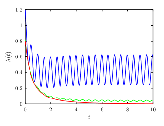
Figure 8: Response of the switching rate to harmonic external driving force for $\gamma=1$, $q=1$, $\epsilon=0.8$, $\omega=2\pi$ and $F_{0}=0.7$ (blue line) and $F_{0}=0.15$ (green line). The red line  shows the time dependence in absence of the external driving force.

6 Response to harmonic perturbation

Let us investigate now the response of the particle to the external driving force. Adding the additional term $F(t)=F_{0}\cos(\omega t)$ at the right hand side of Eq. (1), one can repeat, mutatis mutandis, all steps leading to the system of equations for the functions $s_{1}(t)$ to $s_{4}(t)$. We find that the equations (17)-(20) hold unchanged, while the influence of the external force modifies the expression (21) for $\lambda(t)$. Actually, in the present case one gets

$$\begin{split}\frac{\lambda(t)}{\epsilon\gamma}&=1-2\gamma\,s_{3}(t)+2\gamma^{2}\,s_{4}(t)+\\ &+\frac{1}{q^{2}}\left(\gamma\,{\rm e}^{-\gamma t}\int_{0}^{t}F(t^{\prime})\,{\rm e}^{\gamma t^{\prime}}\,{\rm d}t^{\prime}-F(t)\right)^{2}\quad.\end{split}$$ (56)

We assumed $\langle{\sf Q}_{0}\rangle=0$ and $\langle{\sf X}_{0}\rangle=0$ here.

First quantity to study is the response of the average coordinate. We find

$$\begin{split}\langle{\sf X}(t)\rangle=&\langle{\sf Q}_{0}\rangle\,{\rm e}^{-\gamma t}\int_{0}^{t}{\rm e}^{-\Lambda(t^{\prime})+\gamma t^{\prime}}\,{\rm d}t^{\prime}+\\ &+{\rm e}^{-\gamma t}\int_{0}^{t}F(t^{\prime})\,{\rm e}^{\gamma t^{\prime}}\,{\rm d}t^{\prime}\quad.\end{split}$$ (57)

Obviously enough, in the stationary regime the average coordinate oscillates around $0$ with the same frequency as the driving force $F(t)$. We arrive at the standard Debye-type dynamic susceptibility

$$\chi(t-t^{\prime})=\Theta(t-t^{\prime}){\rm e}^{-\gamma(t-t^{\prime})}\quad.$$ (58)

Thus, the exact response in terms of the coordinate is linear. This behaviour also does not depend on the value of $\epsilon$.

The situation becomes much more complicated when we turn to quantities, which depend non-linearly on the coordinate, especially the switching rate $\lambda(t)$. We solved numerically the set of equations (17) to (20) and (56). We can see in Fig. 8 the evolution of the function $\lambda(t)$ within the non-ergodic regime, with $\epsilon=0.8$. Comparing the behaviour with the evolution in absence of the external harmonic perturbation we can see that the switching rate $\lambda(t)$ does not approach zero any more, but it oscillates around some finite value, which we will denote $A_{0}$. This qualitative feature holds for whatever small external force. However, when the amplitude $F_{0}$ of the external field goes to zero, also the value of $A_{0}$ approaches zero according to $A_{0}\sim{F_{0}}^{2}$, as can be seen from Fig. 9. Generalising the linear stability analysis of Sec. 3.2 to harmonic oscillations, we conclude that the external field continuously shifts the fixed point with $\lambda=0$, (i. e. also $A_{0}=0$) to a position with positive $A_{0}$, but the value of the shift vanishes when the amplitude of the perturbation goes to zero.

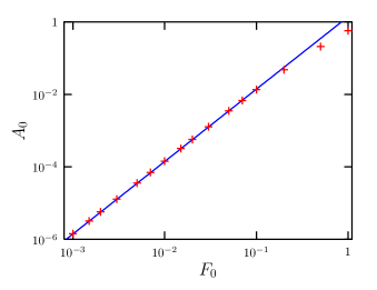
Figure 9: Dependence of the constant term in the Fourier series (59) for $\lambda_{\rm st}(t)$ on the amplitude of the driving force ($+$), in the regime $\epsilon<1$. The parameters are $\gamma=1$, $q=1$, $\epsilon=0.8$ and the frequency is $\omega=\pi/2$. Full line is the function $1.4\,{F_{0}}^{2}$.

Figure 10 exemplifies the evolution of the functions $s_{3}(t)$ and $s_{4}(t)$. We can clearly see that the oscillations are not harmonic. Generally, in the stationary regime these functions are non-harmonic but periodic with the doubled frequency $2\omega$. Thus, the same holds also for the function $\lambda(t)$. Using (56) the stationary response in terms of the switching rate can be written as Fourier series

$$\lambda_{\rm st}(t)=A_{0}+\sum_{k=1}^{\infty}\left(A_{k}\sin 2k\omega t+B_{k}\cos 2k\omega t\right)\quad.$$ (59)

The amplitudes of the harmonic components $A_{0}$, $A_{k},B_{k}$, $k=1,2,...$, satisfy a complicated infinite set of quadratic equations.

To asses the weight of the higher harmonics we performed the fast Fourier transform of the time evolutions obtained by numerical solution, throwing away the initial transient regime. To illustrate the presence of higher harmonics we chose the function $s_{3}(t)$. The modulus of its Fourier transform $\hat{s}_{3}(\nu)=\int s_{3}(t)\,{\rm e}^{-2\pi{\rm i}\,\nu t}\;{\rm d}t$ is shown in Fig. 11. We can clearly see the peaks at the multiples of the basic frequency. We can also observe that the higher harmonics have quite considerable weight. In the inset of Fig. 11 we show also the Fourier transform of the function $\lambda(t)$. Here, the higher harmonics are much less pronounced.

The most important feature of the time evolution under the influence of external harmonic force is the observation that the switching rate remains always positive. This leads to the already mentioned fact that whatever is the coupling strength parameter $\epsilon$, the mean coordinate in stationary regime oscillates around zero, irrespectively of the initial conditions. However, this is the signature of ergodicity, so the glassy behaviour disappears under the influence of arbitrarily small external perturbation. Such a behaviour was already observed also in the model of sheared colloid cates_02 .

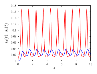
Figure 10: Response of the functions $s_{3}(t)$ (red line) and $s_{4}(t)$ (blue line) to harmonic external driving force for $\gamma=1$, $q=1$, $\epsilon=0.8$, $\omega=\pi$ and $F_{0}=10$.

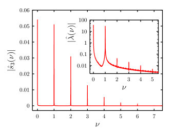
Figure 11: Fourier transform of the stationary oscillations of the function $s_{3}(t)$ under the influence of harmonic external driving force for $\epsilon=0.8$, $\omega=\pi$ and $F_{0}=10$. It was calculated using the fast Fourier transform algorithm. In the inset the Fourier transform of oscillations of the switching rate. The finite width of the peaks, the noise and the continous part of the spectrum in the inset are due to numerical imprecision of the fast Fourier transform procedure.

Both observations can be easily understood. The external force drags the particle back and forth. Once moving, the particle induces through the back-reaction (2) the fluctuations of the environmental force, which prevents the system from freezing in a non-ergodic state. This holds for any positive amplitude of the driving force. However, when the force diminishes, there is still longer transient period, where the system apparently relaxes toward the arrested state, as can be seen qualitatively in Fig. 8. In the limit of infinitesimally small driving, the transient time blows up and the asymptotic state corresponds to the dynamically arrested state. This picture is consistent with the view of glassiness as a purely dynamical phenomenon.

We also observed the response of the system to a signal, which is switched on only after the system relaxed very close to the arrested state. The results can be seen in Fig. 12. Initially, the switching rate relaxes toward zero, but after the perturbation it settles on oscillating behaviour. The average coordinate initially approaches non-zero value (we have chosen initial condition $\langle{\sf Q}_{0}\rangle>0$), but the perturbation brings it to oscillations around zero. This can be interpreted as a schematic picture of shear thinning, although the model is too much simplified to account for the shear thinning quantitatively.

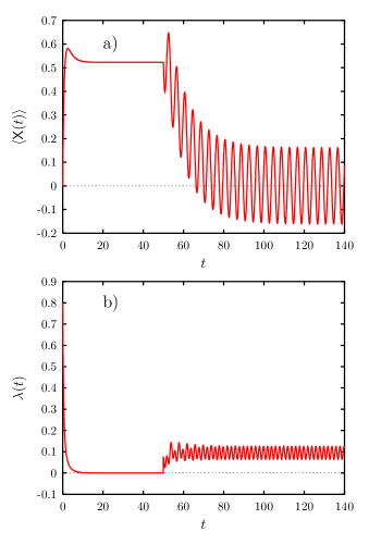
Figure 12: Time evolution of the verage coordinate (a) and switching rate (b) in the regime $\epsilon<1$, when the external harmonic perturbation was switched on at time $t=50$. The parameters are $\gamma=1$, $q=1$, $\epsilon=0.8$, the amplitude of the external perturbation is $F_{0}=0.3$ and the frequency is $\omega=\pi/2$. The initial condition is $\langle{\sf Q}_{0}\rangle=1$.

7 Conclusions

Motivated by the dynamical arrest phenomenon in colloids we formulated and solved a stochastic dynamical model, where the coordinate of a single particle evolves under the influence of stochastic environmental force. The back-reaction couples the switching rate of the force to the average of the square of the velocity of the particle. The strength of the coupling $\epsilon$ is the crucial parameter which determines the behaviour of the system. The problem reduces to a set of coupled non-linear differential equations, which was investigated both analytically and numerically.

The back-reaction induces a phase transition from the ergodic phase for $\epsilon>1$ to the non-ergodic glassy state for $\epsilon<1$. The transition is observed qualitatively in the behaviour of the switching rate, decaying to zero in non-ergodic state, while staying positive in the ergodic state. The Edwards-Anderson parameter, established from the two-time correlation functions, is discontinuous at the transition; it is zero in ergodic phase ($\epsilon>1$), while for $\epsilon<1$ it acquires finite value independent of $\epsilon$. The critical point $\epsilon=1$ is characterised by power-law decay of the switching rate. The leading term $\sim t^{-1}$ in the long-time behaviour was calculated analytically.

We investigated the critical behaviour at $\epsilon\to 1$ through the dependence of the average coordinate in the long-time limit on the initial condition. We find that the asymptotic value of the average coordinate is proportional to the average initial value of the force, where the proportionality factor $\sigma(\epsilon)$ is singular at the transition. In the ergodic phase we have $\sigma(\epsilon)=0$ identically, while in the non-ergodic phase, close to the transition, we found $\sigma(\epsilon)\sim(1-\epsilon)^{1/2}$ for $\epsilon\to 1^{-}$.

Therefore, we find a situation quite unusual from the point of view of static equilibrium phase transition. Indeed, we have two variables, which may be considered as order parameter, namely the Edwards-Anderson parameter and the quantity $\sigma(\epsilon)$. While the former is discontinuous at the critical point, thus indicating first-order transition, the latter is continuous, suggesting second-order transition. the discrepancy is to be attributed to purely dynamical nature of the transition.

Finally, we investigated the response of the system to harmonic external perturbation. We found that the exact response of the coordinate is linear. On the other hand, the response of the variables which are quadratic functions of the coordinate and velocity, like the switching rate, was non-linear and generically contains all higher harmonics, as was seen in the Fourier transform of the signal. We also observed that arbitrarily weak external perturbation is sufficient to “melt” the non-ergodic glassy state and bring it back to ergodic behaviour. We may relate this feature to the notion of stochastic stability parisi_00 ; in this view our system is not stochastically stable. However, our finding is in accord with previously observed behaviour of sheared colloids cates_02 . It makes also connection to the rheological properties of thixotropic fluids vol_nit_hey_reh_02 ; cou_ngu_huy_bon_02 , although our model is too simplified to give quantitative predictions in this direction.

The back-reaction mechanism described by (2) represent the simplest choice. One may ask what would happen if we tried another prescription. We expect that the methods used here will be as well applicable if we generalise (2) as $\lambda(t)=\langle F({\sf V}^{2}(t))\rangle$ for an analytic function $F(x)$. More complicated situation would appear if the dependence was non-local in time, e. g. of the form $\lambda(t)=\int^{t}\langle{\sf V}(t){\sf V}(t^{\prime}))\rangle\,K(t-t^{\prime})\,{\rm d}t^{\prime}$ with some kernel $K(t)$. Such an approach would bring our model closer to the well-studied Mode Coupling equations, but it goes beyond the scope of the present work.

- (1) C. A. Angell, Science 267, 1924 (1995).
- (2) R. G. Palmer, D. L. Stein, E. Abrahams and P. W. Anderson, Phys. Rev. Lett. 53, 958 (1984).
- (3) G. Paladin, M. Mézard and C. de Dominicis, J. Physique Lett. 46, L-985 (1985).
- (4) T. R. Kirkpatrick and D. Thirumalai, Phys. Rev. Lett. 58, 2091 (1987).
- (5) T. R. Kirkpatrick and D. Thirumalai, Phys. Rev. B 36, 5388 (1987).
- (6) T. R. Kirkpatrick, D. Thirumalai and P.G. Wolynes, Phys. Rev. A 40, 1045 (1989).
- (7) F. Ritort, Phys. Rev. Lett 75, 1190 (1995).
- (8) S. Franz and J. Hertz, Phys. Rev. Lett. 74, 2114 (1995).
- (9) L. F. Cugliandolo and J. Kurchan, Phys. Rev. Lett. 71, 173 (1993).
- (10) S. Franz, M. Mézard, G. Parisi, and L. Peliti, Phys. Rev. Lett. 81, 1758 (1998).
- (11) A. Barrat, R. Burioni and M. Mézard, J. Phys. A: Math. Gen. 29, 1311 (1996).
- (12) J. Kurchan, J. Phys. I France 2, 1333 (1992).
- (13) L.F. Cugliandolo and J. Kurchan, Phil. Mag. B 71, 501 (1995).
- (14) E. Marinari, G. Parisi and F. Ritort, J. Phys. A: Math. Gen. 27, 7647 (1994).
- (15) T. M. Nieuwenhuizen, J. Phys. A: Math. Gen. 31, L201 (1998).
- (16) A. Cavagna, I. Giardina, and G. Parisi, Phys. Rev. Lett. 83, 108 (1999).
- (17) A. Cavagna, I. Giardina, and G. Parisi, J. Phys.: Condens. Matter 12, 6295 (2000).
- (18) M. Mézard and G. Parisi, Phys. Rev. Lett. 82, 747 (1999).
- (19) B. Coluzzi, G. Parisi, and P. Verocchio, Phys. Rev. Lett. 84, 306 (2000).
- (20) L.F. Cugliandolo, J. Kurchan, G. Parisi and F. Ritort, Phys. Rev. Lett. 74, 1012 (1995).
- (21) G. Parisi and F. Slanina, Phys. Rev. E 62, 6554 (2000).
- (22) K. Kawasaki and B. Kim, Phys. Rev. Lett. 86, 3582 (2001).
- (23) S. M. Fielding, P. Sollich, and M. E. Cates, J. Rheol. 44, 323 (2000).
- (24) M. Fuchs and M. E. Cates, Faraday Discussions 123, 267 (2003).
- (25) M. E. Cates, preprint cond-mat/0211066.
- (26) A. M. Puertas, M. Fuchs, and M. E. Cates, Phys. Rev. Lett. 88, 098301 (2002).
- (27) M. Fuchs and M. E. Cates, Phys. Rev. Lett. 89, 248304 (2002).
- (28) E. Zaccarelli, G. Foffi, K. A. Dawson, S. V. Buldyrev, F. Sciortino, and P. Tartaglia, Phys. Rev. E 66, 041402 (2002).
- (29) A. Lawlor, D. Reagan, G. D. McCullagh, P. De Gregorio,1 P. Tartaglia, and K. A. Dawson, Phys. Rev. Lett. 89, 245503 (2002).
- (30) E. Stiakakis, D. Vlassopoulos, B. Loppinet, J. Roovers, and G. Meier, Phys. Rev. E 66 , 051804 (2002).
- (31) L. Fabbian, W. Gẗze, F. Sciortino, P. Tartaglia, and F. Thiery , Phys. Rev. E 59, R1347 (1999).
- (32) M. E. Cates, J. P. Wittmer, J.-P. Bouchaud, and P. Claudin, Physica A 263, 354 (1999).
- (33) E. Bertrand, J. Bibette, and V. Schmitt, Phys. Rev. E 66, 060401 (2002).
- (34) W. Götze, in: Liquids, Freezing and Glass Transition, ed. J. P. Hansen, D. Levesque and J. Zinn-Justin, (North-Holland, Amsterdam, 1991) p. 287.
- (35) W. Götze and L. Sjögren, Rep. Prog. Phys. 55, 241 (1992).
- (36) J. P. Bouchaud, L. F. Cugliandolo, J. Kurchan, M. and Mézard, in: Spin glasses and random fields, ed. A. P. Young, (World Scientific, Singapore, 1997) p. 161.
- (37) L. Sjögren, Physica A 322, 81 (2003).
- (38) L. Cugliandolo and J. Kurchan, Physica A 263, 242 (1999).
- (39) P. Chvosta and F. Slanina, J. Phys. A: Math. Gen. 35, L277 (2002).
- (40) W. Horsthemke and R. Lefever Noise-Induced Transitions. Theory and Applications in Physics, Chemistry and Biology Springer Series in Synergetics, vol. 15, (Springer, Berlin, 1984).
- (41) D. R. Cox Renewal Theory (Wiley, New York, 1962).
- (42) D. L. Snyder Random Point Processes (Wiley, New York, 1975).
- (43) Y. Pomeau J. Stat. Phys. 24, 189 (1981).
- (44) P. Sibani and N. G. van Kampen Physica A 122, 397 (1983).
- (45) A. Morita Phys. Rev. A 41, 754 (1990).
- (46) M. Abramowitz and I. A. Stegun (editors) Handbook of Mathematical Functions (Dover, New York, 1970).
- (47) G. Parisi, preprint cond-mat/0007347.
- (48) C. Völtz, M. Nitschke, L. Heymann, and I. Rehberg, Phys. Rev. E 65, 051402 (2002).
- (49) P. Coussot, Q. D. Nguyen, H. T. Huynh, and D. Bonn, Phys. Rev. Lett. 88, 175501 (2002).