Cycles structure and local ordering in complex networks

Abstract

We study the properties of metrics aimed at the characterization of grid-like ordering in complex networks. These metrics are based on the global and local behavior of cycles of order four, which are the minimal structures able to identify rectangular clustering. The analysis of data from real networks reveals the ubiquitous presence of a high level of grid-like ordering that is non-trivially correlated with the local degree properties. These observations provide new insights on the hierarchical structure of complex networks.

Many networks arising in social, biological, and technological contexts are growing and self-organizing systems which are not modeled by any supervising entity, nor follow an externally defined blueprint [1, 2, 3, 4, 5]. Empirical evidences, indeed, have prompted that most of the times the network’s topology exhibits complex features which cannot be explained by merely extrapolating the local properties of their constituents. The most relevant among these features are the small-world property [6, 3] and a high level of heterogeneity, usually reflected in a scale-free behavior of the network’s connectivity [7]. While these properties would prompt to a very large degree of randomness, yet real networks exhibit a surprising level of structural ordering. This fact has been first pointed out by noting the common property of many networks to form cliques in which every element is linked to every other element; i.e. the presence of a high clustering coefficient [6], defined as the fraction of triangles present in the network. The identification of hidden ordering and hierarchies in the seemingly haphazard appearance of real networks is therefore a major area of study, aimed at understanding their basic organizing principles. This activity has led to a harvest of results concerning nontrivial correlation properties among the various elements of natural networks, suggesting the presence of interesting modular organizations [8, 9, 10, 11].

In this paper we point out that the usual clustering coefficient is in some cases unable to quantify the order underlying a network’s structure. In particular, a general modular structure is represented by a grid-like frame, such as a regular hypercubic lattice, that can be adequately quantified only by evaluating the frequency of rectangular loops appearing in the network. We introduce a grid coefficient that allows us to uncover the presence of a surprising level of grid ordering in several real networks ranging from technological (the physical Internet) to social (scientific collaboration network) systems. By correlating the presence of grid-like structures with the local connectivity properties we are able to uncover the presence of a scaling hierarchy that appears to be a widely present organizing principle. In some cases, the scaling behavior of the grid clustering is very similar to the triangle clustering, suggesting a kind of statistical self-similarity in the modular construction of the network.

A network (or graph in the mathematical language [12]) is a set of vertices and edges joining pairs of vertices, representing individuals and the interactions among them, respectively. Two features play a special role in the characterization of complex networks. The first one refers to the small-world concept [6]: i.e. the small average distance in terms of number of edges between any two vertices in the system. The second consists in a very high heterogeneity, usually reflected in a scale-free distribution $P(k)\sim k^{-\gamma}$ for the probability that any given vertex has degree $k$; i.e. $k$ edges to other vertices [7]. Both properties appear as ubiquitous in dynamically growing networks [1, 2]. Real networks also show a large degree of local clustering and correlations. A first quantitative measurements of these properties is provided by the clustering coefficient [6] and the average nearest neighbors degree [8, 10]. In particular, the clustering coefficient $c_{i}$ of the vertex $i$, with degree $k_{i}$, is defined as the ratio between the number of edges $e_{i}$ in the sub-graph identified by its nearest neighbors and its maximum possible value, $k_{i}(k_{i}-1)/2$, corresponding to a complete sub-graph, i.e. $c_{i}=2e_{i}/k_{i}(k_{i}-1)$. The average clustering coefficient $\langle c\rangle$ is defined as the average value of $c_{i}$ over all the vertices in the graph, $\langle c\rangle=\sum_{i}c_{i}/N$, where $N$ is the size (total number of vertices) of the network. This magnitude quantifies the tendency that two vertices connected to the same vertex are also connected to each other; therefore it measures the ordering in the system. By comparison, random graphs [13] are not clustered, having $\langle c\rangle=\langle k\rangle/N$, where $\langle k\rangle$ is the average degree, while regular lattices tend to be highly clustered with their neighbors. Further information can be extracted if one computes the average clustering coefficient $c(k)$ as a function of the vertex degree $k$ [9].

In the physics terminology, the study of the clustering coefficient $c(k)$ is strictly related to the analysis of three-point correlation functions [14]. The absolute average value—as well as the scaling with $k$—of this quantity are fundamental to discriminate the level of randomness and the organizing principles related to the basic hierarchies present in the networks. For instance, a large class of scale-free networks shows a clustering coefficient decaying as a power-law as a function of the vertex’s degree [11]. This implies that low degree vertices tend to form connected cliques with other vertices, while large connected vertices (hubs) tend to act as bridges between unconnected cliques, thus showing a small clustering coefficient. This fact highlights the existence of some modular building, identified by the cliques of small degree vertices [11].

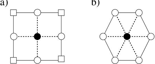
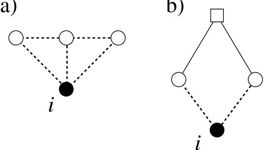
With the aim of unveiling the hidden ordering in complex networks the use of the two- and three-point correlations is however not always sufficient. As a very simple example we can consider a rectangular lattice or grid, Fig. 1(a). In this case it easy to recognize that the clustering coefficient is not able to distinguish any ordering in a grid-like structure, since its value is always null. However, it is a good measure of order for other regular structures, such as a triangular lattice, Fig. 1(b). Since grid-like structures are among the preferred ordered patterns in natural systems, we introduce as a further quantitative characterization of networks’ regularity some metrics that naturally account for rectangular symmetries [15, 16, 17]. We start by considering the closed paths in a network in which all edges and vertices are distinct. These closed paths are known as cycles [12]. Cycles of length $3$ (i.e. composed by three vertices) are called triangles. The ratio between the number of triangles that include the vertex $i$, $e_{i}$, and its maximum possible number, $k_{i}(k_{i}-1)/2$, defines the triangle coefficient of the vertex $i$, which is by definition equal to its clustering coefficient $c_{i}$. Cycles of length $4$ are called quadrilaterals. In the spirit of the clustering coefficient, we want to improve the measurement of the network structure by using the grid coefficient, $c_{4,i}$, that is defined as the fraction of all the quadrilaterals passing by the vertex $i$, $Q_{i}$, divided by the maximum possible number of quadrilaterals sharing the vertex $i$, $Z_{i}$. Interestingly, the grid coefficient can be further decomposed by noting that each quadrilateral passing by $i$ is composed by the vertex $i$ itself plus three external vertices. Quadrilaterals can be therefore classified according to the nature of the external vertices, see Fig. 2. If all the external vertices are nearest neighbors of $i$, they form a primary quadrilateral; on the other hand, if one of the external vertices is a second neighbor of $i$, the cycle they form is a secondary quadrilateral. If the vertex $i$ has degree $k_{i}$ and it is connected to $k^{nn}_{i}$ second neighbors, it is easy to check that the maximum number of primary quadrilaterals is $Z_{i}^{p}=3\times\binom{k_{i}}{3}=k_{i}(k_{i}-1)(k_{i}-2)/2$, while the maximum number of secondary quadrilaterals is $Z_{i}^{s}=k^{nn}_{i}k_{i}(k_{i}-1)/2$. In this way, in order to study the grid properties of a network, we can define three magnitudes: the primary grid coefficient, $c_{4,i}^{p}=Q_{i}^{p}/Z_{i}^{p}$, the secondary grid coefficient $c_{4,i}^{s}=Q_{i}^{s}/Z_{i}^{s}$, and the total grid coefficient $c_{4,i}=(Q_{i}^{p}+Q_{i}^{s})/(Z_{i}^{p}+Z_{i}^{s})$, where $Q_{i}^{p}$ and $Q_{i}^{s}$ are the actual number of primary and secondary quadrilaterals passing by the node $i$, respectively. The respective average grid coefficients are defined by averaging these quantities over all vertices in the network.

As an example of this definition, let us consider the rectangular lattice represented in Fig. 1(a), in which each vertex $i$ has $4$ nearest neighbors and $8$ second neighbors. There are no primary quadrilaterals passing by any node $i$, while the number of secondary quadrilaterals is $Q^{s}=4$. From here we obtain $\langle c^{p}_{4}\rangle=0$, $\langle c^{s}_{4}\rangle=1/9$, and $\langle c_{4}\rangle=1/15$. On the other hand, in the triangular lattice, Fig. 1(b), in which each vertex has $6$ nearest neighbors and $12$ second neighbors, we find $6$ primary quadrilaterals and $6$ secondary quadrilaterals, which yield $\langle c^{p}_{4}\rangle=1/10$, $\langle c^{s}_{4}\rangle=1/30$, and $\langle c_{4}\rangle=1/20$. Thus, regular grids exhibit a finite grid coefficient, in opposition to the clustering coefficient, which is zero for any hypercubic lattice.

A very different case is represented by the Erdös-Rényi random graph [13, 18, 19], constructed from a set on $N$ vertices that are joined in pairs by an edge with probability $p$. In this case the emerging network has average degree $\langle k\rangle=pN$ and a Poisson degree distribution, and it is completely random, so that any ordering is absent in the infinite size limit. It is possible to calculate easily the grid coefficients for this network. For any vertex $i$, we need at least three nearest neighbors to construct a primary quadrilateral. Given this configuration, the probability to close the cycle in any of the three possible quadrilaterals is given by the probability $p^{2}$ to draw two edges between two of the three nearest neighbors. Therefore we have that for any vertex $c^{p}_{4,i}=p^{2}$. This implies that an Erdös-Rényi random graph of $N$ vertices and given average connectivity $\langle k\rangle$ has an average primary grid coefficient $\langle c^{p}_{4}\rangle=\left(\langle k\rangle/N\right)^{2}\sim N^{-2}$. The calculation for the secondary grid coefficient is slightly more involved. In this case, for any vertex $i$, we need at least two nearest neighbors and a second neighbor. This last vertex, being a second neighbor, is connected to at least one nearest neighbor, but not necessarily to any of the two nearest neighbors that will compose the quadrilateral. If the second neighbor is not a priori connected to the two nearest neighbors, then the probability of finding a quadrilateral is of order $p^{2}$. On the other hand, if it is a priori connected to one of the selected nearest neighbors, the probability of closing a quadrilateral is just $p$; i.e. the probability of drawing an edge between the second neighbor and the remaining nearest neighbor. This last instance (that the second neighbors is a priori connected to one of the nearest neighbors considered) happens with probability $1/k_{i}$, where $k_{i}$ is the degree of the vertex $i$. Therefore, at leading order in $p$, we have that for any vertex $c^{s}_{4,i}=p/k_{i}$. The average secondary grid coefficient is then given by $\langle c^{s}_{4}\rangle=\sum_{k\geq 2}P(k)p/k\equiv\left<1/k\right>^{\prime}\langle k\rangle/N$, where $P(k)$ is the degree distribution of the Erdös-Rényi random graph [19]. By summing both contributions we have that at leading order, the average total grid coefficient is scaling as $\langle c_{4}\rangle\sim p$. In general thus the grid coefficient for random graphs of given average connectivity scales as $\langle c_{4}\rangle\sim N^{-1}$ with the number of vertices $N$.

In order to characterize the level of grid-like ordering in real networks, we have measured the grid coefficients in four different systems, characterized by a scale-free degree distribution, which have been the focus of several recent studies:

Internet: Internet map at the Autonomous System (AS) level, as of 22nd November 1999 [8, 9, 20]. These maps are collected and made publicly available by the National Laboratory for Applied Network Research. Each AS refers to one single administrative domain of the Internet. Different ASs are in most cases connected through a Border Gateway Protocol (BGP) that identifies any AS through a $16$-bit number. The map considered is composed by $6243$ ASs acting as vertices and by $12113$ BGP peer connections, acting as edges, yielding an average degree $\langle k\rangle=3.88$.

World-Wide-Web: Map of the World-Wide-Web collected at the domain of Notre Dame University [21, 22, 23]. This network is actually directed, but we have considered it as non-directed. The map is composed by $325729$ web pages, represented by vertices, and $1090108$ hyperlinks pointing from one page to another, represented by edges, which corresponds to an average degree $\langle k\rangle=6.69$.

Movie actor collaborations: Network of co-actorship obtained from the Internet Movie Database [6, 7, 24, 25]. In this case the $82583$ actors represent the vertices of the graph. An edge is drawn between two actors if they have played together in at least one movie. The total number of edges is $3666738$, with an average degree $\langle k\rangle=88.80$.

Scientific collaborations: Network of scientific collaborations collected from the condensed matter preprint database at Los Alamos [26, 27, 28]. This web site hosts the largest collection of preprints in condensed matter physics. The graph is composed by $16264$ different authors, that are connected by one edge if they have coauthored a joint paper. The total amount of collaborations (edges) is then $47594$, yielding an average degree $\langle k\rangle=5.85$. One can assign a weight to such links, by counting how many joint paper are present in the repositories. In this first approach we only considered the topological connections given by the unweighted links.

In Table 1 we report the different average grid coefficients for all the networks analyzed, compared with those corresponding to the Erdös-Rényi random graph, the rectangular grid and the triangular lattice. It is interesting to note that the average grid coefficients of all networks are two to four orders of magnitude larger than the corresponding coefficients of a random graph with the same average degree and size $N$. While the small-world property and the scale-free degree distribution common to all these networks are generally associated to randomness and large fluctuations, the presence of large grid coefficient makes those graphs reminiscent of a grid-like ordering, very probably due to the presence of hierarchical structures and well-defined communities.

More information can be gathered by studying the grid coefficient as a function of the vertex’s degree $k$ (i.e. by considering the average value $c_{4}(k)$ of the total grid coefficient for all the vertices with the same degree $k$). As similarly noticed for the clustering coefficient [9, 11], the grid coefficient is well approximated in most cases by a power-law decay for increasing $k$. This feature indicates a correlation between the vertices’ degree and the local network structure. In particular, low degree vertices are arranged in fairly ordered patterns whose building blocks are triangular and rectangular structures. Vertices with large degree act as the network backbone by connecting the highly clustered regions. Since we are facing power-law behavior for the clustering and grid coefficient, we have that no characteristic length scales are present in the system and thus there is a continuum hierarchy of structures. It is also worth remarking that the grid coefficient is always smaller than the clustering coefficient because it represents a measure of longer range correlations. Even though statistical fluctuations are comparable, in some cases the grid coefficient appears to be less susceptible to noise than other metrics. Finally, we note the presence of two classes of networks: the first with a scaling of the $c_{4}(k)$ very similar to $c(k)$ (such as the technological Internet and World-Wide-Web networks), and a second one with $c_{4}(k)$ different from $c(k)$ (as is the case of the social networks). When the power-law behavior is alike, we can talk of self-similar networks in which both rectangular and triangular patterns are equally implemented in the modular construction of the network. In the second situation, one of the two patterns is abandoned earlier in the hierarchical construction of the graph, breaking the self-similarity at all levels of the hierarchy.

Figure 1: (a) Regular square lattice. Nearest neighbors of a vertex (empty circles) are not neighbors of each other. Therefore the clustering coefficient $c_{i}\equiv 0$ for every vertex $i$. (b) Triangular lattice. Here some of the neighbors are connected to each other. In particular $2$ out of every $5$ possible edges are drawn; hence $c_{i}=2/5$ for all the vertices

Figure 2: (a) Example of a primary quadrilateral, in which the three external vertices are nearest neighbors of the vertex $i$. (b) Example of a secondary quadrilateral in which one of the external vertices (empty square) is a second neighbor of the vertex $i$ .

   

   

Figure 3: Clustering coefficient $c(k)$ (hollow symbols) and grid coefficient $c_{4}(k)$ (filled symbols) as a function of the node degree, for the networks considered. (a) Internet at the AS level. (b) Map of the World-Wide-Web domain collected at www.nd.edu. (c) Network of co-actorship from the Internet Movie Database. (d) Scientific collaborations from the cond-mat preprint database.

	$\langle k\rangle$	$\langle c\rangle$	$\langle c^{p}_{4}\rangle$	$\langle c^{s}_{4}\rangle$	$\langle c_{4}\rangle$
Internet	$3.88$	$0.25$	$0.043$	$0.028$	$0.028$
World-Wide-Web	$6.69$	$0.23$	$0.14$	$0.088$	$0.090$
movie actor collaborations	$88.80$	$0.75$	$0.66$	$0.009$	$0.027$
scientific coauthorship	$5.85$	$0.64$	$0.40$	$0.036$	$0.12$
Erdös-Rényi random graph	$Np$	$\sim N^{-1}$	$\sim N^{-2}$	$\sim N^{-1}$	$\sim N^{-1}$
square lattice	$4$	$0$	$0$	$1/12$	$1/15$
triangular lattice	$6$	$2/5$	$1/10$	$1/30$	$1/20$

Table 1: Average degree, clustering coefficient, and primary, secondary, and total grid coefficients for the different networks considered (see text).

References

- [1] Albert, R & Barabási, A.-L. (2002) Rev. Mod. Phys. 74, 47–97.
- [2] Dorogovtsev, S. N & Mendes, J. F. F. (2002) Adv. Phys. 51, 1079–1187.
- [3] Watts, D. J. (1999) Small worlds: the dynamics of networks between order and randomness. (Princeton University Press, New Jersey).
- [4] Barabási, A. L. (2002) Linked; The new science of networks. (Perseus Publishing, Cambridge).
- [5] Buchanan, M. (2002) Small World: Uncovering Nature’s hidden networks. (Weidenfeld & Micolson, London).
- [6] Watts, D. J & Strogatz, S. H. (1998) Nature 393, 440–442.
- [7] Barabási, A.-L & Albert, R. (1999) Science 286, 509–511.
- [8] Pastor-Satorras, R, Vázquez, A, & Vespignani, A. (2001) Phys. Rev. Lett. 87, 258701.
- [9] Vázquez, A, Pastor-Satorras, R, & Vespignani, A. (2002) Phys. Rev. E 65, 066130.
- [10] Newman, M. E. J. (2002) Phys. Rev. Lett. 89, 208701.
- [11] Ravasz, E & Barabási, A.-L. (2002) Hierarchical organization in complex networks. e-print cond-mat/0206130.
- [12] Bollobás, B. (1998) Modern Graph Theory. (Springer-Verlag, New York).
- [13] Erdös, P & Rényi, P. (1959) Publicationes Mathematicae 6, 290–297.
- [14] Vázquez, A, Pastor-Satorras, R, & Vespignani, A. (2002) Internet topology at the router and autonomous system level. cond-mat/0206084.
- [15] Vázquez, A, Flammini, A, Maritan, A, & Vespignani, A. (2001) Modelling of protein interaction networks. cond-mat/0108043.
- [16] Holme, P, Edling, C. R, & Liljeros, F. (2002) Structure and time-evolution of the Internet community pussokram.com. e-print cond-mat/0210514.
- [17] Bianconi, G & Capocci, A. (2002). (Private communication).
- [18] Bollobás, B. (1985) Random graphs. (Academic Press, London).
- [19] Newman, M. E. J. (2002) in Handbook of Graphs and Networks: From the Genome to the Internet, eds. Bornholdt, S & Schuster, H. G. (Wiley-VCH, Berlin).
- [20] Faloutsos, M, Faloutsos, P, & Faloutsos, C. (1999) Comput. Commun. Rev. 29, 251–263.
- [21] Albert, R, Jeong, H, & Barabási, A.-L. (1999) Nature 401, 130–131.
- [22] Barabási, A.-L, Albert, R, & Jeong, H. (2000) Physica A 281, 69–77.
- [23] Huberman, B. A & Adamic, L. A. (1999) Nature 401, 131.
- [24] Newman, M. E. J, Strogatz, S. H, & Watts, D. J. (2001) Phys. Rev. E 64, 026118.
- [25] Amaral, L. A. N, Scala, A, Barthélémy, M, & Stanley, H. E. (2000) Proc. Natl. Acad. Sci. USA 97, 11149–11152.
- [26] Newman, M. E. J. (2001) Phys. Rev. E 64, 016131.
- [27] Newman, M. E. J. (2001) Phys. Rev. E 64, 016132.
- [28] Barabási, A.-L, Jeong, H, Ravasz, R, Néda, Z, Vicsek, T, & Schubert, A. (2002) Physica A 311, 590–614.