Multiparticle Landau-Zener problem.

Abstract

We propose a simple ansatz that allows to generate new exactly solvable multi-state Landau-Zener models. It is based on a system of two decoupled two-level atoms whose levels vary with time and cross at some moments. Then we consider multiparticle systems with Heisenberg equations for annihilation operators having similar structure with Shrödinger equation for amplitudes in multistate Landau-Zener models and show that the corresponding Shrödinger equation in multiparticle sector belongs to the multistate Landau-Zener class. This observation allows to generate new exactly solvable models from already known ones. We discuss possible applications of the new solutions in the problem of the driven charge transport in quantum dots.

I Introduction.

Landau-Zener (LZ) theory [1, 2] is one of the most important and influential results in non-stationary quantum mechanics. Last decade a generalization of LZ theory to more than two states attracted particular attention due to numerous applications in atomic and molecular physics [3], [4], nanomagnets [5], Bose-Einstein condensate [6] and systems with avoided band crossings [7], [8]. The multi-state LZ problem (see for example [9] ) is concerned with finding of the transition amplitudes for a system with the Hamiltonian, whose matrix form reads:

$$H=Bt+A,$$ (1)

where $B$ is a diagonal matrix and the matrices $A$ and $B$ are independent of time. In its general form this problem is still unsolved, but a number of exact results for special choices of the matrices $B$ and $A$ were found [9, 10, 11, 12, 13, 14, 15, 16, 17, 18, 19].

In almost all available exact solutions the transition probabilities are expressed in terms of the genuine two-level LZ formula successively applied at each diabatic level intersection. In other physical problems such a procedure is often applied as an approximation. These problems include atomic and molecular collisions [20] and the transitions at crossing of two Rydberg multiplets of energy levels [3].

In this work we find very simple ansatz that generates new solvable models and may explain the properties of already known solutions. The main idea employs the single-particle Hamiltonian which acts independently in several two-dimensional subspaces of the Hilbert space. It is worth mentioning that while results in one-particle sector are trivial, the same Hamiltonian generates non-trivial solutions in the many particle spaces. Such a construction is akin to the group-theoretical method of finding higher irreducible representations as a symetrized direct product of the fundamental representation. Using this method we can study the problem of driven charge transport through a quantum dot and find new solutions in multistate LZ theory. Particularly, we derive the transition probabilities for a four state LZ problem which is very similar to the four state bow-tie model and for a problem of intersection of two bands of parallel levels.

This article is organized as follows: in section II we show how already known solutions of LZ models can generate new exactly solvable models with the Hamiltonian (1). We demonstrate how the exact solution for two independent two level systems can generate a new solution of a four-state LZ model. In III we generalize Demkov-Osherov solution to the case of many particles and use the result for derivation of master equations that describe a driven charge transport in quantum dots. In IV we provide an example of a solvable model that can be generated from the Demkov-Osherov solution.

II Bosonic multi-state LZ models.

Lets consider a Hamiltonian that describes the interaction of four bosonic fields $\hat{a},\,\hat{b},\,\hat{c},\,\hat{d}$:

$$\begin{array}[]{l}\hat{H}=(\beta_{1}t+E_{1})\hat{a}^{+}\hat{a}+(\beta_{3}t+E_{3})\hat{d}^{+}\hat{d}+(\beta_{2}t+E_{2})\hat{c}^{+}\hat{c}+(\beta_{4}t+E_{4})\hat{b}^{+}\hat{b}+\\ g(\hat{a}^{+}\hat{b}+\hat{b}^{+}\hat{a})+\gamma(\hat{c}^{+}\hat{d}+\hat{d}^{+}\hat{c})\end{array}$$ (2)

This Hamiltonian depends explicitly on time and conserves the total number of particles in the system. Therefore it can be considered independently in subspaces with fixed total number of particles. Let $|0>$ be the vacuum state. The Hamiltonian (2) describes the evolution of two disjointed systems. However, being projected onto the 2-particle sector, its matrix form looks less trivial. The complete two-particle sector is the 10-dimensional Hilbert space spanned onto direct products of any two single-particle states. The four-dimensional subspace $R_{4}$ of the 2-particle sector spanned onto vectors:

$$\begin{array}[]{l}|1>=\hat{a}^{+}\hat{c}^{+}|0>\\ |2>=\hat{a}^{+}\hat{d}^{+}|0>\\ |3>=\hat{d}^{+}\hat{b}^{+}|0>\\ |4>=\hat{c}^{+}\hat{b}^{+}|0>\end{array}$$ (3)

is invariant with respect to the action of the Hamiltonian (2). Hence, if the initial state belongs to this subspace, the state vector at any time remains in $R_{4}$:

$$|\psi(t)\rangle=c_{1}(t)|1\rangle+c_{2}(t)|2\rangle+c_{3}(t)|3\rangle+c_{4}(t)|4\rangle$$ (4)

In the basis (3) the Hamiltonian (2) has the following 4x4 matrix form:

$$H=\left(\begin{array}[]{llll}(\beta_{1}+\beta_{2})t+(E_{1}+E_{2})&\,\,\gamma&0&g\\ \gamma&(\beta_{1}+\beta_{3})t+(E_{1}+E_{3})&g&0\\ 0&g&(\beta_{3}+\beta_{4})t+(E_{3}+E_{4})&\gamma\\ g&0&\gamma&(\beta_{2}+\beta_{4})t+(E_{4}+E_{2})\end{array}\right)$$ (5)

The problem described by the Hamiltonian (5) belongs to the multistate Landau-Zener class (1).

We should point out that it cannot be mapped on the already known exactly solvable multistate LZ models.

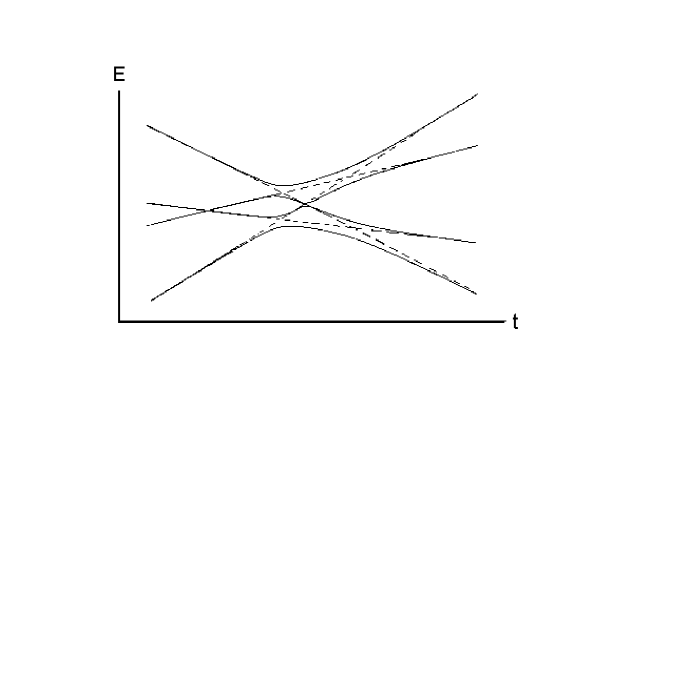
FIG. 1.: Time dependence of the adiabatic energies (solid lines) and diagonal elements (dashed lines) of the Hamiltonian (5). The choice of parameters is $\beta_{1}=5,\,\beta_{2}=-3,\,\beta_{3}=0,\,\beta_{4}=-1.5,\,E_{1}=3,\,E_{2}=0.5,\,E_{3}=-2,\,E_{4}=-1.5,\,g=1,\,\gamma=1.5$

In $Fig.1$ we show the adiabatic energies of the Hamiltonian (5) as functions of time for typical choice of parameters. It is clearly seen that there is a point of an exact adiabatic level crossing (diabolic point) on the figure.

In the Heisenberg representation the evolution equations decouple into two pairs of equations for bosonic operators:

$$\begin{array}[]{l}i\dot{\hat{a}}=(\beta_{1}t+E_{1})\hat{a}+g\hat{b}\\ i\dot{\hat{b}}=(\beta_{4}t+E_{4})\hat{b}+g\hat{a}\end{array}$$ (6)

and

$$\begin{array}[]{l}i\dot{\hat{c}}=(\beta_{2}t+E_{2})\hat{c}+\gamma\hat{d}\\ i\dot{\hat{d}}=(\beta_{3}t+E_{3})\hat{d}+\gamma\hat{c}\end{array}$$ (7)

Let $\hat{a}_{0},\hat{b}_{0},\hat{c}_{0},\hat{d}_{0}$ denote the operators $\hat{a},\hat{b},\hat{c},\hat{d}$ at the initial moment of evolution. Then the solutions of equations (6) and (7) are:

$$\begin{array}[]{l}\hat{a}(t)=S_{11}(t)\hat{a}_{0}+S_{12}(t)\hat{b}_{0}\\ \hat{b}(t)=S_{21}(t)\hat{a}_{0}+S_{22}(t)\hat{b}_{0}\end{array}$$ (8)

$$\begin{array}[]{l}\hat{c}(t)=S_{11}^{\prime}(t)\hat{c}_{0}+S_{12}^{\prime}(t)\hat{d}_{0}\\ \hat{d}(t)=S_{21}^{\prime}(t)\hat{c}_{0}+S_{22}^{\prime}(t)\hat{d}_{0}\end{array}$$ (9)

Here $S_{ij}$ and $S_{ij}^{\prime}$ are the matrix elements of the evolution operators for (6) and (7), respectively. Due to the linearity they are the same for the operator and numerical functions obeying these differential equations. Hence, we can extract them directly from the solution of the two-state LZ problem. For the evolution from $t=-\infty$ to $t=+\infty$ their squares of modulus are:

$$\begin{array}[]{l}p_{1}\equiv|S_{11}|^{2}=|S_{22}|^{2}=e^{-2\pi g^{2}/|\beta_{1}-\beta_{4}|}\\ q_{1}\equiv|S_{12}|^{2}=|S_{21}|^{2}=1-p_{1}\\ p_{2}\equiv|S_{11}^{\prime}|^{2}=|S_{22}^{\prime}|^{2}=e^{-2\pi\gamma^{2}/|\beta_{2}-\beta_{3}|}\\ q_{2}\equiv|S_{12}^{\prime}|^{2}=|S_{21}^{\prime}|^{2}=1-p_{2}\\ \end{array}$$ (10)

Returning to the four-state LZ problem in the two-particle sector considered earlier, we first note that each state $|\gamma\rangle$ of this subspace is the direct product of states from two independent subspaces of the one-particle sector $|j\rangle=|\alpha_{j}\rangle\bigotimes|\mu_{j}\rangle$, $\alpha_{j}=1,2;\mu_{j}=3,4$ (note that here 1,2,3,4 enumerate single-particle state, for example $|1\rangle=a^{+}|0\rangle$). The evolution matrix is also the direct product of evolution matrices in the independent subspaces of the one-particle sectors: $U(t)=U_{\alpha}(t)\bigotimes U_{\mu}(t)$. Therefore transition matrix elements and probabilities $P_{ij}$ in the considered subspace are factorized:

$$P_{ij}=p_{\alpha_{i}\alpha_{j}}p_{\mu_{i}\mu_{j}}$$ (11)

In terms of the LZ probabilities for two-level problems introduced earlier the transition probability matrix $P$, whose elements are defined by equation (11), reads:

$$P=\left(\begin{array}[]{llll}p_{1}p_{2}&p_{1}q_{2}&q_{1}q_{2}&p_{1}q_{2}\\ p_{1}q_{2}&p_{1}p_{2}&q_{1}p_{2}&q_{1}q_{2}\\ q_{1}q_{2}&p_{2}q_{1}&p_{1}p_{2}&p_{1}q_{2}\\ q_{1}p_{2}&q_{1}q_{2}&p_{1}q_{2}&p_{1}p_{2}\end{array}\right)$$ (12)

This result does not depend on the parameters $E_{i}$. It is interesting that scattering matrices $S_{ij}(t)$ and $S_{ij}^{\prime}(t)$ are known for any $t$ [2] which make it possible to find the evolution operator at any time in the Schrödinger representation.

III Driven charge transport through quantum dots.

In similar fashion to the previous section the fermionic systems can lead to Heisenberg equations for annihilation operators that have the same structure as Shrödinger equation for amplitudes for some exactly solvable multistate Landau-Zener model. As we will show, in the Shrödinger representation such a Fermi system with fixed number of particle is equivalent to a new solvable multistate Landau-Zener model. The models that we will examine correspond to the driven charge transport in nanostructures.

Consider a quantum dot coupled to an external reservoir like the system shown in $Fig2$. Lets consider that initially some of the reservoir energy levels are filled with electrons, the others are empty. Lets assume the dot has only one electron bound state whose energy in real semiconductors can be regulated by the gate voltage; therefore the variation of the gate voltage with time generates time dependence of the dot’s electronic level.

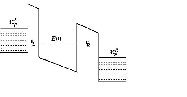
FIG. 2.: A single energy level in a potential well coupled to two leads at zero temperature. Electron states in leads are filled up to Fermi energies, that can be different in right and left leads.

The Hamiltonian of the electrons in the dot and reservoir reads:

$$H=\sum\limits_{n=1}^{N}E_{n}\hat{c}_{n}^{+}\hat{c}_{n}+E(t)\hat{c}_{0}^{+}\hat{c}_{0}+\sum\limits_{n}g_{n}(\hat{c}_{n}^{+}\hat{c}_{0}+\hat{c}_{0}^{+}\hat{c}_{n})$$ (13)

Here $\hat{c_{0}}$ is the fermionic operator that annihilates the electron on the dot level and $\hat{c}_{n}$ is the annihilation operators for the level $E_{n}$ of the reservoir; $E(t)$ is the time-dependent energy of the dot state. In our treatment the last term in (13) describes the tunneling between the leads and the single level in the quantum dot. We ignore all interactions among electrons except the one due to Pauli principle.

Similar time-dependent single-particle problems for quantum dots have been already considered in [21]. Though our system is simplified but rather it is interesting because it has an exact solution.

In the context of LZ theory, we approximate the dot energy by a linear function of time: $E(t)=\beta t$. The Heisenberg operator equations corresponding to Hamiltonian (13) are:

$$\begin{array}[]{l}i\dot{\hat{c}}_{0}=\beta t\hat{c}_{0}+\sum\limits_{n}g_{n}\hat{c}_{n}\\ i\dot{\hat{c}}_{n}=E_{n}\hat{c}_{n}+g_{n}\hat{c}_{0}\end{array}$$ (14)

Due to the linear structure of these equations the solution can be formally written in the matrix form:

$$\vec{\hat{c}}(t)=\hat{S}(t)\vec{\hat{c}}(t_{0})$$ (15)

where $\vec{\hat{c}}=(\hat{c}_{0},\hat{c}_{1},\ldots,\hat{c}_{n})$

As in the previous section, the evolution matrix $\hat{S}(t)$ is completely determined by the coefficients of the differential equations (14) and is the same for operator and c-function solutions. Hence, it is enough to solve (14) with all operators replaced by c-functions. Such a system of equations coincides with that of the Demkov-Osherov model [18]. The latter provides transition amplitudes for a single energy level crossing an energy band consisting of time-independent levels.

In Demkov-Osherov model the Shrödinger equation for the amplitudes of different quantum states can be written as follows:

$$i\left({\begin{array}[]{*{20}c}{\dot{a}_{0}(t)}\\ {\dot{a}_{1}(t)}\\ \vdots\\ {\dot{a}_{n}(t)}\\ \end{array}}\right)=\left({\begin{array}[]{*{20}c}{\beta t}&{\gamma_{1}}&\cdots&{\gamma_{n}}\\ {\gamma_{1}^{*}}&{\alpha_{1}}&\cdots&0\\ \vdots&\vdots&\ddots&\vdots\\ {\gamma_{n}^{*}}&0&\cdots&{\alpha_{n}}\\ \end{array}}\right)\left({\begin{array}[]{*{20}c}{a_{0}(t)}\\ {a_{1}(t)}\\ \vdots\\ {a_{n}(t)}\\ \end{array}}\right)$$ (16)

where $\alpha_{k}$ are ordered as follows $\alpha_{1}<\alpha_{2}<...<\alpha_{N_{a}}$ (assuming that none two of the $\alpha_{k}$ are equal; we also assume for definiteness that $\beta>0$).

The absolute values of the $S$-matrix components ($S_{kl}=|a_{k}^{(l)}(\infty)|/a_{l}^{(l)}(-\infty)|)$ [18] are:

$$\begin{array}[]{l}S_{00}=e^{-\pi(z_{1}+\ldots+z_{n})}\\ S_{0l}=(1-e^{-2\pi z_{l}})^{1/2}e^{-\pi(z_{l+1}+\ldots+z_{n})}\\ S_{k0}=e^{-\pi(z_{1}+\ldots+z_{k-1})}(1-e^{-2\pi z_{k}})^{1/2},(k=1,\ldots,n)\\ S_{kl}=0,(1\leq k<l)\\ S_{ll}=e^{-\pi z_{l}}\\ S_{kl}=(1-e^{-2\pi z_{l}})^{1/2}e^{-\pi(z_{l+1}+\ldots+z_{k-1})}(1-e^{-2\pi z_{k}})^{1/2},(k>l)\end{array}$$ (17)

(where the index $l=1\ldots n$ and $z_{k}=|\gamma_{k}|^{2}/\beta$)

The probabilities to find an electron on a particular $n$-th level are.

$$\begin{array}[]{l}P_{n}=<\hat{c}_{n}^{+}(t\rightarrow+\infty)\hat{c}_{n}(t\rightarrow+\infty)>=\sum_{n_{1}}\sum_{n_{2}}S_{nn_{1}}^{*}S_{nn_{2}}<\hat{c}_{n_{1}}^{+}(t\rightarrow-\infty)\hat{c}_{n_{2}}(t\rightarrow-\infty)>=\\ =\sum\limits_{n_{f}}{}|S_{n,n_{f}}|^{2}\end{array}$$ (18)

where $S_{ij}=S_{ij}(t\rightarrow+\infty)$ and the summation is taken over the initially filled states only. The scattering matrix elements $S_{n,n_{f}}$ are given in (17). If the band of electron states in the external system is continuous then it is reasonable to use the approximation, in which $g(E)=g_{n}\rightarrow 0$ while the value $\Gamma(E)=2\pi\rho(E)|g(E)|^{2}$ is kept finite. Here $\rho(E)$ is the density of states in the band and the elements of scattering matrix become $|S_{0l}|^{2}=\frac{2\pi g_{l}^{2}}{\beta}\exp{\int\limits_{E_{l}}^{E_{n}}\frac{-\Gamma(E)}{\beta}dE}$

Now lets consider a dot that is connected to two leads. The left lead is characterized by the coupling function $g_{L}(E)$ and the densities $\rho_{L}^{f}(E)$, $\rho_{L}^{e}(E)$ where f and e refer to the filled and empty states in the left lead ($\rho_{L}(E)=\rho_{L}^{f}(E)+\rho_{L}^{e}(E)$), analogously we can define the quantities $g_{R}(E)$, $\rho_{R}^{f}(E)$, $\rho_{R}^{e}(E)$ for the right lead. Moreover it is more convenient to introduce the following notations: $\Gamma_{L}^{f}(E)=2\pi\rho_{L}^{f}(E)|g_{L}(E)|^{2}$, $\Gamma_{L}^{e}(E)=2\pi\rho_{L}^{e}(E)|g_{L}(E)|^{2}$, $\Gamma_{R}^{f}(E)=2\pi\rho_{R}^{f}(E)|g_{R}(E)|^{2}$, $\Gamma_{R}^{e}(E)=2\pi\rho_{R}^{e}(E)|g_{R}(E)|^{2}$, $\Gamma^{f}=\Gamma_{R}^{f}+\Gamma_{L}^{f}$, and $\Gamma^{e}=\Gamma_{R}^{e}+\Gamma_{L}^{e}$.

If the dot state was initially empty and if this state crosses the region from energy $E_{1}$ to energy $E_{2}$, then in the continuous approximation (18) leads to the following probability for the dot level to be finally filled after all Landau-Zener transitions:

$$p_{f}(E_{2})=P_{0}=\int\limits_{E_{1}}^{E_{2}}\frac{\Gamma^{f}(E^{\prime})}{\beta}\exp{\left[-\frac{1}{\beta}\int\limits_{E^{\prime}}^{E_{2}}(\Gamma^{f}(E)+\Gamma^{e}(E))dE\right]}dE^{\prime}$$ (19)

If the dot level was initially filled, it is necessary to add $|S_{00}|^{2}=e^{-\frac{1}{\beta}\int\limits_{E_{1}}^{E_{2}}(\Gamma^{f}(E)+\Gamma^{e}(E))dE}$ to (19). One can check that the result (19) is the solution of the following system of differential equations:

$$\begin{array}[]{l}\beta\frac{dp_{f}(E)}{dE}=-\Gamma^{e}(E)p_{f}(E)+\Gamma^{f}(E)p_{e}(E)\\ \beta\frac{dp_{e}(E)}{dE}=-\Gamma^{f}(E)p_{e}(E)+\Gamma^{e}(E)p_{f}(E)\end{array}$$ (20)

here $p_{e}(E)=1-p_{f}(E)$ is the probability that the dot level will be empty when it has energy $E$. The equation for the charge that is transferred to the right lead can be derived in a similar way

$$\frac{dQ(E)}{dE}=(e/\beta)(\Gamma_{R}^{e}(E)p_{f}(E)-\Gamma_{R}^{f}(E)p_{e}(E))$$ (21)

Note that equations (20),(21) were derived from the exact solution of the problem with microscopic Hamiltonian (13) rather than from random phase approximation or other type of phenomenology.

Let us calculate the total charge transferred through the dot from the left lead to the right lead at zero temperature and a fixed bias that leads to a difference of Fermi energies in the left and in the right leads. Lets assume that the dot level was initially much lower than both Fermi levels and it was filled. Then the energy of this state grows linearly with time crossing both Fermi levels during the evolution. Since transitions will proceed presumably when the dot level is between Fermi energies of the leads, we can apply the following approximations: $\Gamma_{L}^{f}(E)=\Gamma_{L}(1-\theta(E-\epsilon_{F}^{L}))$, $\Gamma_{L}^{e}(E)=\Gamma_{L}\theta(E-\epsilon_{F}^{L})$, $\Gamma_{R}^{f}(E)=\Gamma_{R}(1-\theta(E-\epsilon_{F}^{R}))$ and $\Gamma_{R}^{e}(E)=\Gamma_{R}\theta(E-\epsilon_{F}^{L})$ with $\Gamma_{R}$ and $\Gamma_{L}$ are constant. To find the total charge that is transferred to the right lead we formally put the final dot state energy equal to infinity in the solution of the equations (20) and (21). In the result the total charge transfered to the right lead is

$$Q=e\left[\frac{\Gamma_{R}\Gamma_{L}}{(\Gamma_{R}+\Gamma_{L})}(\frac{\epsilon_{F}^{L}-\epsilon_{F}^{R}}{\beta})+\frac{\Gamma_{R}}{(\Gamma_{R}+\Gamma_{L})}\right]$$ (22)

Clearly at $\epsilon_{F}^{L}=\epsilon_{F}^{R}$ we find $Q=e\Gamma_{R}/(\Gamma_{R}+\Gamma_{L})$, which can be interpreted as the electron charge $e$ multiplied by the probability for the electron that is initially placed into the dot to transfer to the right lead.

IV Solvable model of bands crossing.

In this section we will construct a new solvable LZ model employing the fermionic Hamiltonian. The Hamiltonian (13) projected onto the $k$-particle sector generates the evolution in the Hilbert space of dimensionality $(N+1)!/(k!(N+1-k)!)$. If we assume that the single-particle Hamiltonian laying in the background is the same as that of the Demkov-Osherov model, then all such models are reducible to this single-particle one.

Generalized Landau-Zener models that deal with intersections of bands of parallel levels are important in many applications such as in driven tunneling of nanomagnets coupled to nuclear spins [5] and in driven charge transport in quantum dots [19].

Up to now only two exact solutions of this type were known: Demkov-Osherov solution and the case of the infinite number of states in bands that equally interact with states of another band [22], [10]. For an important case of a finite number of states in bands that is not equal to unity exact solutions for all transition probabilities have not been found yet though the absence of counterintuitive transitions was analytically proved [19]. Nearly-exact solution valid in the quasidegeneracy approximation was found and investigated in [15]. We will show that our method can be used to generate exactly solvable models with interband transitions.

Lets consider a system of two Fermi particles with the Hamiltonian

$$H=E_{1}\hat{b}^{+}\hat{b}+E_{2}\hat{c}^{+}\hat{c}+t\hat{d}^{+}\hat{d}+g_{1}(\hat{a}^{+}\hat{d}+\hat{d}^{+}\hat{a})+g_{2}(\hat{b}^{+}\hat{d}+\hat{d}^{+}\hat{b})+g_{3}(\hat{c}^{+}\hat{d}+\hat{d}^{+}\hat{c})$$ (23)

Let $E_{2}>E_{1}>0$. As we demonstrated previously, the solution of the operator evolution equation can be written in the form:

$$\left(\begin{array}[]{l}\hat{d}(t)\\ \hat{a}(t)\\ \hat{b}(t)\\ \hat{c}(t)\end{array}\right)=S(t,t_{0})\left(\begin{array}[]{l}\hat{d}(t_{0})\\ \hat{a}(t_{0})\\ \hat{b}(t_{0})\\ \hat{c}(t_{0})\end{array}\right),$$ (24)

where $S(t,t_{0})$ is the matrix of evolution for a 4-state Demkov-Osherov model. Lets restrict the Hilbert space to the subspace of only two particles. It includes six states: $|1>=\hat{d}^{+}\hat{a}^{+}|0>$, $|2>=\hat{d}^{+}\hat{b}^{+}|0>$, $|3>=\hat{d}^{+}\hat{c}^{+}|0>$, $|4>=\hat{a}^{+}\hat{b}^{+}|0>$, $|5>=\hat{a}^{+}\hat{c}^{+}|0>$ and $|6>=\hat{b}^{+}\hat{c}^{+}|0>$. Similarly to the bosonic case, this subspace is invariant during the evolution process. The Hamiltonian restricted to this subspace has the following matrix form:

$$H=\left(\begin{array}[]{llllll}t&0&0&-g_{2}&-g_{3}&0\\ 0&t+E_{1}&0&g_{1}&0&-g_{3}\\ 0&0&t+E_{2}&0&g_{1}&g_{2}\\ -g_{2}&g_{1}&0&E_{1}&0&0\\ -g_{3}&0&g_{1}&0&E_{2}&0\\ 0&-g_{3}&g_{2}&0&0&E_{1}+E_{2}\end{array}\right)$$ (25)

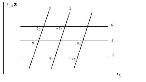
FIG. 3.: Diagonal elements of the Hamiltonian (25) as functions of time.

Let $P_{ij}$ ($i,j=1,...,6$) be the probability to transit from the state $j$ to the state $i$ after the band crossing. The transition probabilities can be expressed in terms of the fermi-operators in the Heisenberg representation at $t\rightarrow\infty$.

$$\begin{array}[]{l}P_{1n}=<n|\hat{a}^{+}\hat{a}\hat{d}^{+}\hat{d}|n>\\ P_{2n}=<n|\hat{b}^{+}\hat{b}\hat{d}^{+}\hat{d}|n>\\ P_{3n}=<n|\hat{c}^{+}\hat{c}\hat{d}^{+}\hat{d}|n>\\ P_{4n}=<n|\hat{a}^{+}\hat{a}\hat{b}^{+}\hat{b}|n>\\ P_{5n}=<n|\hat{a}^{+}\hat{a}\hat{c}^{+}\hat{c}|n>\\ P_{6n}=<n|\hat{b}^{+}\hat{b}\hat{c}^{+}\hat{c}|n>\\ \end{array}$$ (26)

Substituting (24) into (26) and employing the elements of the evolution matrix from (17) we get the following result:

$$P=\left(\begin{array}[]{llllll}p_{2}p_{3}&q_{1}q_{2}p_{3}&q_{1}q_{3}&p_{1}q_{2}p_{3}&p_{1}q_{3}&0\\ 0&p_{1}p_{3}&p_{1}q_{2}q_{3}&q_{1}p_{3}&q_{1}q_{2}q_{3}&p_{2}q_{3}\\ 0&0&p_{1}p_{2}&0&q_{1}p_{2}&q_{2}\\ q_{2}&q_{1}p_{2}&0&p_{1}p_{2}&0&0\\ p_{2}q_{3}&q_{1}q_{2}q_{3}&q_{1}p_{3}&p_{1}q_{2}q_{3}&p_{1}p_{3}&0\\ 0&p_{1}q_{3}&q_{2}p_{3}p_{1}&q_{1}q_{3}&q_{1}q_{2}p_{3}&p_{2}p_{3}\end{array}\right)$$ (27)

where

$$\begin{array}[]{l}p_{i}=e^{-2\pi|g_{i}|^{2}}\\ q_{i}=1-p_{i},\,\,\,(i=1,2,3)\end{array}$$ (28)

V Conclusions.

In conclusion, we presented the procedure that generates new exactly solvable multi-state LZ models. Some of them are useful for the description of driven charge transport in quantum dots and driven tunneling in nanomagnets. As an example, we derived two new solvable models and found the transition probability matrices for them.

There have been three known classes of solvable multi-state LZ models that provide transition probabilities for a finite number of states:

1. The Demkov-Osherov model.

2. The $SU(2)$ symmetry class that deals with an arbitrary spin in external magnetic field with the following Hamiltonian:

   $$\hat{H}=t\hat{S}_{z}+g\hat{S}_{x}$$ (29)

3. The generalized bow-tie model that treats the case when two levels are parallel while the other levels intersect at one point between the parallel ones.

This list can be extended with different generalizations of these models to the case of degenerate states. For example, it is possible to solve the LZ model for two degenerate levels by changing basis in such a way that all equations decouple into independent two state Landau-Zener transitions. It is worth mentioning that sometimes a few elements of transition probability matrix can be found while the others remain unknown [9], [19].

All these models provide very simple results. For example, transition probabilities in the Demkov-Osherov model coincide with those taken from successive application of the two state Landau-Zener formula. The same is true for the generalized bow-tie model. Finally in all models the transition probabilities are simple polynomials of $z_{k}=\exp(-\pi|g_{k}|^{2})$. This fact gives a strong feeling that there should be a common symmetry in the background of all these models. Our results demonstrate the same properties and we know that the reason for this was the symmetry that makes the Hamiltonian equivalent in some sense to the one for a much simpler problem.

We did not study deeply the relations between the known models and our new solutions but there are indications that such a relation can exist. For example the model (5) and the generalized bow-tie model are very similar. At $g=\gamma$ and $\beta_{1}=-\beta_{2},\,\beta_{3}=-\beta_{4}$ the Hamiltonian (5) belongs to the class of generalized bow-tie models. Also we note that models of $SU(2)$ class [13] can be derived from the following bosonic Hamiltonian:

$$\hat{H}=t\hat{a}^{+}\hat{a}-t\hat{b}^{+}\hat{b}+g(\hat{a}^{+}\hat{b}+\hat{b}^{+}\hat{a})$$ (30)

In the single-particle sector the Hamiltonian (30) leads to the simple two-state LZ model. In the $N$-boson sector the Schrödinger equation for diabatic states coincides with ones for a spin $S=N/2$ in magnetic fields. This construction is an application of the Schwinger bosons [23] to the LZ problem.

It is interesting to check what models can be reduced to decoupled two level systems. Probably this can be done using of the group representation theory.

REFERENCES

• [1] L.D.Landau, Physik Z. Sowjetunion 2, 46 (1932)
• [2] C.Zener, Proc. Roy. Soc. Lond. A 137, 696 (1932)
• [3] D. A. Harmin, P. N. Price, Phys. Rev. A. 49 (1994) 1933
• [4] E.E. Nikitin, S. Ya Umanskii ”Theory of Slow Atomic Collisions”,
• [5] R. Giraud, W. Wernsdorfer, A.M.Tkachuk, D. Mailly, B. Barbara, cond-mat/0102231
• [6] V.A. Yurovsky, A. Ben-Reuven, P. S. Julienne Phys. Rev. A. V65, 043607 (2002)
• [7] Yu. Gefen, E. Ben-Jacob, A. O. Caldeira, Phys. Rev. B. 36 (1987) 2770-2782
• [8] D. Iliescu, S. Fishman, E. Ben-Jacob, Phys. Rev. B, 46 (1992) 675-685
• [9] S. Brundobler, V. Elser, J. Phys. A: Math.Gen. 26 (1993) 1211-1227
• [10] Yu. N. Demkov, V. N. Ostrovsky, J. Phys. B: At. Mol. Opt. Phys. 28 (1995) 403-414
• [11] V.N. Ostrovsky, H. Nakamura, J.Phys A: Math. Gen. 30 6939-6950(1997)
• [12] Y.N. Demkov, V.N. Ostrovsky, J. Phys. B. 34 (12), (2001) 2419-2435
• [13] F.T. Hioe, J. Opt. Soc. Am. B 4, 1237-1332 (1987)
• [14] C.E. Carroll, F. T. Hioe, J. Phys. A: Math. Gen. 19, 1151-1161 (1986)
• [15] V.A. Yurovsky, A. Ben-Reuven, Phys. Rev. A. V63, 043404 (2001)
• [16] Y. N. Demkov, V.N. Ostrovsky, Phys. Rev. A 61, 032705 (2000)
• [17] V.L. Pokrovsky, N.A. Sinitsyn, Phys. Rev. B 65, 153105 (2002)
• [18] Yu. N. Demkov, V. I. Osherov, Zh. Exp. Teor. Fiz. 53 (1967) 1589 (Engl. transl. 1968 Sov. Phys.-JETP 26, 916)
• [19] T. Usuki, Phys.Rev.B 56, 13360 (1997)
• [20] E. Bauer, E. A. Fisher, J. Chem. Phys. 51 (1972) 1966
• [21] F. Renzoni, T. Brandes, Phys. Rev. B 64 (2001) 245301, cond-mat/0109335 chapter 10, Springer-Verlag, 1984
• [22] Yu. N. Demkov, P.B. Kurasov, V.N. Ostrovsky, J.Phys. A: Math. Gen. (1995) 4361-4380
• [23] J. Schwinger, unpublished notes. See, for example, J.J. Sakurai, Modern Quantum Mechanics, Addison-Wesley, Reading, 1994.