Fast noise in the Landau-Zener theory.

Abstract

We study the influence of a fast noise on Landau-Zener transitions. We demonstrate that a fast colored noise much weaker than the conventional white noise can produce transitions itself or can change substantially the Landau-Zener transition probabilities. In the limit of fast colored or strong white noise we derive asymptotically exact formulae for transition probabilities and study the time evolution of a spin coupled to the noise and a sweeping magnetic field.

I Introduction

Landau-Zener (LZ) formula for transition probabilities at avoided crossing of two levels is one of a few fundamental results of non-stationary quantum mechanics. Its rather general character and simplicity makes it extremely suitable for versatile applications. Traditionally it was applied in quantum chemistry chemistry and in collision theory inc , nik . A recent treatment of the experiments on the quantum molecular hysteresis in nanomagnets by Wernsdorfer and Sessoli WS1 ; WS2 ; nm was a real triumph of the LZ theory. A substantial contributions to the theory of spin tunnelling in these molecules was made by theorists Garg ; GC ; Prokofev . Landau-Zener formula and its generalizations were recently employed also for charge transport in nanostructures av1 ; av2 ; Gef ; Iliescu ; dot2 , Bose-Einstein condensates Y1 and quantum computing FG .

Extensions of the LZ theory to the case of multilevel crossing are less general. Nevertheless, some of them were realistic enough to justify remarkable efforts on the side of theorists for their analysis. Level correlations and localization in energy space were studied in Gef-loc . The pioneering work by Demkov and Osherov demkov treated exactly the crossing of a single level with a band of parallel levels. In the work zeeman2 Hioe and Carrol solved a problem of transitions in a Zeeman multiplet of an arbitrary spin S in a magnetic field with a constant perpendicular component and a time-dependent parallel component passing through zero value. Numerous generalizations of these results were found brand ; deminf1 ; bow ; dem33 ; zeeman1 ; dem3 ; PS ; usuki . A general point of view on all these exactly solvable models proposed by one of authors sinitsyn allowed to construct an algorithm for series of new solvable models. Another extensions include nonlinear LZ-model Liu ; Liu2 ; Zob and LZ problem with nonlinear sweep Garanin . To apply the LZ formula and its multi-state extensions to real systems it is often necessary to take into account the interaction with environment. Such attempts were made in a series of works GC ; Sai ; kay4 ; Kay ; kay3 ; Nish ; SaiKay ; Ao ; Kob ; Shi ; Kay2 ; Loss ; Ben ; Usuki2 , however the problem was not solved completely. Kayanuma et al. Sai ; kay4 ; Kay have obtained an elegant analytic result for the diagonal white noise. The non-diagonal colored noise was considered by Kayanuma kay3 for the two-level crossing without a constant coupling term. He has found the transition probability in the limit of infinitely short noise correlation time. His result was disputed by Nishino et al. Nish . On the basis of their numerical calculations these authors concluded that the transitions due to non-diagonal noise are weak in many realistic situations. The discrepancy is associated with different limiting procedures in calculations. In the limit of infinitely short correlations but finite amplitude of sweeping field the transition probability was found to be vanishingly small.

The influence of the noise onto the multilevel crossing was studied so far in only one work by Saito and Kayanuma SaiKay , who considered the 3-level crossing at a special relations between parameters in the limit of strong decoherence.

The purpose of this article is to present a systematic study of the influence of noise, including the colored noise, onto the LZ transitions and to generalize it to multistate LZ problems. We demonstrate that the LZ transitions are sensitive to the colored noise much weaker than usual $\delta$-like white noise. The latter can be considered as a limit of a noise whose correlation time goes to zero and simultaneously its square of amplitude goes to infinity, so that their product remains a constant. We prove that such a white non-diagonal noise always leads to equal population of the crossing levels. However, the noise, whose correlation time goes to zero, but its amplitude remains a constant, produces non-trivial transition probabilities as it was first found by Kayanuma kay3 for a special type of the noise correlation function. Another subtle problem is the order of limiting processes Nish . The resulting probabilities depend crucially on what happens first: time asymptotically goes to infinity or correlation time goes to zero. Analysis of these problems allowed us to reconcile works kay3 and Nish . In our work we first find simple analytical result for a transition produced by a most general short-time correlated noise in 2-level systems and the change of the LZ probabilities produced by such a noise. We check these analytical results by numerical calculations. We also study the influence of the noise on transitions at multilevel crossing.

The plan of the article is as follows. In section II we generalize the result of Kayanuma for transverse noise kay3 to the case of the arbitrary Gaussian noise in all three directions. Next we demonstrate its generalization to a three level system. In the section IV we study the time dependence of the density matrix with LZ transitions stimulated by fast noise. In the fifth section we propose a formula that incorporates constant transverse magnetic field and compare its predictions with numerical simulations. In section VI we consider the master equation for an arbitrary spin placed into a regular varying field and noisy magnetic field along the $z$-direction and a constant field along $x$-direction and find simple expressions for transition probabilities in the limit of a strong decoherence. In section VII we perform similar calculations for a charged particle on a periodic chain driven by a time-dependent electric field and compare our results with those for a completely coherent evolution.

II Colored noise in two level LZ transitions.

LZ transitions in a two-level system with a non-diagonal noise were studied by Kayanuma in kay3 . The Hamiltonian of the problem was chosen to be

$$H=\beta t\sigma_{z}+\eta_{x}\sigma_{x}$$ (1)

where $\eta_{x}$ is the noise field with the correlation function $\langle\eta_{x}(t_{1})\eta_{x}(t_{2})\rangle=J_{x}^{2}e^{-\lambda_{x}|t_{1}-t_{2}|}$ and $\sigma_{i}$ are Pauli matrices. In the limit of infinitely short correlation time $\lambda\rightarrow\infty$ Kayanuma has found a simple analytical result for the transition probability.

The choice of Kayanuma corresponds to the spin $1/2$ problem with noisy magnetic field along the $x$-axes only. We generalize the Kayanuma model introducing a more general Hamiltonian with all 3 components of random magnetic field being non-zero and with a most general form of the short-time correlation tensor:

$$H=\beta t\sigma_{z}+\sum_{i}\eta_{i}(t)\sigma_{i},\,\,i=x,y,z$$ (2)

$$\langle\eta_{i}(t_{1})\eta_{j}(t_{2})\rangle=g_{ij}(\lambda|t_{1}-t_{2}|)$$ (3)

We assume that though $g_{ij}$ can be different for different $i,j$, they are of the same order of magnitude. We consider the limit of fast noise with $\lambda\rightarrow\infty$, where $\lambda$ is the inverse characteristic decay time of the correlator $g_{ij}$.

The density matrix elements for the system with the Hamiltonian (1) obey the following system of ordinary differential equations:

$$\begin{array}[]{l}i\dot{\rho}=2(-\rho_{12}(\eta_{x}-i\eta_{y})+\rho_{21}(\eta_{x}+i\eta_{y}))\\ i\dot{\rho}_{12}=2(\beta t+\eta_{z})\rho_{12}-\rho(\eta_{x}+i\eta_{y})\\ i\dot{\rho}_{21}=-2(\beta t+\eta_{z})\rho_{21}+\rho(\eta_{x}-i\eta_{y})\end{array}$$ (4)

where $\rho=\rho_{11}-\rho_{22}$. By elimination of non-diagonal matrix elements equations (4) are transformed into one integral-differential equation for the occupation difference $\rho$:

$$\begin{array}[]{l}\frac{d\rho(t)}{dt}=-2e^{-i\beta t^{2}}(\eta_{x}(t)-i\eta_{y}(t))\int_{-\infty}^{t}dt_{1}e^{i\beta t_{1}^{2}-i\int_{t_{1}}^{t}\eta_{z}(t_{2})dt_{2}}(\eta_{x}(t_{1})+i\eta_{y}(t_{1}))\rho(t_{1})\\ -2e^{i\beta t^{2}}(\eta_{x}(t)+i\eta_{y}(t))\int_{-\infty}^{t}dt_{1}e^{-i\beta t_{1}^{2}+i\int_{t_{1}}^{t}\eta_{z}(t_{2})dt_{2}}(\eta_{x}(t_{1})-i\eta_{y}(t_{1}))\rho(t_{1})\end{array}$$ (5)

The solution of this equation can be formally found as an infinite series in powers of $\eta_{i}$ that must be averaged over noise realizations. A typical term contains the product $\eta_{i_{1}}(t_{1})\eta_{i_{2}}(t_{2})\ldots\eta_{i_{n}}(t_{n})$. Its average is equal to the sum of all possible products of pair correlators since we assume the noise to be Gaussian. Kayanuma kay3 has shown that in the limit of very fast noise only the term in which the pairing is ideally ordered in time, i.e. the pairs are (12)(34)…(2n-1,2n), contributes a finite value into the integral. Other pairings contribute terms, which are by a power of infinitely small parameter $1/\lambda$ smaller and can be neglected. This Kayanuma’s observation is completely analogues to the theorem proven by Abrikosov and Gor’kov in their theory of impurities in a metal AbrGor . Note that the diagonal component of noise is inessential in this approximation and can be omitted. These facts allow to write down the integral-differential equation for the average value of $\rho$ as follows:

$$\frac{d\langle\rho\rangle(t)}{dt}=-4\int_{-\infty}^{t}\cos\left(\beta(t^{2}-t_{1}^{2})\right)F\left(\lambda|t-t_{1}|\right)\langle\rho\rangle(t_{1})dt_{1}$$ (6)

where $F=g_{xx}+g_{yy}$. Now we can employ the approximation of the fast noise assuming that the average $\langle\rho\rangle(t)$ almost does not change in the interval of time $1/\lambda$ and that integral of correlation function is convergent. In this approximation we can extract $\langle\rho\rangle(t)$ from the integral in the right-hand side of equation (6) and expand the argument of the cosine near the end point $t_{1}=t$ of the integral. The resulting differential equation reads:

$$\frac{d\langle\rho\rangle}{dt}=-4\hat{F}(2\beta t)\langle\rho\rangle$$ (7)

where $\hat{F}(q)$ is the cosine Fourier transform of the function $F$:

$$\hat{F}(q)=\int_{-\infty}^{\infty}\cos(q\tau)F(\lambda|\tau|)d\tau$$ (8)

Note that the characteristic value of $q$ are of the order $\lambda$ and, respectively, essential values of $t$ in equation (7) are $t\sim\lambda/\beta$. We see that essential values of time go to infinity together with $\lambda$. It shows that the order of limiting processes is indeed very important. Here we first calculate the transition probability, i.e. the diagonal elements of the density matrix at $t=\infty$ and at very large, but still finite $\lambda$ and put it infinity in the end. Solving equation (7), we find:

$$\langle\rho\rangle(t)=\langle\rho\rangle(-\infty)\exp\left(-4\int_{-\infty}^{t}\hat{F}(2\beta t^{\prime})dt^{\prime}\right)$$ (9)

Together with the standard equation $\rho_{11}+\rho_{22}=1$ equation (9) determines average occupation number of each level at any time. The most interesting are the transition probabilities at $t=+\infty$, which can be obtained from the same equation (9). Note that the integral in the exponent at $t=+\infty$ becomes equal to

$$\int_{-\infty}^{\infty}\hat{F}(2\beta t^{\prime})dt^{\prime}=\frac{\pi}{2\beta}F(0)$$ (10)

Thus, from equations (9) and (10) we find:

$$\rho_{11}(+\infty)=\frac{1}{2}\left[1+\left(2\rho_{11}(-\infty)-1\right)\exp\left(-\frac{2\pi F(0)}{\beta}\right)\right];$$ (11)

$$\rho_{22}(+\infty)=\frac{1}{2}\left[1-\left(2\rho_{11}(-\infty)-1\right)\exp\left(-\frac{2\pi F(0)}{\beta}\right)\right]$$ (12)

Putting $\rho_{11}(-\infty)=1$, we find the transition probability:

$$P_{1\rightarrow 2}=\rho_{22}(+\infty)\mid_{\rho_{11}(-\infty)=1}=\frac{1}{2}\left[1-\exp\left(-\frac{2\pi F(0)}{\beta}\right)\right]$$ (13)

For the standard white noise the correlators $\langle\eta_{i}(t)\eta_{j}(t^{\prime})\rangle$ turn into delta-functions in the limit $\lambda=\infty$. It means that their values at $t=t^{\prime}$ become infinitely large. In particular it means that $F(0)$ is infinitely large for the standard white noise. In this case, as it is seen from equations (11), (12) the occupancies of both levels are equal to 1/2. Thus, the standard white noise leads to complete loss of initial state memory and equipartition of the levels. On the other hand, if the amplitude of noise remains finite, the occupation numbers conserve memory on the initial state.

In the limit of the fast noise the transition probabilities are determined only by the average square of non-diagonal noise and are not sensitive to the diagonal noise. To illustrate this statement we consider a special case when the diagonal noise does not correlate with the non-diagonal one. Then, as it is seen from equation (5), the averaging over the $z$-component of the noise leads to multiplication of the coefficients in this integral-differential equation by the Debye-Waller factor

$$\langle\exp\left(\int_{t_{1}}^{t}\eta_{z}(\tau)d\tau\right)\rangle$$

$$=exp\left(-\frac{1}{2\lambda}(t-t_{1})\int_{-\infty}^{\infty}g_{zz}(\theta)d\theta\right)$$

An essential interval of integration over $t_{1}$ near $t_{1}=t$ is $1/\lambda$. In this interval the Debye-Waller factor changes by the value $\sim 1/(\lambda)^{2}$ and with this precision is equal to 1.

For a special case $g_{xx}(\tau)=J^{2}\exp(-\lambda|\tau|);g_{yy}(\tau)=0$ we reproduce the Kayanuma’s result kay3 .

III Nondiagonal noise in spin-1 LZ theory.

The Hamiltonian $H$ of a general multi-state LZ problem (see for example brand ) has the following matrix form

$$H=Bt+A,$$ (14)

where $B$ is a diagonal matrix and matrices $A$ and $B$ are independent on time. However, in a situation of a general position only two levels cross. Several levels can intersect at the same moment of time only due to a special symmetry. Such a symmetry is systematically realized in the model of an arbitrary spin $S\neq 1/2$ placed into an external magnetic field that has a time-dependent $z$-component vanishing at some moment of time $t=0$ and a constant transverse component zeeman2 . The corresponding Hamiltonian is:

$$H=\beta tS_{z}+gS_{x}$$ (15)

where $\beta$ and $g$ are constants. This exactly solvable model for a spin higher than $1/2$ was employed in the theory of Stark effect Kaz ; some recent applications can be found in agu ; Suo .

In this section we generalize the result (13) to a spin 1 system. We consider a following Hamiltonian for the spin 1 system in a random magnetic field:

$$H=(\beta t)S_{z}+\sum_{i=-1}^{+1}\eta_{i}S_{i}$$ (16)

where $S_{i}$ are the spin projection operators for $S=1$. The density matrix $\rho$ depends on 8 independent parameters. We denote $\rho_{+}=\rho_{1,1}-\rho_{0,0}$ and $\rho_{-}=\rho_{-1,-1}-\rho_{0,0}$. The derivation of equations for $\rho_{+}$ and $\rho_{-}$ can be done in the same spirit as it was done for the spin $1/2$ case. Looking for a solution of the evolution equation for density matrix in the form of perturbation series and retaining after the averaging over the noise only the leading terms in $1/\lambda$, we arrive at an integral-differential equation. Additional care must be paid to the integrals of the form $\int_{-\infty}^{t}dt_{1}\int_{-\infty}^{t_{1}}dt_{2}\exp(i\beta(t_{1}^{2}+t_{2}^{2}))g_{ij}(\lambda|t_{1}-t_{2}|)$ that did not appear in the two level system, but appeared in the series for the spin $S=1$. One can check that this integral is of the order $1/\lambda$ and hence we disregard it and all terms that contain it. After lengthy but straightforward calculations we find that in the leading order in $1/\lambda$ the elements $\rho_{+}(t)$ and $\rho_{-}(t)$ satisfy the following integral-differential equation:

$$\frac{d}{dt}\begin{array}[]{l}\left(\begin{array}[]{l}\rho_{+}(t)\\ \rho_{-}(t)\end{array}\right)=-2\int_{-\infty}^{t}dt_{1}\cos(\beta(t^{2}-t_{1}^{2})/2)F(\lambda|t-t_{1}|)\left(\begin{array}[]{cc}1&1/2\\ 1/2&1\end{array}\right)\left(\begin{array}[]{c}\rho_{+}(t_{1})\\ \rho_{-}(t_{1})\end{array}\right)\end{array}$$ (17)

The approximation of the fast noise allows to transform this equation into the following differential one:

$$\frac{d}{dt}\left(\begin{array}[]{l}\rho_{+}(t)\\ \rho_{-}(t)\end{array}\right)=-2\hat{F}(\beta t)\left(\begin{array}[]{cc}1&1/2\\ 1/2&1\end{array}\right)\left(\begin{array}[]{c}\rho_{+}(t_{1})\\ \rho_{-}(t_{1})\end{array}\right)$$ (18)

Thus, the problem is reduced to a linear differential equation with a constant matrix coefficient. The formal answer is:

$$\left(\begin{array}[]{l}\rho_{+}(t)\\ \rho_{-}(t)\end{array}\right)=\exp\left[-2\int_{-\infty}^{t}\hat{F}(\beta|\tau|)d\tau\left(\begin{array}[]{cc}1&1/2\\ 1/2&1\end{array}\right)\right]\left(\begin{array}[]{l}\rho_{+}(-\infty)\\ \rho_{-}(-\infty)\end{array}\right)$$ (19)

This formal solution can be transformed to a more explicit form with the help of the matrix identity:

$$\exp\left[-\gamma\left(\begin{array}[]{cc}1&1/2\\ 1/2&1\end{array}\right)\right]=e^{-\gamma}\left(\begin{array}[]{cc}\cosh\gamma/2&-\sinh\gamma/2\\ -\sinh\gamma/2&-\cosh\gamma/2\end{array}\right)$$ (20)

The transition probabilities are defined by this matrix acting on vectors $\left(\begin{array}[]{l}1\\ 0\end{array}\right)$ if initially the projection $+1$ was occupied , or $\left(\begin{array}[]{l}0\\ 1\end{array}\right)$ if the projection $-1$ was occupied. The transition probabilities are:

$$\begin{array}[]{l}P_{+\rightarrow 0}=P_{-\rightarrow 0}=\frac{1}{3}\left(1-e^{-3\gamma/2}\right)\\ P_{+\rightarrow+}=P_{-\rightarrow-}=\frac{1}{3}+\frac{1}{6}e^{-3\gamma/2}+\frac{1}{2}e^{-\gamma/2}\\ P_{+\rightarrow-}=P_{-\rightarrow+}=\frac{1}{3}+\frac{1}{6}e^{-3\gamma/2}-\frac{1}{2}e^{-\gamma/2}\\ P_{0\rightarrow 0}=\frac{1}{3}\left(1+e^{-3\gamma/2}\right)\\ P_{0\rightarrow+}=P_{0\rightarrow-}=\frac{1}{3}\left(1-e^{-3\gamma/2}\right)\end{array}$$ (21)

where $\gamma=\pi F(0)/\beta$.

We see that in the case of 3 levels the main results obtained in the previous section for a 2-level system persist: the standard white ($\gamma=\infty$) noise leads to equal population of all 3 levels, whereas the fast noise with a finite amplitude results in non-trivial transition probabilities.

IV Transition time for colored noise

In section 2 we have shown that the typical time for establishing the asymptotic of the transition probabilities is $\lambda/\beta F(0)$. It is useful to look at the same problem from a different point of view. Namely, we will analyze the behavior of transitions driven by the standard $\delta$-like white noise, their typical rates and times. If the action of the standard white noise is limited by some finite time interval, it becomes physically equivalent to the fast noise with a finite amplitude. Simultaneously we will study directly the influence of the white noise onto the LZ transitions.

Let us consider the problem with the very beginning. The Hamiltonian is the generator of a random rotation:

$$H={\bf h(t)S}$$ (22)

where ${\bf h}(t)={\bf h}_{0}(t)+{\bf\eta}(t)$ and ${\bf h_{0}}(t)=\beta t\hat{z}+\Gamma\hat{x}$. Here we consider the isotropic white noise $\langle\eta_{i}(t)\eta_{k}(t^{\prime})\rangle=\gamma\delta_{ik}\delta(t-t^{\prime})$.
The density matrix as any Hermitian $S\times S$ matrix can be represented as a sum:

$${\bf\rho}=\rho^{(0)}I+\rho_{i}^{(1)}S_{i}+\rho_{ik}^{(2)}\left[S_{i}S_{k}+S_{k}S_{i}-\frac{2}{3}S(S+1)\right]+...$$ (23)

where the last term in equation (29) contains $S$ operator factors. All irreducible tensors $\rho^{(j)};\,\,j=0...S$ evolve separately. The scalar $\rho^{(0)}=(1/N)Tr\rho$ is a constant. The vector ${\bf\rho}^{(1)}$ obeys an obvious equation:

$$\dot{{\bf{\rho}}^{(1)}}=-{\bf h}\times\bf{\rho}^{(1)}$$ (24)

The modulus of the vector $\vec{\rho}^{(1)}$ is conserved.

Dynamic equation for the 2-nd order symmetric tensor $\rho_{ik}$ reads:

$$\dot{\rho}_{ik}=-\epsilon_{imn}h_{m}\rho_{nk}-\epsilon_{kmn}h_{m}\rho_{in}$$ (25)

The extension for the rest of irreducible components is obvious. In equation (24) for the vectorial part it is useful to apply the interaction representation: $\bf{\rho}^{(1)}(t)=U_{0}(t,t_{0})\tilde{\bf{\rho}}^{(1)}(t)$, where $U_{0}(t,t_{0})$ is the evolution matrix for the field ${\bf h}_{0}(t)=\hat{z}\beta t+\hat{x}\Gamma$. The reduced vector $\tilde{\bf{\rho}}^{(1)}(t)$ obeys the following equation:

$$\frac{d}{dt}\tilde{\bf\rho}^{(1)}(t)=-\tilde{\bf\eta}\times\tilde{\bf\rho}^{(1)}(t)$$ (26)

Here $\tilde{\bf\eta}=U_{0}^{-1}({\bf\eta}\times U_{0})$. In terms of the Cartesian coordinates this equation reads:

$$\dot{\tilde{\rho}}_{i}=T_{ikl}\tilde{\rho}_{k}\eta_{l}$$ (27)

where the matrix $T_{ikl}$ is:

$$T_{ikl}(t,t_{0})=(U_{0})_{mi}(U_{0})_{nk}\epsilon_{mln}$$ (28)

Initial values of ${\bf\rho}$ and $\tilde{\bf\rho}$ coincide since $U_{0}(t_{0},t_{0})=I$. Equation (27) can be solved by power expansion over the noise:

$$\tilde{\rho}_{i}(t)=\rho_{i}(t_{0})+\int_{t_{0}}^{t}T_{ikl}(t^{\prime},t_{0})\eta_{l}(t^{\prime})dt\rho_{k}(t_{0})+...$$ (29)

When averaging the expansion over the noise, all odd terms vanish. To understand what happens with even terms consider first the quadratic term:

$$\int_{t_{0}}^{t}dt_{1}\int_{t_{0}}^{t_{1}}dt_{2}T_{ik_{1}l_{1}}(t_{1},t_{0})T_{k_{1},k,l_{2}}(t_{2},t_{0})\langle\eta_{l_{1}}(t_{1})\eta_{l_{2}}(t_{2})\rangle\rho_{k}(t_{0})$$

For the isotropic noise the contribution to the vector $\tilde{\bf\rho}(t)$ up to the second order in ${\bf\eta}$ can be represented as follows (we write equations for averages omitting the angular brackets):

$$\tilde{\rho}_{2,i}(t)=\left(\delta_{ik}+\int_{t_{0}}^{t}dt_{1}M_{ik}(t_{1})\right)\rho_{k}(t_{0})$$ (30)

where

$$M_{ik}(t)=(\gamma/2)T_{iml}(t,t_{0})T_{mkl}(t,t_{0})=-\gamma\delta_{ik}$$ (31)

Here we have used properties of the orthogonal matrices $U_{0}$: $(U_{0})_{mi}(U_{0})_{mk}=\delta_{ik}$.

Next we proceed to the quartic term:

$$\tilde{\rho}_{4,i} = \int_{t_{0}}^{t}dt_{1}\int_{t_{0}}^{t_{1}}dt_{2}\int_{t_{0}}^{t_{2}}dt_{3}\int_{t_{0}}^{t_{3}}dt_{4}T_{ipk}(t_{1},t_{0})T_{pql}(t_{2},t_{0})T_{qrm}(t_{3},t_{0})T_{rsn}(t_{4},t_{0})$$ (32)

$$\times \langle\eta_{k}(t_{1})\eta_{l}(t_{2})\eta_{m}(t_{3})\eta_{n}(t_{4})\rangle\rho_{s}(t_{0})$$

Quartic average of Gaussian field decays into quadratic averages:

$$\langle\eta_{k}(t_{1})\eta_{l}(t_{2})\eta_{m}(t_{3})\eta_{n}(t_{4})\rangle=\langle\eta_{k}(t_{1})\eta_{l}(t_{2})\rangle\langle\eta_{m}(t_{3})\eta_{n}(t_{4})\rangle$$

$$+\langle\eta_{k}(t_{1})\eta_{m}(t_{3})\rangle\langle\eta_{l}(t_{2})\eta_{n}(t_{4})\rangle+\langle\eta_{k}(t_{1})\eta_{n}(t_{4})\rangle\langle\eta_{l}(t_{2})\eta_{m}(t_{3})\rangle$$ (33)

Only the first term contributes to the integral (32). Two others are zero at correct time ordering $t_{1}\geq t_{2}\geq t_{3}\geq t_{4}$. In both cases considered earlier we obtain:

$$\tilde{\rho}_{4,i}=\int_{t_{0}}^{t}dt_{1}\int_{t_{0}}^{t_{1}}dt_{2}M_{ij}(t_{1})M_{jk}(t_{2})\rho_{k}(t_{0})$$ (34)

The same result could be obtained from an effective equation of motion for $\tilde{\rho}$:

$$\dot{\tilde{\rho}}_{i}=M_{ik}\tilde{\rho}_{k}$$ (35)

Thus, the operator ${\bf M}$ plays the role of effective non-Hermitian Hamiltonian.

For the white isotropic noise the solution of the equation (35) is:

$$\tilde{\rho}_{i}(t)=\tilde{\rho}_{i}(t_{0})exp(-\gamma t)$$ (36)

At $t\rightarrow\infty$ the formula (36) always leads to the occupation numbers $p=1/2$. As we know, this does not happen for the colored noise with a finite amplitude. The reason is that in the genuine LZ problem the solution strongly oscillates with the frequency roughly $\omega(t)\sim\beta t$ long before and after the level crossing point. This introduces a new energy scale that must be compared with $\lambda$. For time in the range $|\beta t|<\lambda$, the approximation of white noise is roughly valid even for finite amplitude noise, but beyond this interval of time the oscillations of the LZ solution become faster than the correlation time of the noise, and the action of the noise is suppressed by the oscillations.

In $Fig.1$ we demonstrate a typical evolution of the probability for the system to stay in the same state as a function of time. The evolution reminds diffusive motion that slowly stops at large absolute values of time. The sharp change of the absolute value of the amplitude near $t=0$ is due to the constant transverse field.

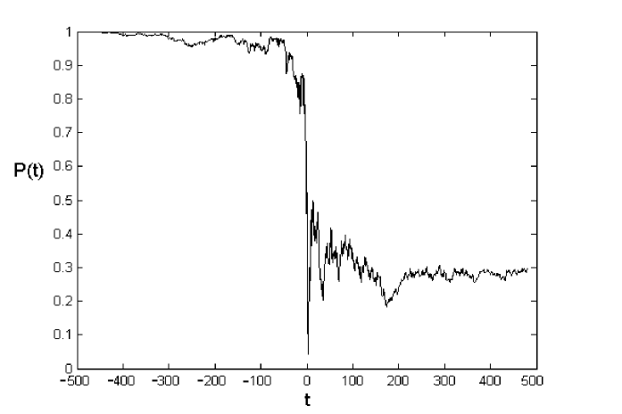
Figure 1: Typical evolution of the probability $P(t)=|a_{1}(t)|^{2}$, where $a_{1}(t)$ is the amplitude of the first diabatic state. The choice of parameters is as follows, $g_{ij}=\delta_{ij}J^{2}e^{-\lambda|t-t^{\prime}|}$, $\beta=1$, $\lambda=80$, $J^{2}=0.18$, $\Gamma=0.7$.

To estimate roughly the transition probability one can apply the standard white noise approximation in the time interval $|t|<C\lambda/\beta$ and accept that at $|t|>C\lambda/\beta$ no transitions due to the noise happen. The parameter $C$ is a constant of the order of unity. Then we automatically get the result $\rho(\infty)=\exp(-2C\lambda\gamma/\beta)\rho(-\infty)$. According to the definition, $\gamma\approx F(0)/\lambda$ in agreement with the calculations of the previous sections. Summarizing, the transitions mediated by the fast noise proceed during the large time interval of the order of $\lambda/\beta$. This is the reason why its total effect remains finite, though it is very small on a typical time scale of the usual LZ-transitions mediated by constant field ($\tau\sim\Gamma/\beta$) Gef-time .

V Landau-Zener transitions in a constant transverse field and in the colored noise.

In previous sections we assumed that only the noise was responsible for transitions, whereas the regular part of the Hamiltonian operator was diagonal. In this section we incorporate a regular non-diagonal operator (the transverse field) into the Hamiltonian together with a noise. The most general Hamiltonian for such a two-level system reads:

$$H=\beta t\sigma_{z}+g\sigma_{x}+\sum_{i}\eta_{i}(t)\sigma_{i},\,\,i=x,y,z$$ (37)

where $\eta_{i}$ are coordinates of the vectorial Gaussian noise with correlators given by (3).

The second term in the Hamiltonian (37) can be considered as a constant transverse magnetic field acting on a spin $S=1/2$. The Hamiltonian (37) describes a spin (q-bit) weakly interacting with the environment, for example with the nuclear spin bath PS . If this interaction is so small that the bath relaxation is much faster than the inverse interaction energy, the bath can be treated as a fast noisy magnetic field. The measurements of the LZ transition probabilities can provide an information about the strength of the coupling to the bath. Another possible example is a molecular nanomagnet in fluctuating dipole field. The Hamiltonian (37) may be relevant to the quantum shuttle problem where avoided level crossings occurred to be important shuttle . The fast noise in this example corresponds to thermal fluctuations.

As it was discussed in the previous section, in the interval of time $|\beta t|<<\lambda$ the spin experiences an equivalent white noise with the amplitude $\gamma=F(0)/(2\lambda)$ vanishing at $\lambda\rightarrow\infty$. The noise causes a slow decay of the population difference $\rho=\rho_{11}-\rho_{22}$. The action of the noise becomes noticeable only after long evolution time of the order $|\lambda/\beta|$. On the contrary, the transitions due to the constant transverse field proceed predominantly during a much shorter interval of time $|t|<|g/\beta|$. During this interval of time the role of noise is negligible comparing with the role of the constant transverse field. Let us choose $t_{0}$ much less than $|\lambda/\beta|$, but much larger than $g/\beta$ to make sure that the transverse magnetic field is neglegible beyond the interval of time $(-t_{0},t_{0})$. The evolution from $-\infty$ to $-t_{0}$ is influenced mainly by the noise. The result of such an evolution is almost the same as that in the absence of the constant transverse field with $t_{0}=0$. Since the effective attenuation coefficient for $\rho$ is an even function of time (see equation (7)), the resulting exponent for $\rho(t_{0})$ is twice less than that for the problem of the section (2) at $t=+\infty$ (equations (9,10):

$$\rho(-t_{0})=e^{-\pi F(0)/\beta}$$ (38)

In the interval of time $|t|<t_{0}$ the noise is neglegible and transitions are completely due to the genuine Landau-Zener mechanism, i.e. due to the constant transverse field $g$. Since $t_{0}\gg g/\beta$, we can use the LZ formula to determine $\rho(t_{0})$. Let $a_{1}(t)$ and $a_{2}(t)$ be the amplitudes to find the system at the first and the second diabatic states, respectively, (to find the spin projection equals $1/2$ or $-1/2$) at the moment of time $t$. Their values at $t=-t_{0}$ can be expressed in terms of the population difference $\rho^{*}$ and two phase factors as follows:

$$\begin{array}[]{l}a_{1}(-t_{0})=e^{i\phi_{1}}\sqrt{(1+\rho^{*})/2}\\ a_{2}(-t_{0})=e^{i\phi_{2}}\sqrt{(1-\rho^{*})/2}\end{array}$$ (39)

The phase diference $\phi_{1}-\phi_{2}$ is essentially random and independent on $\rho^{*}$ since, the solution of the Shrödinger equation strongly oscillates at $t<-t_{0}$ and transitions are presumably due to the non-diagonal noise. The amplitudes at time $t_{0}$ are related to those at $t=-t_{0}$ by a linear relation $a_{i}(t_{0})=S_{ij}(t_{0},-t_{0})a_{j}(-t_{0})$, where $S$ is the transition matrix in the noiseless LZ Hamiltonian from $t=-t_{0}$ to $t=t_{0}$. Using this property and averaging over the random phases $\phi_{1}$ and $\phi_{2}$ and over $\rho^{*}$ with $<\rho^{*}>=\rho(-t_{0})$, we arrive at a following result:

$$\rho(t_{0})=<|a_{1}(t_{0})|^{2}-|a_{2}(t_{0})|^{2}>=e^{-\pi F(0)/\beta}(2e^{-\pi|g|^{2}/\beta}-1)$$ (40)

Here we employed the fact that our choise of time $t_{0}$ allows the approximations $|S_{ij}(t_{0},-t_{0})|\approx|S_{ij}(\infty,-\infty)|$ and $\rho(-t_{0})\approx\rho(0)$ The evolution from $t_{0}$ to $t=+\infty$ brings an additional exponential factor equal to that in equation (38):

$$\rho(t\rightarrow\infty)=e^{-2\pi F(0)/\beta}(2e^{-\pi|g|^{2}/\beta}-1)$$ (41)

Correspondingly the probability to stay on the same diabatic level is

$$P_{1\rightarrow 1}=\frac{1}{2}(1+e^{-2\pi F(0)/\beta}(2e^{-\pi|g|^{2}/\beta}-1))$$ (42)

In the limit of the noise only ($g=0$) and of zero noise ($F(0)=0$) the result (42) transits into formula (13) or to the LZ formula, respectively.

The matching procedure used in this section is asymptotically exact at $\lambda\rightarrow\infty$. To check how it works at large but finite $\lambda$ we studied the LZ transitions subject to a fast noise numerically.

Figure 2: The probability to stay on the same diabatic state in a two level system at constant coupling to the noise as function of transverse magnetic field. The choice of parameters is $g_{ij}=\delta_{ix}\delta_{jx}J_{x}^{2}e^{-\lambda|t-t^{\prime}|}$, $J_{x}=0.28$, $\lambda=125$, $\beta=1$.

We simulated the evolution generated by the Hamiltonian (37). For simplification we put $\eta_{y}=\eta_{z}=0$ and accept the following form for the correlator of the noise $x$-component: $\langle\eta_{x}(t)\eta_{x}(t^{\prime})=J_{x}^{2}\exp(-\lambda|t-t^{\prime}|)$. The time interval of the evolution was chosen to be much larger than $\lambda/\beta$. In $Fig.2$ we depict the probability to stay in the same state after the level crossing vs. the constant transverse field $g$ at a fixed coupling to the noise $J_{x}=0.28$. Each discrete point represents the averaging over 100 simulations with the same coupling constants. The solid line is the graph of the theoretical formula (42). The deviations of the simulation results from the analytical predictions do not exceed the accuracy of our calculations. We conclude that equation (42) describes well the transition probability for the LZ system subject to a fast noise.

VI Arbitrary spin in a strong diagonal random field

We have demonstrated that the non-diagonal $\delta$-like white noise leads to the equilibration of population between all states. It is not correct for the white noise directed along the sweeping field. Such a noise does not couple different states and its action leads to the loss of coherence only. As it was shown earlier, in the case of a 2-level system it results in a Debye-Waller factor for $\rho$. We consider the case of a general spin S placed into a regular field ${\bf h}_{0}=\hat{z}\beta t+\hat{x}\Gamma$ and the random field directed along $z$-axis. Its Hamiltonian reads:

$$H_{tot}=H+H_{noise}=\beta tS_{z}+\Gamma S_{x}+\eta(t)S_{z}$$ (43)

We assume $<\eta(t)\eta(t^{\prime})>=2\gamma\delta(t-t^{\prime})$.

Following SaiKay , we expand the solution of equation (43) in the power series over the noise amplitude and average each term. The resulting series over powers of $\gamma$ is a formal solution of a differential equation known as master equation: SaiKay

$$\frac{\partial\rho(t)}{\partial t}=-i[H(t),\rho(t)]-\gamma[S_{z},[S_{z},\rho(t)]]=$$

$$-i[vtS_{z}+\Gamma S_{x},\rho(t)]-\gamma(S_{z}^{2}\rho(t)+\rho(t)S_{z}^{2}-2S_{z}\rho S_{z})$$ (44)

It is convenient to introduce notations $\Gamma_{ij}=\Gamma<i|S_{x}|j>$. Below we write down equation (44) for diagonal and non-diagonal elements of the density matrix separately:

$$\begin{array}[]{l}\dot{\rho}_{ii}=-i(\Gamma_{i,i-1}(\rho_{i-1,i}-\rho_{i,i-1})+\Gamma_{i,i+1}(\rho_{i+1,i}-\rho_{i,i+1}))\\ i=-S,-S+1,\ldots,S\end{array}$$ (45)

$$\begin{array}[]{l}\dot{\rho}_{mn}=-(i\beta t(m-n)+\gamma(n-m)^{2})\rho_{mn}-\\ -i(\Gamma_{m,m-1}\rho_{m-1,n}-\rho_{m,n+1}\Gamma_{n+1,n}+\Gamma_{m,m+1}\rho_{m+1,n}-\rho_{m,n-1}\Gamma_{n-1,n}),\,\,\,m\neq n\end{array}$$ (46)

It is possible to find an asymptotically exact solution of equations (45), (46) in the limit of strong noise $\gamma\gg\Gamma,\beta$. In this limiting case, non-diagonal elements of the density matrix are $\sim\Gamma/\gamma$ times smaller than diagonal ones. Indeed, let us disregard the dynamical term $\dot{\rho}_{ij}$ in equations for the non-diagonal elements. We will justify this approximation later. Then equation (46) at $n=m\pm 1$ implies that the non-diagonal elements $\rho_{n,n\pm 1}$ are suppressed comparing with diagonal matrix element by the factor $\sim\Gamma/\gamma$. The matrix elements $\rho_{n,n\pm 2}$ are suppressed by the same factor with respect to $\rho_{n,n\pm 1}$ etc. The characteristic time interval following from equation (45)is $\Delta t\sim|\rho_{nn}/(\Gamma\rho_{n,n\pm 1})\sim\gamma/\Gamma^{2}$. From this estimate we find that the time derivative of the largest non-diagonal matrix element $|\dot{\rho}_{i,i\pm 1}|\sim(\Gamma^{2}/\gamma)|\rho_{i,i\pm 1}|\ll\gamma\rho_{i,i\pm 1}$ can be neglected. Retaining only main diagonal and two adjacent non-diagonals in the matrix equations (45),(46), we express the non-diagonal elements in terms of diagonal:

$$\begin{array}[]{l}\rho_{i+1,i}=-\frac{i\Gamma_{i+1,i}}{i\beta t+\gamma}(\rho_{i,i}-\rho_{i+1,i+1}),\\ \rho_{i,i+1}=\frac{i\Gamma_{i,i+1}}{i\beta t-\gamma}(\rho_{i+1,i+1}-\rho_{i,i}),\\ \rho_{i,j}=0,\,\,|i-j|>1\end{array}$$ (47)

The problem is reduced to determining of the $2S+1$ diagonal elements. Let introduce a vector ${\bf{c}}$ with the coordinates $c_{i}=\rho_{ii}$. They are probabilities to find the spin in a particular eigenstate of the operator $S_{z}$. Substitution of (47) into (45) gives a differential equation for the vector ${\bf{c}}(t)$

$$\dot{{\bf{c}}}(t)=(\frac{\Gamma^{2}}{i\beta t+\gamma}-\frac{\Gamma^{2}}{i\beta t-\gamma})\hat{M}{\bf{c}}(t)$$ (48)

were the constant matrix $\hat{M}$ has following matrix elements:

$$\begin{array}[]{l}M_{ii}=-(<i+1|S_{x}|i>^{2}+<i|S_{x}|i-1>^{2})=-\frac{1}{2}(S^{2}+S-i^{2})\\ M_{i,i+1}=M_{i+1,i}=<i+1|S_{x}|i>^{2}=\frac{1}{4}(S+i+1)(S-i)\end{array}$$ (49)

All other elements are zeros. Equation (48) can be easily integrated

$${\bf{c}}(t)=\exp(\int_{t_{0}}^{t}\frac{2\gamma\Gamma^{2}}{(\beta t^{\prime})^{2}+\gamma^{2}}dt^{\prime}\hat{M}){\bf{c}}(t_{0})$$ (50)

To find transition probabilities we take limits of integral in equation (50) as $t_{0}=-\infty$ and $t=+\infty$:

$${\bf{c}}(+\infty)=\exp(\frac{2\pi\Gamma^{2}}{\beta}\hat{M}){\bf{c}}(-\infty)$$ (51)

This result demonstrates that, for a general spin $S$ as well as for a spin $1/2$, the transition probabilities do not depend on the specific value of $\gamma$ provided that $\gamma$ is large. Below we present explicitly the transition probabilities for some values of spin. We denote $E_{1}=e^{-\Gamma^{2}\pi/\beta}$, $E_{2}=e^{-3\Gamma^{2}\pi/\beta}$ and $E_{3}=e^{-6\pi\Gamma^{2}/\beta}$. Then for $S=1/2$ the formula (51) reads

$$\begin{array}[]{l}P_{1/2\rightarrow 1/2}=P_{-1/2\rightarrow-1/2}=\frac{1}{2}(1+E_{1})\\ P_{1/2\rightarrow-1/2}=P_{-1/2\rightarrow 1/2}=\frac{1}{2}(1-E_{1})\end{array}$$ (52)

For $S=1$

$$\begin{array}[]{l}P_{1\rightarrow 1}=P_{-1\rightarrow-1}=\frac{1}{6}(2+E_{2}+3E_{1})\\ P_{1\rightarrow 0}=P_{-1\rightarrow 0}=P_{0\rightarrow 1}=P_{0\rightarrow-1}=\frac{1}{3}(1-E_{2})\\ P_{1\rightarrow-1}=P_{-1\rightarrow 1}=\frac{1}{6}(2+E_{2}-3E_{1})\\ P_{0\rightarrow 0}=\frac{1}{3}(1+2E_{2})\end{array}$$ (53)

The results (52) and (53) coincide with already known solutions for two- and three-level LZ models with strong decoherence SaiKay . A new result for a spin $S=3/2$ that follows from (51) reads:

$$\begin{array}[]{l}P_{3/2\rightarrow 3/2}=P_{-3/2\rightarrow-3/2}=\frac{1}{4}+\frac{1}{20}E_{3}+\frac{1}{4}E_{2}+\frac{9}{20}E_{1}\\ P_{3/2\rightarrow 1/2}=P_{-3/2\rightarrow-1/2}=P_{1/2\rightarrow 3/2}=P_{-1/2\rightarrow-3/2}=\frac{1}{4}-\frac{3}{20}E_{3}-\frac{1}{4}E_{2}+\frac{3}{20}E_{1}\\ P_{3/2\rightarrow-1/2}=P_{-3/2\rightarrow 1/2}=P_{-1/2\rightarrow 3/2}=P_{1/2\rightarrow-3/2}=\frac{1}{4}+\frac{3}{20}E_{3}-\frac{1}{4}E_{2}-\frac{3}{20}E_{1}\\ P_{3/2\rightarrow-3/2}=P_{-3/2\rightarrow 3/2}=\frac{1}{4}-\frac{1}{20}E_{3}+\frac{1}{4}E_{2}-\frac{9}{20}E_{1}\\ P_{1/2\rightarrow 1/2}=P_{-1/2\rightarrow-1/2}=\frac{1}{4}+\frac{9}{20}E_{3}+\frac{1}{4}E_{2}+\frac{1}{20}E_{1}\\ P_{1/2\rightarrow-1/2}=P_{-1/2\rightarrow 1/2}=\frac{1}{4}-\frac{9}{20}E_{3}+\frac{1}{4}E_{2}-\frac{1}{20}E_{1}\\ \end{array}$$ (54)

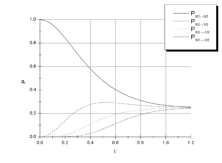
Figure 3: .

Transition probabilities from the state with $s_{z}=3/2$ to any other state as functions of transverse magnetic field.

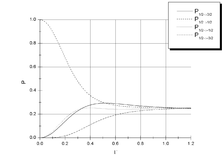
Figure 4: Transition probabilities from the state with $s_{z}=1/2$ to any other state as functions of transverse magnetic field.

In $Fig3$ and $Fig4$ we show the dependences of transition probabilities for $S=3/2$ on $\Gamma$. In adiabatic limit $\Gamma^{2}/\beta>>1$ all states are equally populated after the evolution.

VII Electron motion driven by electric field

.

Now we consider another multi-state Landau-Zener model that, in the absence of the noise, was solved exactly PS . Physically the model describes the transport of a charged particle in a regular linear chain driven by a time-dependent homogeneous external field. Such a model is an idealization of atomic scale molecular wires or linear arrays of quantum dots. An important assumption in the model that makes it exactly solvable is that all sites of the chain are identical and equidistant. External electric field splits the energy levels at different sites of the chain and suppresses the tunnelling between them. Hence the transitions proceed in a narrow time intervals close to moments at which the electric field becomes zero. The noise in such a system arises due to thermal fluctuations chaotically changing the energy of the electron. We suppose that there are no correlations of noise at different sites.

Let us denote $|n\rangle$ a state located at the $n$-th site of the chain. We assume that these states form a complete orthonormal set (Wannier basis). In terms of this set the electron Hamiltonian with linear dependence of an external field on time reads:

$$\hat{H}=\sum\limits_{n}(g\mid n\rangle\langle n+1\mid+c.c.)+nvt\mid n\rangle\langle n\mid+\eta_{n}(t)\mid n\rangle\langle n\mid$$ (55)

where $v$ and $g$ are constants and we assume that the noise power is the same for all sites i.e. $<\eta_{m}\eta_{n}>=2\gamma\delta_{mn}$. The derivation of the master equation for this case is similar to that of the previous section. We consider only the limit of strong noise $\gamma>>g$. Then, as in previous example, the non-diagonal elements of the density matrix $\rho_{i,j}$ with $|i-j|>1$ can be neglected. Equations for diagonal matrix elements of the density matrix are:

$$\dot{\rho_{nn}}=-ig(\rho_{n+1,n}+\rho_{n-1,n}-\rho_{n,n+1}-\rho_{n,n-1})$$ (56)

Equations for non-diagonal elements after the averaging over the random noise read:

$$\begin{array}[]{l}\dot{\rho}_{n+1,n}=(-ivt-2\gamma)\rho_{n+1,n}-ig(\rho_{n,n}-\rho_{n+1,n+1})\\ \dot{\rho}_{n-1,n}=(ivt-2\gamma)\rho_{n-1,n}-ig(\rho_{n,n}-\rho_{n-1,n-1})\end{array}$$ (57)

Neglecting again time derivatives in these equations, we find:

$$\begin{array}[]{l}\rho_{n+1,n}=\frac{-ig}{ivt+2\gamma}(\rho_{n,n}-\rho_{n+1,n+1})\\ \rho_{n-1,n}=\frac{ig}{ivt-2\gamma}(\rho_{n,n}-\rho_{n-1,n-1})\end{array}$$ (58)

Substituting (58) into the equations (56) for diagonal elements, we obtain the evolution equations for diagonal matrix elements of the density matrix $\rho_{n,n}$:

$$\dot{\rho}_{n,n}=g^{2}\left(\frac{1}{ivt-2\gamma}-\frac{1}{ivt+2\gamma}\right)(2\rho_{n,n}-\rho_{n+1,n}-\rho_{n-1,n})$$ (59)

Without loss of generality we can assume that initially, at $t=-\infty$, the particle was located at the site number zero. It can be treated as initial conditions for the master equation: $\rho_{0,0}(t=-\infty)=1$ and all other elements of the density matrix are zeros at $t=-\infty$. Then diagonal matrix elements $\rho_{n,n}$ acquire the meaning of transition probabilities from zeroth to the $n$-th site at a current time $t$. As in the previous example we can find the solution for a chain of arbitrary number of sites in the matrix form.

In the limit of infinite number of sites a compact solution can be found by employing the Fourier-transformation $\rho_{n,n}=\frac{1}{2\pi}\int_{0}^{2\pi}e^{in\phi}u(\phi,t)$. The system of coupled differential equations (59) is diagonalized by this transformation. Corresponding differential equation of the first order for the function $u(\phi,t)$ is readily solved. Its solution with the initial condition $u(\phi,-\infty=1)$ is

$$u(\phi,t)=\exp\left[-2\left(\frac{\pi}{2}+\arctan\frac{vt}{2\gamma}\right)(1-\cos\phi)\right]$$

In the limit $t\rightarrow+\infty$ it approaches its limiting value:

$$u(\phi,t\rightarrow+\infty)=e^{\frac{-4\pi g^{2}}{v}(1-\cos\phi)}$$ (60)

By the inverse Fourier-transformation we find the diagonal elements of the density matrix:

$$\rho_{n,n}(t\rightarrow+\infty)=P_{n}=e^{-\frac{4\pi g^{2}}{v}}I_{n}(\frac{4\pi g^{2}}{v})$$ (61)

Here $P_{n}$ is the transition probability from the site with the index $0$ to the cite with the index $n$ .

It is interesting to compare results of this calculation which incorporates a strong noise with the transition probabilities without noise. In the absence of the noise $(\gamma=0)$ the transition probabilities are PS :

$$P_{n}^{(coh)}=|J_{n}(\sqrt{8\pi}g)|^{2}$$ (62)

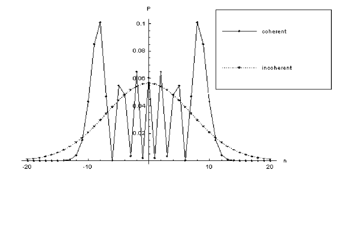
Figure 5: Comparison of transition probabilities in coherent (without noise) and incoherent (with strong noise) LZ models on the chain.

$Fig.5$ shows a typical behavior of the transition probabilities for both cases. The difference in the behavior is clearly pronounced. In the absence of the noise the transition probabilities oscillate as functions of $n$ and $g$ (see PS for details). These oscillations arise due to the interference among the amplitudes of different Feynman paths leading from the initial to the final point. In the case of a strong noise these oscillation are suppressed by the noise imposed decoherence and the probability distribution is a smooth bell-like curve. A simple parameter that is related to the effective diffusion coefficient and can be measured experimentally is the average square displacement of the particle during one sweep of the external field. For a chain with a strong noise it is:

$$<n^{2}>=\sum\limits_{n=-\infty}^{+\infty}n^{2}e^{\frac{-4\pi g^{2}}{v}}I_{n}(\frac{4\pi g^{2}}{v})=\frac{4\pi g^{2}}{v}$$ (63)

Despite a strong difference in the distribution functions, the average square displacement (63) coincides with that for the coherent evolution without noise.

VIII Conclusion

In conclusion, we have derived the formula for the transition probabilities at the non-adiabatic crossing of two levels coupled by a fast non-diagonal random field in the Landau-Zener approximation. Depending on the strength of parameters it interpolates between the Landau-Zener formula for noiseless system and the Kayanuma’s result for transitions mediated by the transverse noise only. We have determined the time intervals during which transitions are substantial and showed that time of transitions mediated by the constant field is much shorter than the time necessary for transition caused by the fast noise. Our numerical simulations are in a good agreement with the analytical formulas . We have discovered an important property of the non-adiabatic tunnelling process: its probability depends not on the ”power” of the noise $\int_{-\infty}^{\infty}g(t)dt$ but rather on the coupling to the noise $g(0)$. The former usually is responsible for the decoherence rate in systems without time- dependent fields. Measurements of the LZ transition probability can provide the information about the value of this coupling. The multi-level systems placed in regular time-dependent fields feel subtle differences of the noise statistical properties.

We assumed that the diagonal noise does not dominate. In this situation it does not play any role. However, if the component of the diagonal noise is much stronger than non-diagonal ones, the situation may change drastically. The problem of strong transverse field compatible with noise inverse correlation time also remains open.

We have extended the formulas and methods employed for two-level systems to a couple of multi-state LZ systems: an arbitrary spin experiencing the time-dependent regular and random magnetic field and a linear chain of sites in the external time-dependent homogeneous electric field plus noise. The Landau-Zener transitions for spins higher than $1/2$ were observed in a number of systems Kaz ; agu ; Suo . Therefore we believe that our solutions can be checked experimentally.

IX acknowledgements

This work was supported by the NSF under the grant DMR0072115 and DMR 0103455, by the TITF of Texas A$\&$M University and by the DOE under the grant DE-FG03-96ER45598. We are grateful to M. Nishino for useful discussion.

References

- (1) V. May, O. Kuhn, ”Charge and Energy Transfer Dynamics in Molecular Systems”, WILEY-VCH Verlag Berlin GmbH (2000)
- (2) D. A. Harmin, P. N. Price, Phys. Rev. A. 49 (1994) 1933
- (3) E.E. Nikitin, S. Ya Umanskii ”Theory of Slow Atomic Collisions”,
- (4) W. Wernsdorfer, R. Sessoli, Science, 284, 133 (1999)
- (5) W. Wernsdorfer, , T. Ohm, C. Sangregorio, R. Sessoli, D.
- (6) R. Giraud, W. Wernsdorfer, A.M.Tkachuk, D. Mailly, B. Barbara, cond-mat/0102231
- (7) E. Kececioglu, A. Garg, Phys.Rev.B 63, 064422 (2001),
- (8) D.A. Garanin, E.M. Chudnovsky Phys.Rev. B 65 094423 (2002)
- (9) N.V. Prokof’ev, P.C.E. Stamp, Phys.Rev.Lett. 80, 5794 (1998)
- (10) D. V. Averin, Phys. Rev. Lett. 82, 3685 (1999)
- (11) D. V. Averin, A. Bardas, Phys. Rev. Lett. 75, 1831 (1995)
- (12) Yu. Gefen, E. Ben-Jacob, A. O. Caldeira, Phys. Rev. B. 36 (1987) 2770-2782
- (13) D. Iliescu, S. Fishman, E. Ben-Jacob, Phys. Rev. B, 46 (1992) 675-685
- (14) F. Renzoni, T. Brandes, Phys. Rev. B 64 (2001) 245301, cond-mat/0109335
- (15) V.A. Yurovsky, A. Ben-Reuven, Phys. Rev. A. V63, 043404 (2001)
- (16) A.V. Shytov, D.A. Ivanov, M.V. Feigel’man cond-mat/0110490
- (17) D. Lubin, Yu. Gefen, I. Goldhirsch, Phys.Rev.B 41, 4441 (1990)
- (18) Yu. N. Demkov, V. I. Osherov, Zh. Exp. Teor. Fiz. 53 (1967) 1589 (Engl. transl. 1968 Sov. Phys.-JETP 26, 916)
- (19) C.E. Carroll, F. T. Hioe, J. Phys. A: Math. Gen. 19, 1151-1161 (1986)
- (20) S. Brundobler, V. Elser, J. Phys. A: Math.Gen. 26 (1993) 1211-1227
- (21) Yu. N. Demkov, V. N. Ostrovsky, J. Phys. B: At. Mol. Opt. Phys. 28 (1995) 403-414
- (22) V.N. Ostrovsky, H. Nakamura, J.Phys A: Math. Gen. 30 6939-6950(1997)
- (23) Y.N. Demkov, V.N. Ostrovsky, J. Phys. B. 34 (12), (2001) 2419-2435
- (24) F.T. Hioe, J. Opt. Soc. Am. B 4, 1237-1332 (1987)
- (25) Y. N. Demkov, V.N. Ostrovsky, Phys. Rev. A 61, 032705 (2000)
- (26) V.L. Pokrovsky, N.A. Sinitsyn, Phys. Rev. B 65, 153105 (2002)
- (27) T. Usuki, Phys.Rev.B 56, 13360 (1997)
- (28) N.A. Sinitsyn, Phys.Rev.B66, 205303 (2002)
- (29) J. Liu, L-B Fu, B-Y. Ou, S-G. Chen, Q. Niu, Phys.Rev. A 66, 023404 (2002), quant-ph/0105140
- (30) J. Liu, B. Wu, L. Fu, R. B. Diener, and Q. Niu, Phys. Rev. B 65, 224401 (2002)
- (31) O. Zobay, B.M. Garraway,Phys. Rev. A 61, 033603 (2000), cond-mat/9908174
- (32) D.A. Garanin, R. Schilling, Phys.Rev. B66, 174438 (2002),cond-mat/0207418
- (33) K. Saito, S. Miyashita, H. De Raedt, Phys. Rev. B, V.60, 21 (1999) 14553
- (34) Y. Kayanuma, J. Phys. Soc. Japan, V53, No.1 (1984) 108
- (35) Y. Kayanuma, H. Nakayama, Phys.Rev. B, V.57, 20 (1998) 13009
- (36) Y. Kayanuma, J. Phys. Soc. Japan, V.54, No.5 (1985) 2037
- (37) M. Nishino, K. Saito, S. Miyashita, Phys. Rev. B 65, 014403 (2002), cond-mat/0103553
- (38) K. Saito, Y. Kayanuma, Phys. Rev. A 65, 033407 (2002), cond-mat/0111420
- (39) P. Ao, J. Rammer, Phys. Rev. B, V.43, 7 (1991) 5397
- (40) H. Kobayashi, N. Hatano, S. Miyashita, Physica A 265 (1999) 565
- (41) E. Shimshoni, A. Stern, Phys. Rev. B 47, 9523 (1993)
- (42) Y. Kayanuma, Phys.Rev. B 47, 9940 (1993)
- (43) M.N. Leuenberger, D. Loss, cond-mat/9911065
- (44) V.G. Benzatand, G. Strini, quant-ph/0203110
- (45) T. Usuki, Phys.Rev.B 57, 7124 (1998)
- (46) A.A. Abrikosov, L.P. Gorkov, I.E. Dzyaloshinskii, ”Methods of Quantum Field Theory in Statistical Physics”, Prentice Hall, New York (1963)
- (47) A.K. Kazansky, V.N. Ostrovsky, J. Phys. B: At. Mol. Opt. Phys. 29 (1996) L855-L861
- (48) A. Aguilar, M. Gonzalez, L.V. Poluyanov, J. Phys.B: At. Mol. Opt. Phys. 33 (2000) 4815
- (49) K-A. Suominen, E. Tiesinga, P.S. Julienne, Phys. Rev. A 58 (1998) 3983
- (50) K. Mullen, D. Ben-Jacob, Yu. Gefen, Z. Schuss, Phys.Rev.Lett. 62, 2543 (1989)
- (51) A.D. Armour, A. MacKinnon, Phys.Rev. B 66, 035333 (2002)