Shot Noise of Cotunneling Current

Abstract

We study the noise of the cotunneling current through one or several tunnel-coupled quantum dots in the Coulomb blockade regime. The various regimes of weak and strong, elastic and inelastic cotunneling are analyzed for quantum-dot systems (QDS) with few-level, nearly-degenerate, and continuous electronic spectra. In the case of weak cotunneling we prove a non-equilibrium fluctuation-dissipation theorem which leads to a universal expression for the noise-to-current ratio (Fano factor). The noise of strong inelastic cotunneling can be super-Poissonian due to switching between QDS states carrying currents of different strengths. The transport through a double-dot (DD) system shows an Aharonov-Bohm effect both in noise and current. In the case of cotunneling through a QDS with a continuous energy spectrum the Fano factor is very close to one.

1 Introduction

In recent years, there has been great interest in the shot noise in mesoscopic systems [1], because it contains additional information about correlations, which is not contained, e.g., in the linear response conductance. The shot noise is characterized by the Fano factor $F=S/eI$, the dimensionless ratio of the zero-frequency noise power $S$ to the average current $I$. While it assumes the Poissonian value $F=1$ in the absence of correlations, it becomes suppressed or enhanced when correlations set in as e.g. imposed by the Pauli principle or due to interaction effects. In the present paper we study the shot noise of the cotunneling [2, 3] current. We consider the transport through a quantum-dot system (QDS) in the Coulomb blockade (CB) regime, in which the quantization of charge on the QDS leads to a suppression of the sequential tunneling current except under certain resonant conditions. We consider the transport away from these resonances and study the next-order contribution to the current  (see Fig. 1). We find that in the weak cotunneling regime, i.e. when the cotunneling rate $I/e$ is small compared to the intrinsic relaxation rate $w_{\rm in}$ of the QDS to its equilibrium state due to the coupling to the environment, $I/e\gg w_{\rm in}$, the zero-frequency noise takes on its Poissonian value, as first obtained for a special case in [6]. This result is generalized here, and we find a universal relation between noise and current for the QDS in the first nonvanishing order in the tunneling perturbation. Because of the universal character of this result Eq. (12) we call it the nonequilibrium fluctuation-dissipation theorem (FDT) [7] in analogy with linear response theory.

One might expect however that the cotunneling, being a two-particle process, may lead to strong correlations in the shot noise and to the deviation of the Fano factor from its Poissonian value $F=1$. We show in Sec. 4 that this is indeed the case for the regime of strong cotunneling, $I/e\gg w_{\rm in}$. Specifically, for a two-level QDS we predict giant (divergent) super-Poissonian noise [8] (see Sec. 5): The QDS goes into an unstable mode where it switches between states 1 and 2 with (generally) different currents. In Sec. 6 we consider the transport through a double-dot (DD) system as an example to illustrate this effect (see Eq. (39) and Fig. 2). The Fano factor turns out to be a periodic function of the magnetic flux through the DD leading to an Aharonov-Bohm effect in the noise [9]. In the case of weak cotunneling we concentrate on the average current through the DD and find that it shows Aharonov-Bohm oscillations, which are a two-particle effect sensitive to spin entanglement.

Finally, in Sec. 7 we discuss the cotunneling through large QDS with a continuum spectrum. In this case the correlations in the cotunneling current described above do not play an essential role. In the regime of low bias, elastic cotunneling dominates transport,[2] and thus the noise is Poissonian. In the opposite case of large bias, the transport is governed by inelastic cotunneling, and in Sec. 7 we study heating effects which are relevant in this regime.

2 Model system

In general, the QDS can contain several dots, which can be coupled by tunnel junctions, the DD being a particular example [6]. The QDS is assumed to be weakly coupled to external metallic leads which are kept at equilibrium with their associated reservoirs at the chemical potentials $\mu_{l}$, $l=1,2$, where the currents $I_{l}$ can be measured and the average current $I$ through the QDS is defined by Eq. (5). Using a standard tunneling Hamiltonian approach [10], we write

$$H=H_{0}+V\,,\quad H_{0}=H_{L}+H_{S}+H_{\rm int}\,,$$ (1)

$$H_{L}=\sum_{l=1,2}\sum_{k}\varepsilon_{k}c_{lk}^{{\dagger}}c_{lk}\,,\quad H_{S}=\sum_{p}\varepsilon_{p}d_{p}^{{\dagger}}d_{p}\,,$$ (2)

$$V=\sum_{l=1,2}(D_{l}+D^{{\dagger}}_{l}),\quad D_{l}=\sum_{k,p}T_{lkp}c_{lk}^{{\dagger}}d_{p}\,,$$ (3)

where the terms $H_{L}$ and $H_{S}$ describe the leads and QDS, respectively (with $k$ and $p$ from a complete set of quantum numbers),and tunneling between leads and QDS is described by the perturbation $V$. The interaction term $H_{\rm int}$ does not need to be specified for our proof of the universality of noise in Sec. 3. The $N$-electron QDS is in the cotunneling regime where there is a finite energy cost $\Delta_{\pm}(l,N)>0$ for the electron tunneling from the Fermi level of the lead $l$ to the QDS ($+$) and vice versa ($-$). This energy cost is of the order of the charging energy $E_{C}$ and much larger than the temperature, $\Delta_{\pm}(l,N)\sim E_{C}\gg k_{B}T$, so that only processes of second order in $V$ are allowed.

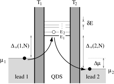
Figure 1: The quantum dot system (QDS) is coupled to two external leads $l=1,2$ via tunneling barriers. The tunneling between the QDS and the leads is parametrized by the tunneling amplitudes $T_{l}$, where the lead and QDS quantum numbers $k$ and $p$ have been dropped for simplicity, see Eq. (3). The leads are at the chemical potentials $\mu_{1,2}$, with an applied bias $\Delta\mu=\mu_{1}-\mu_{2}$. The eigenstates of the QDS with one added electron ($N+1$ electrons in total) are indicated by their energies $E_{1}$, $E_{2}$, etc., with average level-spacing $\delta E$. In the cotunneling regime there is a finite energy cost $\Delta_{\pm}(l,N)>0$ for the electron tunneling from the Fermi level of the lead $l$ to the QDS ($+$) and vice versa ($-$), so that only processes of second order in $V$ (visualized by two arrows) are allowed.

To describe the transport through the QDS we apply standard methods [10] and adiabatically switch on the perturbation $V$ in the distant past, $t=t_{0}\to-\infty$. The perturbed state of the system is described by the time-dependent density matrix $\rho(t)=e^{-iH(t-t_{0})}\rho_{0}e^{iH(t-t_{0})}$, with $\rho_{0}$ being the grand canonical density matrix of the unperturbed system, $\rho_{0}=Z^{-1}e^{-K/k_{B}T}$, where we set $K=H_{0}-\sum_{l}\mu_{l}N_{l}$. Because of tunneling the total number of electrons in each lead $N_{l}=\sum_{k}c_{lk}^{{\dagger}}c_{lk}$ is no longer conserved. For the outgoing currents $\hat{I}_{l}=e\dot{N}_{l}$ we have

$$\hat{I}_{l}=ei\left[V,N_{l}\right]=ei(D^{{\dagger}}_{l}-D_{l})\,.$$ (4)

The observables of interest are the average current $I\equiv I_{2}=-I_{1}$ through the QDS, and the spectral density of the noise $S_{ll^{\prime}}(\omega)=\int dtS_{ll^{\prime}}(t)\exp(i\omega t)$,

$$I_{l}={\rm Tr}\rho(0)\hat{I}_{l},\quad S_{ll^{\prime}}(t)={\rm Re}\,{\rm Tr}\,\rho(0)\delta I_{l}(t)\delta I_{l^{\prime}}(0)\,,$$ (5)

where $\delta I_{l}=\hat{I}_{l}-I_{l}$. Below we will use the interaction representation where Eq. (5) can be rewritten by replacing $\rho(0)\to\rho_{0}$ and $\hat{I}_{l}(t)\to U^{{\dagger}}(t)\hat{I}_{l}(t)U(t)$, with

$$U(t)=T\exp\left[-i\int^{t}_{-\infty}dt^{\prime}\,V(t^{\prime})\right]\,.$$ (6)

In this representation, the time dependence of all operators is governed by the unperturbed Hamiltonian $H_{0}$.

3 Weak cotunneling: Non-equilibrium fluctuation-dissipation
theorem

In this section we prove the universality of noise of tunnel junctions in the weak cotunneling regime $I/e\ll w_{\rm in}$ keeping the first nonvanishing order in the tunneling Hamiltonian $V$. Since our final result (12) can be applied to quite general systems out-of-equilibrium we call this result the non-equilibrium fluctuation-dissipation theorem (FDT). In particular, the geometry of the QDS and the interaction $H_{\rm int}$ are completely arbitrary for the discussion of the non-equilibrium FDT in this section.

We note that the two currents $\hat{I}_{l}$ are not independent, because $[\hat{I}_{1},\hat{I}_{2}]\neq 0$, and thus all correlators $S_{ll^{\prime}}$ are nontrivial. The charge accumulation on the QDS for a time of order $\Delta_{\pm}^{-1}$ leads to an additional contribution to the noise at finite frequency $\omega$. Thus, we expect that for $\omega\sim\Delta_{\pm}$ the correlators $S_{ll^{\prime}}$ cannot be expressed through the steady-state current $I$ only and thus $I$ has to be complemented by some other dissipative counterparts, such as differential conductances $G_{ll^{\prime}}$. On the other hand, at low enough frequency, $\omega\ll\Delta_{\pm}$, the charge conservation on the QDS requires $\delta I_{s}=(\delta I_{2}+\delta I_{1})/2\approx 0$. Below we concentrate on the limit of low frequency and neglect contributions of order of $\omega/\Delta_{\pm}$ to the noise power. In the Appendix we prove that $S_{ss}\sim(\omega/\Delta_{\pm})^{2}$ (see Eq. (67)), and this allows us to redefine the current and the noise power as $I\equiv I_{d}=(I_{2}-I_{1})/2$ and $S(\omega)\equiv S_{dd}(\omega)$.  In addition we require that the QDS is in the cotunneling regime, i.e. the temperature is low enough, $k_{B}T\ll\Delta_{\pm}$, although the bias $\Delta\mu$ is arbitrary as soon as the sequential tunneling to the dot is forbidden, $\Delta_{\pm}>0$. In this limit the current through a QDS arises due to the direct hopping of an electron from one lead to another (through a virtual state on the dot) with an amplitude which depends on the energy cost $\Delta_{\pm}$ of a virtual state. Although this process can change the state of the QDS (inelastic cotunneling), the fast energy relaxation in the weak cotunneling regime, $w_{\rm in}\gg I/e$, immediately returns it to the equilibrium state (for the opposite case, see Sec. 4). This allows us to apply a perturbation expansion with respect to tunneling $V$ and to keep only first nonvanishing contributions, which we do next.

It is convenient to introduce the notation $\bar{D}_{l}(t)\equiv\int_{-\infty}^{t}dt^{\prime}\,D_{l}(t^{\prime})$. We notice that all relevant matrix elements, $\langle N|D_{l}(t)|N+1\rangle\sim e^{-i\Delta_{+}t}$, $\langle N-1|D_{l}(t)|N\rangle\sim e^{i\Delta_{-}t}$, are fast oscillating functions of time. Thus, under the above conditions we can write $\bar{D}_{l}(\infty)=0$, and even more general, $\int_{-\infty}^{+\infty}dt\,D_{l}(t)e^{\pm i\omega t}=0$ (note that we have assumed earlier that $\omega\ll\Delta_{\pm}$). Using these equalities and the cyclic property of the trace we obtain the following results (for details of the derivation, see Appendix A),

$$I=e\int\limits_{-\infty}^{\infty}dt\,\langle[A^{{\dagger}}(t),A(0)]\rangle,\qquad A=D_{2}\bar{D}^{{\dagger}}_{1}+D^{{\dagger}}_{1}\bar{D}_{2}\,,$$ (7)

$$S(\omega)=e^{2}\int\limits^{\infty}_{-\infty}dt\,\cos(\omega t)\langle\{A^{{\dagger}}(t),A(0)\}\rangle\,,$$ (8)

where we have dropped a small contribution of order $\omega/\Delta_{\pm}$ and used the notation $\langle\ldots\rangle={\rm Tr}\rho_{0}(\ldots)$.

Next we apply the spectral decomposition to the correlators Eqs. (7) and (8), a similar procedure to that which also leads to the equilibrium fluctuation-dissipation theorem. The crucial observation is that $[H_{0},N_{l}]=0$, $l=1,2$. Therefore, we are allowed to use for our spectral decomposition the basis $|{\bf n}\rangle=|E_{{\bf n}},N_{1},N_{2}\rangle$ of eigenstates of the operator $K=H_{0}-\sum_{l}\mu_{l}N_{l}$, which also diagonalizes the grand-canonical density matrix $\rho_{0}$, $\rho_{{\bf n}}=\langle{\bf n}|\rho_{0}|{\bf n}\rangle=Z^{-1}\exp[-E_{{\bf n}}/k_{B}T]$. We introduce the spectral function,

$${\cal A}(\omega)=2\pi\sum_{{\bf n},{\bf m}}(\rho_{{\bf n}}+\rho_{{\bf m}})|\langle{\bf m}|A|{\bf n}\rangle|^{2}\delta(\omega+E_{{\bf n}}-E_{{\bf m}})\,,$$ (9)

and rewrite Eqs. (7) and (8) in the matrix form in the basis $|{\bf n}\rangle$ taking into account that the operator $A$, which plays the role of the effective cotunneling amplitude, creates (annihilates) an electron in the lead 2 (1) (see Eqs. (3) and (7)). We obtain following expressions

$$I(\Delta\mu)=e\tanh\left[\frac{\Delta\mu}{2k_{B}T}\right]{\cal A}(\Delta\mu)\,,$$ (10)

$$S(\omega,\Delta\mu)=\frac{e^{2}}{2}\sum_{\pm}{\cal A}(\Delta\mu\pm\omega)\,.$$ (11)

We note that because of additional integration over time $t$ in the amplitude $A$ (see Eq. (7)), the spectral density ${\cal A}$ depends on $\mu_{1}$ and $\mu_{2}$ separately. However, away from the resonances, $\omega\ll\Delta_{\pm}$, only $\Delta\mu$-dependence is essential, and thus ${\cal A}$ can be regarded as being one-parameter function.  Comparing Eqs. (10) and (11), we obtain

$$S(\omega,\Delta\mu)=\frac{e}{2}\sum_{\pm}\coth\left[\frac{\Delta\mu\pm\omega}{2k_{B}T}\right]I(\Delta\mu\pm\omega)$$ (12)

up to small terms on the order of $\omega/\Delta_{\pm}$. This equation represents our nonequilibrium FDT for the transport through a QDS in the weak cotunneling regime. A special case with $T,\omega=0$, giving $S=eI$, has been derived earlier [6]. To conclude this section we would like to list again the conditions used in the derivation. The universality of noise to current relation Eq. (12) proven here is valid in the regime in which it is sufficient to keep the first nonvanishing order in the tunneling $V$ which contributes to transport and noise. This means that the QDS is in the weak cotunneling regime with $\omega,k_{B}T\ll\Delta_{\pm}$, and $I/e\ll w_{\rm in}$.

4 Strong cotunneling: Correlation correction to noise

In this section we consider the QDS in the strong cotunneling regime, $w_{\rm in}\ll I/e$. Under this assumption the intrinsic relaxation in the QDS is very slow and will in fact be neglected. Thermal equilibration can only take place via coupling to the leads (see Sec. 7). Due to this slow relaxation in the QDS we find that there are non-Poissonian correlations $\Delta S$ in the current through the QDS because the QDS has a “memory”; the state of the QDS after the transmission of one electron influences the transmission of the next electron. The microscopic theory of strong cotunneling has been developed in Ref. [5] based on the density-operator formalism and using the projection operator technique. Here we discuss the assumptions and present the results of the theory, equations (14), (15), and (17-19), which are the basis for our further analysis in the Secs. 5 and 6.

First, we assume that the system and bath are coupled only weakly and only via the perturbation $V$, Eq. (3). The interaction part $H_{\rm int}$ of the unperturbed Hamiltonian $H_{0}$, Eq. (1), must therefore be separable into a QDS and a lead part, $H_{\rm int}=H_{S}^{\rm int}+H_{L}^{\rm int}$. Moreover, $H_{0}$ conserves the number of electrons in the leads, $[H_{0},N_{l}]=0$, where $N_{l}=\sum_{k}c_{lk}^{\dagger}c_{lk}$. The assumption of weak coupling allows us to keep only the second-order in $V$ contributions to the “golden rule” rates (15) for the Master equation (14).

Second, we assume that in the distant past, $t_{0}\rightarrow-\infty$, the system is in an equilibrium state

$$\rho_{0}=\rho_{S}\otimes\rho_{L},\quad\rho_{L}=\frac{1}{Z_{L}}e^{-K_{L}/k_{B}T},$$ (13)

where $Z_{L}={\rm Tr}\,\exp[-K_{L}/k_{B}T]$, $K_{L}=H_{L}-\sum_{l}\mu_{l}N_{l}$, and $\mu_{l}$ is the chemical potential of lead $l$. Note that both leads are kept at the same temperature $T$. Physically, the product form of $\rho_{0}$ in Eq. (13) describes the absence of correlations between the QDS and the leads in the initial state at $t_{0}$. Furthermore, we assume that the initial state $\rho_{0}$ is diagonal in the eigenbasis of $H_{0}$, i.e. that the initial state is an incoherent mixture of eigenstates of the free Hamiltonian.

Finally, we consider the low-frequency noise, $\omega\ll\Delta_{\pm}$, i.e. we neglect the accumulation of the charge on the QDS (in the same way as in the Sec. 3). Thus we can write $S_{ll}(\omega)=-S_{l\neq l^{\prime}}(\omega)\equiv S(\omega)$. This restriction will be lifted in the end of the Sec. 6.1.

We note that the above assumptions limit the generality of the results of present section as compared to those of Sec. 3. On the other hand, they allow us to reduce the problem of the noise calculations to the solution of the Master equation

$$\dot{\rho}_{n}(t)=\sum_{m}\left[w_{nm}\rho_{m}(t)-w_{mn}\rho_{n}(t)\right],$$ (14)

with the stationary state condition $\sum_{m}(w_{nm}\bar{\rho}_{m}-w_{mn}\bar{\rho}_{n})=0$. This “classical” master equation describes the dynamics of the QDS, i.e. it describes the rates with which the probabilities $\rho_{n}$ for the QDS being in state $|n\rangle$ change. The rates $w_{nm}=\sum_{l,l^{\prime}=1,2}w_{nm}(l^{\prime},l)$ are the sums of second-order “golden rule” rates

$$w_{nm}(l^{\prime},l)=2\pi\sum_{\bar{m},\bar{n}}|\langle{\bf n}|(D^{\dagger}_{l},D_{l^{\prime}})|{\bf m}\rangle|^{2}\delta(E_{\bf m}-E_{\bf n}-\Delta\mu_{ll^{\prime}})\rho_{L,\bar{m}}.$$ (15)

for all possible cotunneling transitions from lead $l$ to lead $l^{\prime}$. In the last expression, $\Delta\mu_{ll^{\prime}}=\mu_{l}-\mu_{l^{\prime}}$ denotes the chemical potential drop between lead $l$ and lead $l^{\prime}$, and $\rho_{L,\bar{m}}=\langle\bar{m}|\rho_{L}|\bar{m}\rangle$. We have defined the second order hopping operator

$$(D^{\dagger}_{l},D_{l^{\prime}})=D_{l^{\prime}}\bar{D}^{\dagger}_{l}+D^{\dagger}_{l}\bar{D}_{l^{\prime}},$$ (16)

where $D_{l}$ is given in Eq. (3), and $\bar{D_{l}}=\int_{-\infty}^{0}D_{l}(t)dt$. Note, that $(D^{\dagger}_{l},D_{l^{\prime}})$ is the amplitude of cotunneling from the lead $l$ to the lead $l^{\prime}$ (in particular, we can write $A=(D^{\dagger}_{1},D_{2})$, see Eq. (7)). The combined index ${\bf m}=(m,\bar{m})$ contains both the QDS index $m$ and the lead index $\bar{m}$. Correspondingly, the basis states used above are $|{\bf m}\rangle=|m\rangle|\bar{m}\rangle$ with energy $E_{\bf m}=E_{m}+E_{\bar{m}}$, where $|m\rangle$ is an eigenstate of $H_{S}+H_{S}^{\rm int}$ with energy $E_{m}$, and $|\bar{m}\rangle$ is an eigenstate of $H_{L}+H_{L}^{\rm int}-\sum_{l}\mu_{l}N_{l}$ with energy $E_{\bar{m}}$.

For the average current $I$ and the noise power $S(\omega)$ we obtain [5]

$$I = e\sum_{mn}w^{I}_{nm}\bar{\rho}_{m},\quad w^{I}_{nm}=w_{nm}(2,1)-w_{nm}(1,2),$$ (17)

$$S(\omega) = e^{2}\sum_{mn}[w_{nm}(2,1)+w_{nm}(1,2)]\bar{\rho}_{m}+\Delta S(\omega),$$ (18)

$$\Delta S(\omega) = e^{2}\!\!\!\!\!\!\sum_{n,m,n^{\prime},m^{\prime}}w^{I}_{nm}\delta\rho_{mn^{\prime}}(\omega)w^{I}_{n^{\prime}m^{\prime}}\bar{\rho}_{m^{\prime}},$$ (19)

where $\delta\rho_{nm}(\omega)=\rho_{nm}(\omega)-2\pi\delta(\omega)\bar{\rho}_{n}$, and $\bar{\rho}_{n}$ is the stationary density matrix. Here, $\rho_{nm}(\omega)$ is the Fourier-transformed conditional density matrix, which is obtained from the symmetrized solution $\rho_{n}(t)=\rho_{n}(-t)$ of the master equation Eq. (14) with the initial condition $\rho_{n}(0)=\delta_{nm}$.

An explicit result for the noise in this case can be obtained by making further assumptions about the QDS and the coupling to the leads, see the following sections. For the general case, we only estimate $\Delta S$. The current is of the order $I\sim ew$, with $w$ some typical value of the cotunneling rate $w_{nm}$, and thus $\delta I\sim ew$. The time between switching from one dot-state to another due to cotunneling is approximately $\tau\sim w^{-1}$. The correction $\Delta S$ to the Poissonian noise can be estimated as $\Delta S\sim\delta I^{2}\tau\sim e^{2}w$, which is of the same order as the Poissonian contribution $eI\sim e^{2}w$. Thus the correction to the Fano factor is of order unity. (Note however, that under certain conditions the Fano factor can diverge, see Secs. 5 and 6.) In contrast to this, we find that for elastic cotunneling the off-diagonal rates vanish, $w_{nm}\propto\delta_{nm}$, and therefore $\delta\rho_{nn}=0$ and $\Delta S=0$. Moreover, at zero temperature, either $w_{nn}(2,1)$ or $w_{nn}(1,2)$ must be zero (depending on the sign of the bias $\Delta\mu$). As a consequence, for elastic cotunneling we find Poissonian noise, $F=S(0)/e|I|=1$.

5 Cotunneling through nearly degenerate states

Suppose the QDS has nearly degenerate states with energies $E_{n}$, and level spacing $\delta\!E_{nm}=E_{n}-E_{m}$, which is much smaller than the average level spacing $\delta E$. In the regime, $\Delta\mu,k_{B}T,\delta\!E_{nm}\ll\delta E$, the only allowed cotunneling processes are the transitions between nearly degenerate states. The noise power is given by Eqs. (18) and (19), and below we calculate the correlation correction to the noise, $\Delta S$. To proceed with our calculation we rewrite Eq. (14) for $\delta\rho(t)$ as a second-order differential equation in matrix form

$$\delta\ddot{\rho}(t)=W^{2}\delta\rho(t),\quad\delta\rho(0)=1-\bar{\rho},$$ (20)

where $W$ is defined as $W_{nm}=w_{nm}-\delta_{nm}\sum_{m^{\prime}}w_{m^{\prime}n}$. We solve this equation by Fourier transformation,

$$\delta\rho(\omega)=-\frac{2W}{W^{2}+\omega^{2}1},$$ (21)

where we have used $W\bar{\rho}=0$. We substitute $\delta\rho$ from this equation into Eq. (19) and write the result in a compact matrix form,

$$\Delta S(\omega)=-e^{2}\sum_{n,m}\left[w^{I}\frac{2W}{W^{2}+\omega^{2}1}w^{I}\bar{\rho}\right]_{nm}.$$ (22)

This equation gives the formal solution of the noise problem for nearly degenerate states. As an example we consider a two-level system.

Using the detailed balance equation, $w_{21}\rho_{1}=w_{12}\rho_{2}$, we obtain for the stationary probabilities $\rho_{1}=w_{12}/(w_{12}+w_{21})$, and $\rho_{2}=w_{21}/(w_{12}+w_{21})$. From Eq. (17) we get

$$I=e\frac{w_{12}(w^{I}_{11}+w^{I}_{21})+w_{21}(w^{I}_{22}+w^{I}_{12})}{w_{12}+w_{21}}.$$ (23)

A straightforward calculation with the help of Eq. (21) gives for the correction to the Poissonian noise

$$\Delta S(\omega) = \frac{2e^{2}(w^{I}_{11}+w^{I}_{21}-w^{I}_{22}-w^{I}_{12})}{(w_{12}+w_{21})[\omega^{2}+(w_{12}+w_{21})^{2}]}\times$$ (24)

$$\times \left[w^{I}_{11}w_{12}w_{21}+w^{I}_{12}w^{2}_{21}-(1\leftrightarrow 2)\right].$$

In particular, the zero frequency noise $\Delta S(0)$ diverges if the “off-diagonal” rates $w_{nm}$ vanish. This divergence has to be cut at $\omega$, or at the relaxation rate $w_{\rm in}$ due to coupling to the bath (since $w_{12}$ in this case has to be replaced with $w_{12}+w_{\rm in}$). The physical origin of the divergence is rather transparent: If the off-diagonal rates $w_{12},w_{21}$ are small, the QDS goes into an unstable state where it switches between states 1 and 2 with different currents in general [12]. The longer the QDS stays in the state 1 or 2 the larger the zero-frequency noise power is. However, if $w^{I}_{11}+w^{I}_{21}=w^{I}_{22}+w^{I}_{12}$, then $\Delta S(\omega)$ is suppressed to 0. For instance, for the QDS in the spin-degenerate state with an odd number of electrons $\Delta S(\omega)=0$, since the two states $|\uparrow\rangle$ and $|\downarrow\rangle$ are physically equivalent. The other example of such a suppression of the correlation correction $\Delta S$ to noise is given by a multi-level QDS, $\delta E\ll E_{C}$, where the off-diagonal rates are small compared to the diagonal (elastic) rates [2]. Indeed, since the main contribution to the elastic rates comes from transitions through many virtual states, which do not participate in inelastic cotunneling, they do not depend on the initial conditions, $w^{I}_{11}=w^{I}_{22}$, and cancel in the numerator of Eq. (24), while they are still present in the current. Thus the correction $\Delta S/I$ vanishes in this case. Further below in this section we consider a few-level QDS, $\delta E\sim E_{C}$, where $\Delta S\neq 0$.

To simplify further analysis we consider for a moment the case, where the singularity in the noise is most pronounced, namely, $\omega=0$ and $|\delta\!E_{12}|\ll\Delta\mu,k_{B}T$, so that $w^{I}_{12}=w^{I}_{21}$, and $w_{12}=w_{21}$. Then, from Eqs. (23) and (24) we obtain

$$I=\frac{1}{2}(I_{1}+I_{2})\,,\quad I_{n}=e\sum_{m=1,2}w^{I}_{mn}\,,$$ (25)

$$\Delta S(0)=\frac{(I_{1}-I_{2})^{2}}{4w_{12}}\,,$$ (26)

where $I_{n}$ is the current through the $n$-th level of the QDS. Thus in case $|\delta\!E_{12}|\ll\Delta\mu,k_{B}T$ the following regimes have to be distinguished: (1) If $k_{B}T\lesssim\Delta\mu$, then $I_{n}\propto\Delta\mu$, $w_{12}\propto\Delta\mu$, and thus both, the total current $I=e^{-1}G_{D}\Delta\mu$, and the total noise $S=FG_{D}\Delta\mu$ are linear in the bias $\Delta\mu$ (here $G_{D}$ is the conductance of the QDS). The total shot noise in this regime is super-Poissonian with the Fano factor $F\sim I/(ew_{12})\gg 1$. (2) In the regime $\Delta\mu\lesssim k_{B}T\lesssim F^{1/2}\Delta\mu$ the noise correction (26) arises because of the thermal switching the QDS between two states $n=1,2$, where the currents are linear in the bias, $I_{n}\sim G_{D}\Delta\mu/e$. The rate of switching is $w_{12}\propto k_{B}T$, and thus $\Delta S\sim FG_{D}\Delta\mu^{2}/(k_{B}T)$. Since $k_{B}T/\Delta\mu\lesssim F^{1/2}$, the noise correction $\Delta S$ is the dominant contribution to the noise, and thus the total noise $S$ can be interpreted as being a thermal telegraph noise [13]. (3) Finally, in the regime $F^{1/2}\Delta\mu\lesssim k_{B}T$ the first term on the rhs of Eq. (18) is the dominant contribution, and the total noise becomes an equilibrium Nyquist noise, $S=2G_{D}k_{B}T$.

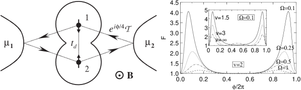
Figure 2: Left: Double-dot (DD) system containing two electrons and being weakly coupled to metallic leads 1, 2, each of which is at the chemical potential $\mu_{1}$, $\mu_{2}$. The tunneling amplitudes between dots and leads are denoted by $\cal T$. The tunneling ($t_{d}$) between the dots results in a singlet-triplet splitting $J\sim t_{d}^{2}/U$ with the singlet being a ground state. The tunneling path between dots and leads 1 and 2 forms a closed loop (shown by arrows) so that the Aharonov-Bohm phase $\phi$ will be accumulated by an electron traversing the DD. Right: The Fano factor $F=S(\omega)/I$, with the noise power $S(\omega)$ given in Eqs. (18) and (39), is plotted as a function of the Aharonov-Bohm phase $\phi$ for the normalized bias $v\equiv\Delta\mu/J=2$ and for four different normalized frequencies $\Omega\equiv\omega/[G(2\Delta\mu-J)]=0.1$, $0.25$, $0.5$, and $1$. Inset: the same, but with fixed frequency $\Omega=0.1$, where the bias $v$ takes the values $1.5$, $3$, and $\infty$.

6 Noise of double-dot system: Two-particle Aharonov-Bohm effect

We notice that for the noise power to be divergent the off-diagonal rates $w_{12}$ and $w_{21}$ have to vanish simultaneously. However, the matrix $w_{nm}$ is not symmetric since the off-diagonal rates depend on the bias in a different way. On the other hand, both rates contain the same matrix element of the cotunneling amplitude $(D^{{\dagger}}_{l},D_{l^{\prime}})$, see Eqs. (15) and (16). Although in general this matrix element is not small, it can vanish because of different symmetries of the two states. To illustrate this effect we consider the transport through a double-dot (DD) system (see Ref. [6] for details) as an example. Two leads are equally coupled to two dots in such a way that a closed loop is formed, and the dots are also connected, see Fig. 2. Thus, in a magnetic field the tunneling is described by the Hamiltonian Eq. (3) with

$$D_{l}=\sum_{s,j}T_{lj}c^{{\dagger}}_{ls}d_{js}\,,\qquad l,j=1,2\,,$$ (27)

$$T_{11}=T_{22}=T^{*}_{12}=T^{*}_{21}=e^{i\phi/4}{\cal T}\,,$$ (28)

where the last equation expresses the equal coupling of dots and leads and $\phi$ is the Aharonov-Bohm phase. Each dot contains one electron, and weak tunneling $t_{d}$ between the dots causes the exchange splitting [14] $J\sim t_{d}^{2}/U$ (with $U$ being the on-site repulsion) between one spin singlet and three triplets

$$|S\rangle=\frac{1}{\sqrt{2}}[d^{{\dagger}}_{1\uparrow}d^{{\dagger}}_{2\downarrow}\!-d^{{\dagger}}_{1\downarrow}d^{{\dagger}}_{2\uparrow}]|0\rangle\,,$$

$$|T_{0}\rangle=\frac{1}{\sqrt{2}}[d^{{\dagger}}_{1\uparrow}d^{{\dagger}}_{2\downarrow}\!+d^{{\dagger}}_{1\downarrow}d^{{\dagger}}_{2\uparrow}]|0\rangle\,,$$ (29)

$$|T_{+}\rangle=d^{{\dagger}}_{1\uparrow}d^{{\dagger}}_{2\uparrow}|0\rangle\,,\quad|T_{-}\rangle=d^{{\dagger}}_{1\downarrow}d^{{\dagger}}_{2\downarrow}|0\rangle\,.$$

In the case of zero magnetic field, $\phi=0$, the tunneling Hamiltonian $V$ is symmetric with respect to the exchange of electrons, $1\leftrightarrow 2$. Thus the matrix element of the cotunneling transition between the singlet and three triplets $\langle S|V(E-H_{0})^{-1}V|T_{i}\rangle$, $i=0,\pm$, vanishes because these states have different orbital symmetries. A weak magnetic field breaks the symmetry, contributes to the off-diagonal rates, and thereby reduces noise. Next, we consider weak and strong cotunneling regimes.

6.1 Weak cotunneling

In this regime, $I/e\ll w_{\rm in}$, according to the non-equilibrium FDT (see Sec. 3) the zero-frequency noise contains the same information as the average current (the Fano factor $F=1$). Therefore, we first concentrate on current. We focus on the regime, $\Delta\mu\gg J$, where inelastic cotunneling [15] occurs with singlet and triplet contributions being different, and where we can neglect the dynamics generated by $J$ compared to the one generated by the bias (”slow spins”). Close to the sequential tunneling peak, $\Delta_{-}\ll\Delta_{+}\sim U$, we keep only the term $D^{{\dagger}}_{1}\bar{D}_{2}$ in the amplitude (7). After some calculations we obtain

$$I=e^{-1}C(\varphi)G\Delta\mu,$$ (30)

$$C(\varphi)=\sum_{s,s^{\prime}}\left[\langle d^{{\dagger}}_{1s^{\prime}}d_{1s}d^{{\dagger}}_{1s}d_{1s^{\prime}}\rangle+\cos\varphi\langle d^{{\dagger}}_{1s^{\prime}}d_{1s}d^{{\dagger}}_{2s}d_{2s^{\prime}}\rangle\right],$$ (31)

where $G=\pi(e\nu{\cal T}^{2}/\Delta_{-})^{2}$ is the conductance of a single dot in the cotunneling regime [16], and we assumed Fermi liquid leads with the tunneling density of states $\nu$. Eq. (30) shows that the cotunneling current depends on the properties of the equilibrium state of the DD through the coherence factor $C(\varphi)$ given in (31). The first term in $C$ is the contribution from the topologically trivial tunneling path (phase-incoherent part) which runs from lead 1 through, say, dot 1 to lead 2 and back. The second term (phase-coherent part) in $C$ results from an exchange process of electron 1 with electron 2 via the leads 1 and 2 such that a closed loop is formed enclosing an area $A$ (see Fig. 2). Note that for singlet and triplets the initial and final spin states are the same after such an exchange process. Thus, in the presence of a magnetic field $B$, an Aharonov-Bohm phase factor $\varphi=ABe/h$ is acquired.

Next, we evaluate $C(\varphi)$ explicitly in the singlet-triplet basis (29) and discuss the applications to the physics of quantum entanglement (see the Ref. [6]). Note that only the singlet $|S\rangle$ and the triplet $|T_{0}\rangle$ are entangled EPR pairs while the remaining triplets are not (they factorize). Assuming that the DD is in one of these states we obtain the important result

$$C(\varphi)=2\mp\cos\varphi\,\,.$$ (32)

Thus, we see that the singlet (upper sign) and the triplets (lower sign) contribute with opposite sign to the phase-coherent part of the current. One has to distinguish, however, carefully the entangled from the non-entangled states. The phase-coherent part of the entangled states is a genuine two-particle effect, while the one of the product states cannot be distinguished from a phase-coherent single-particle effect. Indeed, this follows from the observation that the phase-coherent part in $C$ factorizes for the product states $T_{\pm}$ while it does not so for $S,T_{0}$. Also, for states such as $|\uparrow\downarrow\rangle$ the coherent part of $C$ vanishes, showing that two different (and fixed) spin states cannot lead to a phase-coherent contribution since we know which electron goes which part of the loop.

Finally, we present our results [6] for the high-frequency noise in the quantum range of frequancies, $\omega\sim\Delta_{-}\ll\Delta_{+}$, and in the slow-spin regime $\Delta\mu\gg J$. This range of frequancies is beyond the regime of the applicability of the non-equilibrium FDT, and therefore there is no simple relation between the average current and the noise (see the Sec. 3). After lengthy calculations using the perturbation expansion of (6) up to third order in $V$ we obtain

$$S(\omega)=(e\pi\nu{\cal T}^{2})^{2}\left[X_{\omega}+X^{*}_{-\omega}\right],$$

$$ImX_{\omega}={{C(\varphi)}\over{2\omega}}\left[\theta(\mu_{1}-\omega)-\theta(\mu_{2}-\omega)\right],$$ (33)

$$ReX_{\omega}={{C(\varphi)}\over{2\pi\omega}}sign(\mu_{1}-\mu_{2}+\omega)\ln|{{(\mu_{1}+\omega)(\mu_{2}-\omega)}\over{\mu_{1}\mu_{2}}}|$$

$$-{1\over{2\pi\omega}}\left[\theta(\omega-\mu_{1})\ln|{{\mu_{2}-\omega}\over{\mu_{2}}}|+\theta(\omega-\mu_{2})\ln|{{\mu_{1}-\omega}\over{\mu_{1}}}|\right],$$ (34)

where $\mu_{l}=\Delta_{-}(l)$. Thus the real part of $S(\omega)$ is even in $\omega$, while the imaginary part is odd. A remarkable feature here is that the noise acquires an imaginary (i.e. odd-frequency) part for finite frequencies, in contrast to single-barrier junctions, where Im$S(\omega)$ always vanishes since we have $\delta I_{1}=-\delta I_{2}$ for all times. In double-barrier junctions considered here we find that at small enough bias $\Delta\mu\ll\Delta_{-}=\left(\Delta_{-}(1)+\Delta_{-}(2)\right)/2$, the odd part, Im$S(\omega)$, given in (6.1) exhibits two narrow peaks at $\omega=\pm\mu$, which in real time lead to slowly decaying oscillations,

$$S_{odd}(t)=\pi(e\nu{\cal T}^{2})^{2}C(\varphi)\frac{\sin(\Delta\mu t/2)}{t\Delta_{-}}\sin(t\Delta_{-}).$$ (35)

These oscillations again depend on the phase-coherence factor $C$ with the same properties as discussed before. These oscillations can be interpreted as a temporary build-up of a charge-imbalance on the DD during an uncertainty time $\sim 1/\Delta_{-}$, which results from cotunneling of electrons and an associated time delay between out- and ingoing currents.

6.2 Strong cotunneling

The fact that in the perturbation $V$ all spin indices are traced out helps us to map the four-level system to only two states $|S\rangle$ and $|T\rangle$ classified according to the orbital symmetry (since all triplets are antisymmetric in orbital space). In Appendix B we derive the mapping to a two-level system and calculate the transition rates $w_{nm}(l^{\prime},l)$ ($n,m=1$ for a singlet and $n,m=2$ for all triplets) using Eqs. (15) and (16) with the operators $D_{l}$ given by Eq. (27). Doing this we obtain the following result

$$w_{nm}(1,1)=w_{nm}(2,2)=w_{nm}(1,2)=0,$$

$$w_{nm}=w^{I}_{nm}=\frac{\pi}{2}\left(\frac{\nu{\cal T}^{2}}{\Delta_{-}}\right)^{2}$$

$$\times\left\{\begin{array}[]{ll}(1\!+\!\cos\phi)\Delta\mu&(1\!-\!\cos\phi)(\Delta\mu\!+\!J)\\ 3(1\!-\!\cos\phi)(\Delta\mu\!-\!J)&3(1\!+\!\cos\phi)\Delta\mu\\ \end{array}\right\},$$ (38)

which holds close to the sequential tunneling peak, $\Delta_{-}\ll\Delta_{+}\sim U$ (but still $\Delta_{-}\gg J,\Delta\mu$), and for $\Delta\mu>J$. We substitute this equation into the Eq. (24) and write the correction $\Delta S(\omega)$ to the Poissonian noise as a function of normalized bias $v=\Delta\mu/J$ and normalized frequency $\Omega=e\omega/[G(2\Delta\mu-J)]$

$$\Delta S(\omega)=6eGJ\frac{(v^{2}-1)[1+(v-1)\cos\phi]^{2}(1-\cos\phi)}{(2v-1)^{3}[\Omega^{2}+(1-\cos\phi)^{2}]}.$$ (39)

From this equation it follows that the noise power has singularities as a function of $\omega$ for zero magnetic field, and it has singularities at $\phi=2\pi m$ (where $m$ is integer) as a function of the magnetic field (see Fig. 2). We would like to emphasize that the noise is singular even if the exchange between the dots is weak, $J\ll\Delta\mu$. In the case $\Delta\mu<J$ the transition from the singlet to the triplet is forbidden by conservation of energy, $w_{21}(2,1)=0$, and we immediately obtain from Eq. (24) that $\Delta S(\omega)=0$, i.e. the total noise is Poissonian (as it is always the case for elastic cotunneling). In the case of large bias, $\Delta\mu\gg J$, two dots contribute independently to the current $I=2e^{-1}G\Delta\mu$, and from Eq. (39) we obtain the Fano factor

$$F=\frac{3}{8}\,\frac{\cos^{2}\!\phi(1-\cos\phi)}{\Omega^{2}+(1-\cos\phi)^{2}}+1,\quad\Delta\mu\gg J.$$ (40)

This Fano factor controls the transition to the telegraph noise and then to the equilibrium noise at high temperature, as described above. We notice that if the coupling of the dots to the leads is not equal, then $w_{nm}(l,l)\neq 0$ serves as a cut-off of the singularity in $\Delta S(\omega)$.

Finally, we remark that the Fano factor is a periodic function of the phase $\phi$ (see Fig. 2); this is nothing but an Aharonov-Bohm effect in the noise of the cotunneling transport through the DD. However, in contrast to the Aharonov-Bohm effect in the cotunneling current through the DD which has been discussed earlier in the Sec. 6.1, the noise effect does not allow us to probe the ground state of the DD, since the DD is already in a mixture of the singlet and three triplet states.

7 Cotunneling through continuum of single-electron states

We consider now the transport through a multi-level QDS with $\delta E\ll E_{C}$. In the low bias regime, $\Delta\mu\ll(\delta E\,E_{C})^{1/2}$, the elastic cotunneling dominates transport [2], and according to the results of Sec. 4 the noise is Poissonian. Here we consider the opposite regime of inelastic cotunneling, $\Delta\mu\gg(\delta E\,E_{C})^{1/2}$. Since a large number $M$ of levels participate in transport, we can neglect the correlations which we have studied in Secs. 5 and 6, since they become a $1/M$-effect. Instead, we concentrate on the heating effect, which is not relevant for the 2-level system considered before. The condition for strong cotunneling has to be rewritten in a single-particle form, $\tau_{\rm in}\gg\tau_{c}$, where $\tau_{\rm in}$ is the single-particle energy relaxation time on the QDS due to the coupling to the environment, and $\tau_{c}$ is the time of the cotunneling transition, which can be estimated as $\tau_{c}\sim e\nu_{D}\Delta\mu/I$ (where $\nu_{D}$ is the density of QDS states). Since the energy relaxation rate on the QDS is small, the multiple cotunneling transitions can cause high energy excitations on the dot, and this leads to a nonvanishing backward tunneling, $w_{nm}(1,2)\neq 0$. In the absence of correlations between cotunneling events, Eqs. (17) and (18) can be rewritten in terms of forward and backward tunneling currents $I_{+}$ and $I_{-}$,

$$I=I_{+}-I_{-}\,,\quad S=e(I_{+}+I_{-}),$$ (41)

$$I_{+}=e\sum_{n,m}w_{nm}(2,1)\bar{\rho}_{m}\,,\quad I_{-}=e\sum_{n,m}w_{nm}(1,2)\bar{\rho}_{m}\,,$$ (42)

where the transition rates are given by (15).

It is convenient to rewrite the currents $I_{\pm}$ in a single-particle basis. To do so we substitute the rates Eq. (15) into Eq. (42) and neglect the dependence of the tunneling amplitudes Eq. (3) on the quantum numbers $k$ and $p$, $T_{lkp}\equiv T_{l}$, which is a reasonable assumption for QDS with a large number of electrons. Then we define the distribution function on the QDS as

$$f(\varepsilon)=\nu_{D}^{-1}\sum_{p}\delta(\varepsilon-\varepsilon_{p}){\rm Tr}\,\bar{\rho}d^{{\dagger}}_{p}d_{p}$$ (43)

and replace the summation over $p$ with an integration over $\varepsilon$. Doing this we obtain the following expressions for $T=0$

$$I_{\pm}=C_{\pm}\frac{G_{1}G_{2}}{2\pi e^{3}}\left(\frac{1}{\Delta_{+}}+\frac{1}{\Delta_{-}}\right)^{2}(\Delta\mu)^{3},$$ (44)

$$C_{\pm}=\frac{1}{\Delta\mu^{3}}\int\!\!\int\!d\varepsilon d\varepsilon^{\prime}\Theta(\varepsilon\!-\varepsilon^{\prime}\!\pm\Delta\mu)f(\varepsilon)[1-f(\varepsilon^{\prime})],$$ (45)

where $G_{1,2}=\pi e^{2}\nu\nu_{D}|T_{1,2}|^{2}$ are the tunneling conductances of the barriers 1 and 2, and where we have introduced the function $\Theta(\varepsilon)=\varepsilon\theta(\varepsilon)$ with $\theta(\varepsilon)$ being the step-function. In particular, using the property $\Theta(\varepsilon+\Delta\mu)-\Theta(\varepsilon-\Delta\mu)=\varepsilon+\Delta\mu$ and fixing

$$\int d\varepsilon[f(\varepsilon)-\theta({-\varepsilon})]=0,$$ (46)

(since $I_{\pm}$ given by Eq. (44) and Eq. (45) do not depend on the shift $\varepsilon\to\varepsilon+const$) we arrive at the following general expression for the cotunneling current

$$I=\Lambda\,\frac{G_{1}G_{2}}{12\pi e^{3}}\left(\frac{1}{\Delta_{+}}+\frac{1}{\Delta_{-}}\right)^{2}(\Delta\mu)^{3},$$ (47)

$$\Lambda=1+12\Upsilon/(\Delta\mu)^{2},$$ (48)

$$\Upsilon=\int d\varepsilon\varepsilon[f(\varepsilon)-\theta(-\varepsilon)]\geq 0,$$ (49)

where the value $\nu_{D}\Upsilon$ has the physical meaning of the energy acquired by the QDS due to the cotunneling current through it.

We have deliberately introduced the functions $C_{\pm}$ in the Eq. (44) to emphasize the fact that if the distribution $f(\varepsilon)$ scales with the bias $\Delta\mu$ (i.e. $f$ is a function of $\varepsilon/\Delta\mu$), then $C_{\pm}$ become dimensionless universal numbers. Thus both, the prefactor $\Lambda$ (given by Eq. (48)) in the cotunneling current, and the Fano factor,

$$F=\frac{C_{+}+C_{-}}{C_{+}-C_{-}},$$ (50)

take their universal values, which do not depend on the bias $\Delta\mu$. We consider now such universal regimes. The first example is the case of weak cotunneling, $\tau_{\rm in}\ll\tau_{c}$, when the QDS is in its ground state, $f(\varepsilon)=\theta(-\varepsilon)$, and the thermal energy of the QDS vanishes, $\Upsilon=0$. Then $\Lambda=1$, and Eq. (47) reproduces the results of Ref. [2]. As we have already mentioned, the backward current vanishes, $I_{-}=0$, and the Fano factor acquires its full Poissonian value $F=1$, in agreement with our nonequilibrium FDT proven in Sec. 3. In the limit of strong cotunneling, $\tau_{\rm in}\gg\tau_{c}$, the energy relaxation on the QDS can be neglected. Depending on the electron-electron scattering time $\tau_{ee}$ two cases have to be distinguished: The regime of cold electrons $\tau_{ee}\gg\tau_{c}$ and regime of hot electrons $\tau_{ee}\ll\tau_{c}$ on the QDS. Below we discuss both regimes in detail and demonstrate their universality.

7.1 Cold electrons

In this regime the electron-electron scattering on the QDS can be neglected and the distribution $f(\varepsilon)$ has to be found from the master equation Eq. (14). We multiply this equation by $\nu_{D}^{-1}\sum_{p}\delta(\varepsilon-\varepsilon_{p})\langle n|d^{{\dagger}}_{p}d_{p}|n\rangle$, sum over $n$ and use the tunneling rates from Eq. (15). Doing this we obtain the standard stationary kinetic equation which can be written in the following form

$$\int d\varepsilon^{\prime}\sigma(\varepsilon^{\prime}-\varepsilon)f(\varepsilon^{\prime})[1-f(\varepsilon)]$$

$$\qquad\qquad\qquad=\int d\varepsilon^{\prime}\sigma(\varepsilon-\varepsilon^{\prime})f(\varepsilon)[1-f(\varepsilon^{\prime})],$$ (51)

$$\sigma(\varepsilon)=2\lambda\Theta(\varepsilon)+\sum_{\pm}\Theta(\varepsilon\pm\Delta\mu),$$ (52)

where $\lambda=(G_{1}^{2}+G_{2}^{2})/(2G_{1}G_{2})\geq 1$ arises from the equilibration rates $w_{mn}(l,l)$. (We assume that if the limits of the integration over energy $\varepsilon$ are not specified, then the integral goes from $-\infty$ to $+\infty$.) From the form of this equation we immediately conclude that its solution is a function of $\varepsilon/\Delta\mu$, and thus the cold electron regime is universal as defined in the previous section. It is easy to check that the detailed balance does not hold, and in addition $\sigma(\varepsilon)\neq\sigma(-\varepsilon)$. Thus we face a difficult problem of solving Eq. (51) in its full nonlinear form. Fortunately, there is a way to avoid this problem and to reduce the equation to a linear form which we show next.

We group all nonlinear terms on the rhs of Eq. (51): $\int d\varepsilon^{\prime}\sigma(\varepsilon^{\prime}-\varepsilon)f(\varepsilon^{\prime})=h(\varepsilon)f(\varepsilon)$, where $h(\varepsilon)=\int d\varepsilon^{\prime}\left\{\sigma(\varepsilon^{\prime}-\varepsilon)f(\varepsilon^{\prime})+\sigma(\varepsilon-\varepsilon^{\prime})[1-f(\varepsilon^{\prime})]\right\}$. The trick is to rewrite the function $h(\varepsilon)$ in terms of known functions. For doing this we split the integral in $h(\varepsilon)$ into two integrals over $\varepsilon^{\prime}>0$ and $\varepsilon^{\prime}<0$, and then use Eq. (46) and the property of the kernel $\sigma(\varepsilon)-\sigma(-\varepsilon)=2(1+\lambda)\varepsilon$ to regroup terms in such a way that $h(\varepsilon)$ does not contain $f(\varepsilon)$ explicitly. Taking into account Eq. (49) we arrive at the following linear integral equation

$$\int d\varepsilon^{\prime}\sigma(\varepsilon^{\prime}-\varepsilon)f(\varepsilon^{\prime})=[(1+\lambda)(\varepsilon^{2}+2\Upsilon)+(\Delta\mu)^{2}]f(\varepsilon),$$ (53)

where the parameter $\Upsilon$ is the only signature of the nonlinearity of Eq. (51).

Since Eq. (53) represents an eigenvalue problem for a linear operator, it can in general have more than one solution. However, there is only one physical solution, which satisfies the conditions

$$0\leq f(\varepsilon)\leq 1,\quad f(-\infty)=1,\quad f(+\infty)=0.$$ (54)

Indeed, using a standard procedure one can show that two solutions of the integral equation (53), $f_{1}$ and $f_{2}$, corresponding to different parameters $\Upsilon_{1}\neq\Upsilon_{2}$ should be orthogonal, $\int d\varepsilon f_{1}(\varepsilon)f_{2}(-\varepsilon)=0$. This contradicts the conditions Eq. (54). The solution is also unique for the same $\Upsilon$, i.e. it is not degenerate (for a proof, see the Ref. [5]). From Eq. (51) and conditions Eq. (54) it follows that if $f(\varepsilon)$ is a solution then $1-f(-\varepsilon)$ also satisfies Eqs. (51) and (54). Since the solution is unique, it has to have the symmetry $f(\varepsilon)=1-f(-\varepsilon)$.

Figure 3: The prefactor $\Lambda$ in the expression (47) for the cotunneling current characterizes a universal cotunneling transport in the regime of weak cotunneling, $\tau_{\rm in}\ll\tau_{c}$, ($\Lambda=1$, see Ref. [2]), and in the regime of strong cotunneling, $\tau_{\rm in}\gg\tau_{c}$ ($\Lambda>1$). Here $\Lambda$ is plotted as a function of $G_{1}/G_{2}$ (same as a function of $G_{2}/G_{1}$) for the strong cotunneling, for the cold-electron case, $\tau_{ee}\gg\tau_{c}$ (solid line) and for the hot-electron case, $\tau_{ee}\ll\tau_{c}$ (dotted line). $G_{1,2}$ are the tunneling conductances of a junctions connecting leads 1 and 2 with the QDS.

We solve Eqs. (53) and (54) numerically and use Eqs. (45) and (50) to find that the Fano factor is very close to 1 (it does not exceed the value $F\approx 1.006$). Next we use Eqs. (48) and (49) to calculate the prefactor $\Lambda$ and plot the result as a function of the ratio of tunneling conductances, $G_{1}/G_{2}$, (Fig. 3, solid line). For equal coupling to the leads, $G_{1}=G_{2}$, the prefactor $\Lambda$ takes its maximum value $2.173$, and thus the cotunneling current is approximately twice as large compared to its value for the case of weak cotunneling, $\tau_{\rm in}\ll\tau_{c}$. $\Lambda$ slowly decreases with increasing asymmetry of coupling and tends to its minimum value $\Lambda=1$ for the strongly asymmetric coupling case $G_{1}/G_{2}$ or $G_{2}/G_{1}\gg 1$.

7.2 Hot electrons

In the regime of hot electrons, $\tau_{ee}\ll\tau_{c}$, the distribution is given by the equilibrium Fermi function $f_{F}(\varepsilon)=\left[1+\exp(\varepsilon/k_{B}T_{e})\right]^{-1}$, while the electron temperature $T_{e}$ has to be found self-consistently from the kinetic equation. Eq. (51) has to be modified to take into account electron-electron interactions. This can be done by adding the electron collision integral $I_{ee}(\varepsilon)$ to the rhs of (51). Since the form of the distribution is known we need only the energy balance equation, which can be derived by multiplying the modified equation (51) by $\varepsilon$ and integrating it over $\varepsilon$. The contribution from the collision integral $I_{ee}(\varepsilon)$ vanishes, because the electron-electron scattering conserves the energy of the system. Using the symmetry $f_{F}(\varepsilon)=1-f_{F}(-\varepsilon)$ we arrive at the following equation

$$\int\!\!\int d\varepsilon d\varepsilon^{\prime}f_{F}(\varepsilon^{\prime})[1-f_{F}(\varepsilon)]\sigma(\varepsilon^{\prime}-\varepsilon)\varepsilon=0.$$ (55)

Next we regroup the terms in this equation such that it contains only integrals of the form $\int_{0}^{\infty}d\varepsilon f_{F}(\varepsilon)(\ldots)$. This allows us to get rid of nonlinear terms, and we arrive at the following equation,

$$\int d\varepsilon\varepsilon^{3}[f_{F}(\varepsilon)-\theta(-\varepsilon)]+3\Upsilon^{2}=\frac{(\Delta\mu)^{4}}{8(1+\lambda)}\,,$$ (56)

which holds also for the regime of cold electrons. Finally, we calculate the integral in Eq. (56) and express the result in terms of the dimensionless parameter $\alpha=\Delta\mu/k_{B}T_{e}$,

$$\alpha=\pi\left[8(1+\lambda)/5\right]^{1/4}.$$ (57)

Thus, since the distribution again depends on the ratio $\varepsilon/\Delta\mu$, the hot electron regime is also universal.

The next step is to substitute the Fermi distribution function with the temperature given by Eq. (57) into Eq. (45). We calculate the integrals and arrive at the closed analytical expressions for the values of interest,

$$\Lambda=1+\frac{2\pi^{2}}{\alpha^{2}}=1+\sqrt{\frac{5}{2(1+\lambda)}}\,,$$ (58)

$$F=1+\frac{12}{2\pi^{2}+\alpha^{2}}\sum_{n=1}^{\infty}\left[\frac{1}{n^{2}}+\frac{2}{\alpha n^{3}}\right]e^{-\alpha n},$$ (59)

where again $\lambda=(G_{1}^{2}+G_{2}^{2})/2G_{1}G_{2}\geq 1$. It turns out that similar to the case of cold electrons, Sec. 7.1, the Fano factor for hot electrons is very close to $1$ (namely, it does not exceed the value $F\approx 1.007$). Therefore, we do not expect that the super-Poissonian noise considered in this section (i.e. the one which is due to heating of a large QDS caused by inelastic cotunneling through it) will be easy to observe in experiments. On the other hand, the transport-induced heating of a large QDS can be observed in the cotunneling current through the prefactor $\Lambda$, which according to Eq. (58) takes its maximum value $\Lambda=1+\sqrt{5/4}\approx 2.118$ for $G_{1}=G_{2}$ and slowly reaches its minimum value $1$ with increasing (or decreasing) the ratio $G_{1}/G_{2}$ (see Fig. 3, dotted line). Surprisingly, the two curves of $\Lambda$ vs $G_{1}/G_{2}$ for the cold- and hot-electron regimes lie very close, which means that the effect of the electron-electron scattering on the cotunneling transport is rather weak.

8 Conclusions

Here we give a short summary of our results. In Sec. 3, we have derived the non-equilibrium FDT, i.e. the universal relation (12) between the current and the noise, for QDS in the weak cotunneling regime. Taking the limit $T,\omega\rightarrow 0$, we show that the noise is Poissonian, i.e. $F=1$.

In Sec. 4, we present the results of the microscopic theory of strong cotunneling, Ref. [5]: The master equation, Eq. (14), the average current, Eq. (17), and the current correlators, Eqs. (18) and (19), for a QDS system coupled to leads in the strong cotunneling regime $w_{\rm in}\ll I/e$ at small frequencies, $\omega\ll\Delta_{\pm}$. In contrast to sequential tunneling, where shot noise is either Poissonian ($F=1$) or suppressed due to charge conservation ($F<1$), we find that the noise in the inelastic cotunneling regime can be super-Poissonian ($F>1$), with a correction being as large as the Poissonian noise itself. In the regime of elastic cotunneling $F=1$.

While the amount of super-Poissonian noise is merely estimated at the end of Sec. 4, the noise of the cotunneling current is calculated for the special case of a QDS with nearly degenerate states, i.e. $\delta\!E_{nm}\ll\delta E$, in Sec. 5, where we apply our results from Sec. 4. The general solution Eq. (22) is further analyzed for two nearly degenerate levels, with the result Eq. (24). More information is gained in the specific case of a DD coupled to leads considered in Sec. 6, where we determine the average current Eqs. (30-31) and noise Eqs. (6.1-34) in the weak cotunneling regime and the correlation correction to noise Eq. (39) in the strong cotunneling regime as a function of frequency, bias, and the Aharonov-Bohm phase threading the tunneling loop, finding signatures of the Aharonov-Bohm effect and of the quantum entanglement.

Finally, in Sec. 7, another important situation is studied in detail, the cotunneling through a QDS with a continuous energy spectrum, $\delta E\ll\Delta\mu\ll E_{C}$. Here, the correlation between tunneling events plays a minor role as a source of super-Poissonian noise, which is now caused by heating effects opening the possibility for tunneling events in the reverse direction and thus to an enhanced noise power. In Eq. (50), we express the Fano factor $F$ in the continuum case in terms of the dimensionless numbers $C_{\pm}$, defined in Eq. (45), which depend on the electronic distribution function $f(\varepsilon)$ in the QDS (in this regime, a description on the single-electron level is appropriate). The current Eq. (47) is expressed in terms of the prefactor $\Lambda$, Eq. (48). Both $F$ and $\Lambda$ are then calculated for different regimes. For weak cotunneling, we immediately find $F=1$, as anticipated earlier, while for strong cotunneling we distinguish the two regimes of cold ($\tau_{ee}\gg\tau_{c}$) and hot ($\tau_{ee}\ll\tau_{c}$) electrons. For both regimes we find that the Fano factor is very close to one, while $\Lambda$ is given in Fig. 3.

Appendix A

In this Appendix we present the derivation of Eqs. 7 and 8. In order to simplify the intermediate steps, we use the notation $\bar{O}(t)\equiv\int_{-\infty}^{t}dt^{\prime}O(t^{\prime})$ for any operator $O$, and $O(0)\equiv O$. We notice that, if an operator $O$ is a linear function of operators $D_{l}$ and $D_{l}^{{\dagger}}$, then $\bar{O}(\infty)=0$ (see the discussion in Sec. 3). Next, the currents can be represented as the difference and the sum of $\hat{I}_{1}$ and $\hat{I}_{2}$,

$$\hat{I}_{d} = (\hat{I}_{2}-\hat{I}_{1})/2=ie(X^{{\dagger}}-X)/2\,,$$ (60)

$$\hat{I}_{s} = (\hat{I}_{1}+\hat{I}_{2})/2=ie(Y^{{\dagger}}-Y)/2\,,$$ (61)

where $X=D_{2}+D_{1}^{{\dagger}}$, and $Y=D_{1}+D_{2}$. While for the perturbation we have

$$V=X+X^{{\dagger}}=Y+Y^{{\dagger}}\,.$$ (62)

First we concentrate on the derivation of Eq. (7) and redefine the average current Eq. (5) as $I=I_{d}$ (which gives the same result anyway, because the average number of electrons on the QDS does not change $I_{s}=0$).

To proceed with our derivation, we make use of Eq. (6) and expand the current up to fourth order in $T_{lkp}$:

$$I=i\int\limits^{0}_{-\infty}dt\int\limits^{t}_{-\infty}dt^{\prime}\langle\hat{I}_{d}V(t)V(t^{\prime})\bar{V}(t^{\prime})\rangle-i\int\limits^{0}_{-\infty}dt\langle\bar{V}\hat{I}_{d}V(t)\bar{V}(t)\rangle+{\rm c.c.}\,$$ (63)

Next, we use the cyclic property of trace to shift the time dependence to $\hat{I}_{d}$. Then we complete the integral over time $t$ and use $\bar{I}_{d}(\infty)=0$. This procedure allows us to combine first and second term in Eq. (63),

$$I=-i\int\limits^{0}_{-\infty}dt\langle[\bar{I}_{d}V+\bar{V}\hat{I}_{d}]V(t)\bar{V}(t)\rangle+{\rm c.c.}\,$$ (64)

Now, using Eqs. (60) and (62) we replace operators in Eq. (64) with $X$ and $X^{{\dagger}}$ in two steps: $I=e\int^{0}_{-\infty}dt\langle[\bar{X}^{{\dagger}}X^{{\dagger}}-\bar{X}X]V(t)\bar{V}(t)\rangle+{\rm c.c.}$, where some terms cancel exactly. Then we work with $V(t)\bar{V}(t)$ and notice that some terms cancel, because they are linear in $c_{lk}$ and $c_{lk}^{{\dagger}}$. Thus we obtain $I=e\int^{0}_{-\infty}dt\langle[\bar{X}^{{\dagger}}X^{{\dagger}}-\bar{X}X][X^{{\dagger}}(t)\bar{X}^{{\dagger}}(t)+X(t)\bar{X}(t)]\rangle+{\rm c.c.}$. Two terms $\bar{X}XX\bar{X}$ and $\bar{X}^{{\dagger}}X^{{\dagger}}X^{{\dagger}}\bar{X}^{{\dagger}}$ describe tunneling of two electrons from the same lead, and therefore they do not contribute to the normal current. We then combine all other terms to extend the integral to $+\infty$,

$$I=e\int\limits^{\infty}_{-\infty}dt\langle\bar{X}^{{\dagger}}(t)X^{{\dagger}}(t)X\bar{X}-\bar{X}XX^{{\dagger}}(t)\bar{X}^{{\dagger}}(t)\rangle\,$$ (65)

Finally, we use $\int^{\infty}_{-\infty}dtX(t)\bar{X}(t)=-\int^{\infty}_{-\infty}dt\bar{X}(t)X(t)$ (since $\bar{X}(\infty)=0$) to get Eq. (7) with $A=X\bar{X}$. Here, again, we drop terms $D^{{\dagger}}_{1}\bar{D}^{{\dagger}}_{1}$ and $D_{2}\bar{D}_{2}$ responsible for tunneling of two electrons from the same lead, and obtain $A$ as in Eq. (7).

Next, we derive Eq. (8) for the noise power. At small frequencies $\omega\ll\Delta_{\pm}$ fluctuations of $I_{s}$ are suppressed because of charge conservation (see below), and we can replace $\hat{I}_{2}$ in the correlator Eq. (5) with $\hat{I}_{d}$. We expand $S({\omega})$ up to fourth order in $T_{lkp}$, use $\int_{-\infty}^{+\infty}dt\,\hat{I}_{d}(t)e^{\pm i\omega t}=0$, and repeat the steps leading to Eq. (64). Doing this we obtain,

$$S(\omega)=-\int\limits^{\infty}_{-\infty}dt\cos(\omega t)\langle[\bar{V}(t),\hat{I}_{d}(t)][\bar{V},\hat{I}_{d}]\rangle\,.$$ (66)

Then, we replace $V$ and $\hat{I}_{d}$ with $X$ and $X^{{\dagger}}$. We again keep only terms relevant for cotunneling, and in addition we neglect terms of order $\omega/\Delta_{\pm}$ (applying same arguments as before, see Eq. (67)). We then arrive at Eq. (8) with the operator $A$ given by Eq. (7).

Finally, in order to show that fluctuations of $I_{s}$ are suppressed, we replace $\hat{I}_{d}$ in Eq. (66) with $\hat{I}_{s}$, and then use the operators $Y$ and $Y^{{\dagger}}$ instead of $X$ and $X^{{\dagger}}$. In contrast to Eq. (65) terms such as $\bar{Y}^{{\dagger}}Y^{{\dagger}}Y\bar{Y}$ do not contribute, because they contain integrals of the form $\int^{\infty}_{-\infty}dt\cos(\omega t)D_{l}(t)\bar{D}_{l^{\prime}}(t)=0$. The only nonzero contribution can be written as

$$S_{ss}(\omega)=\frac{e^{2}\omega^{2}}{4}\int\limits^{\infty}_{-\infty}dt\cos(\omega t)\langle[\bar{Y}^{{\dagger}}(t),\bar{Y}(t)][\bar{Y}^{{\dagger}},\bar{Y}]\rangle\,,$$ (67)

where we have used integration by parts and the property $\bar{Y}(\infty)=0$. Compared to Eq. (8) this expression contains an additional integration over $t$, and thereby it is of order $(\omega/\Delta_{\pm})^{2}$.

Appendix B

In this Appendix we calculate the transition rates Eq. (15) for a DD coupled to leads with the coupling described by Eqs. (27) and (28) and show that the four-level system in the singlet-triplet basis Eq. (29) can be mapped to a two-level system. For the moment we assume that the indices $n$ and $m$ enumerate the singlet-triplet basis, $n,m=S,T_{0},T_{+},T_{-}$. Close to the sequential tunneling peak, $\Delta_{-}\ll\Delta_{+}$, we keep only terms of the form $D^{{\dagger}}_{l}\bar{D}_{l^{\prime}}$. Calculating the trace over the leads explicitly, we obtain at $T=0$,

$$w_{nm}(l^{\prime},l) = \frac{\pi\nu^{2}}{2\Delta^{2}_{-}}\,\Theta(\mu_{l}-\mu_{l^{\prime}}-\delta\!E_{nm})$$ (68)

$$\times \sum_{j,j^{\prime}}T^{*}_{lj}T_{lj^{\prime}}T^{*}_{l^{\prime}j^{\prime}}T_{l^{\prime}j}M_{nm}(j,j^{\prime})\,,$$

$$M_{nm}(j,j^{\prime}) = \sum_{s,s^{\prime}}\langle n|d^{{\dagger}}_{sj}d_{s^{\prime}j}|m\rangle\langle m|d^{{\dagger}}_{s^{\prime}j^{\prime}}d_{sj^{\prime}}|n\rangle\,,$$ (69)

with $\Theta(\varepsilon)=\varepsilon\theta(\varepsilon)$, and $\delta\!E_{nm}=0,\pm J$, and we have assumed $t_{d}\ll\Delta_{-}$.

Since the quantum dots are the same we get $M_{nm}(1,1)=M_{nm}(2,2)$, and $M_{nm}(1,2)=M_{nm}(2,1)$. We calculate these matrix elements in the singlet-triplet basis explicitly,

$$M(1,1)=\frac{1}{2}\left(\begin{array}[]{rrrr}1&1&1&1\\ 1&1&1&1\\ 1&1&2&0\\ 1&1&0&2\end{array}\right),$$ (74)

$$M(1,2)=\frac{1}{2}\left(\begin{array}[]{rrrr}1&-1&-1&-1\\ -1&1&1&1\\ -1&1&2&0\\ -1&1&0&2\end{array}\right).$$ (79)

Assuming now equal coupling of the form Eq. (28) we find that for $l=l^{\prime}$ the matrix elements of the singlet-triplet transition vanish (as we have expected, see Sec. 5). On the other hand the triplets are degenerate, i.e. $\delta\!E_{nm}=0$ in the triplet sector. Then from Eq. (68) it follows that $w_{nm}(l,l)=0$. Next, we have $\Theta(\mu_{2}-\mu_{1}-\delta\!E_{nm})=0$, since for nearly degenerate states we assume $\Delta\mu>|\delta\!E_{nm}|$, and thus $w_{nm}(1,2)=0$. Finally, for $w_{nm}=w^{I}_{nm}=w_{nm}(2,1)$ we obtain,

$$w_{SS} = \frac{\pi}{2}\left(\frac{\nu{\cal T}^{2}}{\Delta_{-}}\right)^{2}\Delta\mu(1+\cos\phi),$$ (80)

$$w_{ST} = \frac{\pi}{2}\left(\frac{\nu{\cal T}^{2}}{\Delta_{-}}\right)^{2}(\Delta\mu+J)(1-\cos\phi),$$ (81)

$$w_{TS} = \frac{\pi}{2}\left(\frac{\nu{\cal T}^{2}}{\Delta_{-}}\right)^{2}(\Delta\mu-J)(1-\cos\phi),$$ (82)

$$w_{TT} = \frac{\pi}{2}\left(\frac{\nu{\cal T}^{2}}{\Delta_{-}}\right)^{2}\Delta\mu$$ (86)

$$\times \left(\begin{array}[]{lll}1+\cos\phi&1+\cos\phi&1+\cos\phi\\ 1+\cos\phi&2+2\cos\phi&0\\ 1+\cos\phi&0&2+2\cos\phi\end{array}\right).$$

Next we prove the mapping to a two-level system. First we notice that because the matrix $w_{TT}$ is symmetric, the detailed balance equation for the stationary state gives $\bar{\rho}_{n}/\bar{\rho}_{m}=w_{mn}/w_{nm}=1$, $n,m\in T$. Thus we can set $\bar{\rho}_{n}\to\bar{\rho}_{2}/3$, for $n\in T$. The specific form of the transition matrix Eqs. (80-86) helps us to complete the mapping by setting $(1/3)\sum_{m=2}^{4}w_{1m}\to w_{12}$, $\sum_{n=2}^{4}w_{n1}\to w_{21}$, and $(1/3)\sum_{n,m=2}^{4}w_{nm}\to w_{22}$, so that we get the new transition matrix Eq. (38), while the stationary master equation for the new two-level density matrix does not change its form. If in addition we set $(1/3)\sum^{4}_{m=2}\delta\rho_{1m}(t)\to\delta\rho_{12}(t)$, $\sum^{4}_{n=2}\delta\rho_{n1}(t)\to\delta\rho_{21}(t)$, and $(1/3)\sum^{4}_{n,m=2}\delta\rho_{nm}(t)\to\delta\rho_{22}(t)$, then the master equation Eq. (14) for $\delta\rho_{nm}(t)$ and the initial condition $\delta\rho_{nm}(0)=\delta_{nm}-\bar{\rho}_{n}$ do not change either. Finally, one can see that under this mapping Eq. (19) for the correction to the noise power $\Delta S(\omega)$ remains unchanged. Thus we have accomplished the mapping of our singlet-triplet system to the two-level system with the new transition matrix given by Eq. (38).

References

• [1] For a recent review on shot noise, see: Ya. M. Blanter and M. Büttiker, Shot Noise in Mesoscopic Conductors, Phys. Rep. 336, 1 (2000).
• [2] D. V. Averin and Yu. V. Nazarov, in Single Charge Tunneling, eds. H. Grabert and M. H. Devoret, NATO ASI Series B: Physics Vol. 294, (Plenum Press, New York, 1992).
• [3] D. C. Glattli et al., Z. Phys. B 85, 375 (1991).
• [4] For an review, see D. V. Averin and K. K. Likharev, in Mesoscopic Phenomena in Solids, edited by B. L. Al’tshuler, P. A. Lee, and R. A. Webb (North-Holland, Amsterdam, 1991).
• [5] E. V. Sukhorukov, G. Burkard, and D. Loss, Phys. Rev. B 63, 125315 (2001).
• [6] D. Loss and E. V. Sukhorukov, Phys. Rev. Lett. 84, 1035 (2000).
• [7] Such a non-equilibrium FDT was derived for single barrier junctions long ago by D. Rogovin, and D. J. Scalapino, Ann. Phys. (N. Y.) 86, 1 (1974).
• [8] For the super-Poissonian noise in resonant double-barrier structures, see: G. Iannaccone et al., Phys. Rev. Lett. 80, 1054 (1998); V. V. Kuznetsov et al., Phys. Rev. B 58, R10159 (1998); Ya. M. Blanter and M. Büttiker, Phys. Rev. B 59, 10217 (1999).
• [9] The Aharonov-Bohm effect in the noise of non-interacting electrons in a mesoscopic ring has been discussed in Ref. [1].
• [10] G. D. Mahan, Many Particle Physics, 2nd Ed. (Plenum, New York, 1993).
• [11] M. H. Devoret, and R. J. Schoelkopf, Nature 406, 1039 (2000).
• [12] One could view this as an analog of a whistle effect, where the flow of air (current) is strongly modulated by a bistable state in the whistle, and vice versa. The analogy, however, is not complete, since the current through the QDS is random due to quantum fluctuations.
• [13] See, e.g., Sh. Kogan, Electronic Noise and Fluctuations in Solids, (Cambridge University Press, Cambridge, 1996).
• [14] G. Burkard, D. Loss, and D. P. DiVincenzo, Phys. Rev. B 59, 2070 (1999)
• [15] Note that the Aharonov-Bohm effect is not suppressed by this inelastic cotunneling, since the entire cotunneling process involving also leads is elastic: the initial and final states of the entire system have the same energy.
• [16] P. Recher, E. V. Sukhorukov, and D. Loss, Phys. Rev. Lett. 85, 1962 (2000).