Structure and correlations in two-dimensional
Coulomb confined classical artificial atoms

Abstract

The ordering of $N$ equally charged particles ($-e$) moving in two dimensions and confined by a Coulomb potential, resulting from a displaced positive charge $Ze$ is discussed. This is a classical model system for atoms. We obtain the configurations of the charged particles which, depending on the value of $N$ and $Z$, may result in ring structures, hexagonal-type configurations and for $N/Z\approx 1$ in an inner structure of particles which is separated by an outer ring of particles. For $N/Z<<1$ the Hamiltonian of the parabolic confinement case is recovered. For $N/Z\approx 1$ the configurations are very different from those found in the case of a parabolic confinement potential. A hydrodynamic analysis is presented in order to highlight the correlations effects.

I Introduction

Quantum dots, or artificial atoms, have been a subject of intense theoretical and experimental studies in recent years jacak98 due to the occurrence of numerous interesting effects caused by electron correlation, such as e. g. Wigner crystallization, overcharging, and nontrivial behavior in a magnetic field. These electron correlations appear most clearly when the electron interaction and the confinement potential dominates over the kinetic energy of the system. This can be realized in e.g. quantum dots which have much smaller electron density as compared to real atoms.

Correlation effects show up in an even more pronounced way in classical systems where the kinetic energy is zero in the absence of thermal fluctuations. Two-dimensional ($2D$) classical dots confined by a parabolic potential were studied earlier and a table of Mendeleyev for such ”artificial” atoms was constructed bedanov94 . The classical system which is more closely related to real atoms was studied in Ref. gil96 where, as function of the strength of the confinement potential, surprising rich physics was observed like structural transitions, spontaneous symmetry breaking, and unbinding of particles, which is absent in parabolic confined dots. The confinement potential was of the Coulomb type, but in order to prevent the collapse of all electrons onto the ”nucleus” (which we call ’impurity’ in this case) the positive charge ($Ze$) was displaced a certain distance from the $2D$ plane where the electrons are moving in (see Fig. 1). Note that our system is related to the ”superatom” system introduced by Watanabe and Inoshita watanabe86 . The superatom is a spherical modulation-doped heterojunction. In particular it is a quasi-atomic system which consists of a spherical donor-doped core and a surrounding impurity-free matrix with a larger electron affinity. The quantum mechanical electron structure of this system was studied in inshita88 and it was found that due to the absence of the $1/r$ singularity in the potential the ordering of the energy levels is dominated by the no-radial-node states, in contrast to real atoms where $s$ and $p$ states are dominant.

In the present paper we present a systematic study of the system of Ref. gil96 as a function of the number of particles ($N$). In contrast to Ref. gil96 we will not vary the strength of the confinement potential, as this was already presented in our earlier work gil96 where we limited the numerical results to the case $Z=N=4$, but we will vary Z and N. Furthermore, we will compare our numerical results with the results of a hydrodynamic, i.e. continuum, approach. In the latter case the electron density is taken as a fluid, i.e. there are no charge quanta. This is in contrast to our numerical simulation where the electrons are point particles with a fixed quantized charge value. The fact that charge is now distributed in packages of $q=-e$ will introduce important correlation effects which is the central theme of the present work.

Note also that the present classical study can serve as a zeroth order approach for more demanding quantum mechanical calculations. Recently, such classical calculations were used yannou as a starting point in order to construct better quantum wavefunctions, at least in the strong magnetic field limit.

Besides the above mentioned analogy with real and artificial atoms which are inherently quantum mechanical there exist other experimental realized systems which behave purely classical and for which our study is relevant. Examples are charged colloidal suspensions where it was found recently that correlation effects between the counter-ions can result into an overscreening and attraction between like charged colloids colloid . Our system is a simplified 2D model for those colloidal systems.

The system under study can be realized experimentally in the system of electrons above liquid helium andrei by putting a positive localized charge in the substrate which supports the liquid helium. The equivalent quantum mechanical system can be realized using low dimensional semiconductor structures with impurities, also called remote impurities, which are displaced a distance from a quantum well marmorkos . In both cases it will be rather difficult to increase the number of positive charge $Z$ beyond a few units.

Another possible realization of our system is by bringing an $AFM$ (atomic force microscope) tip close to a $2D$ electron gas. When this tip is charged positively it will induce a confinement potential very similar to the one studied in the present paper. The advantage of this approach is that the charge $Ze$ on the tip can be varied continuously by increasing the voltage on the tip.

This paper is organized as follows. In section II we describe the mathematical model and our numerical approach to obtain the configurations. The results of our numerical simulations are given in section III. A hydrodynamic approach which neglects the correlation effects is presented in sections IV. The numerical simulation results are compared with the results of the hydrodynamic approximation in section V which clearly brings about the importance of the charge correlation. Our conclusions are presented in section VI.

II The Model

Figure 1: Schematic view of the system.

We study a system with $N$ negatively charged particles ($-e$), which we call here and further electrons, interacting through a repulsive Coulomb potential and moving in the $xy$-plane. The particles are kept together through a fixed positive charge ($Ze$) located at a distance $a$ from the plane the particles are moving in (see Fig. 1). The total energy of this system is given by the Hamiltonian

$${H=-\frac{Ze^{2}}{\epsilon}\sum_{i=1}^{N}\frac{1}{\sqrt{r_{i}^{2}+a^{2}}}+\frac{e^{2}}{\epsilon}\sum_{i>j=1}^{N}\frac{1}{|{\bf r}_{i}-{\bf r}_{j}|}.}$$ (1)

Here the symbol $\epsilon$ stands for the dielectric constant, and ${\bf r}=\{x,y\}$ is the two component position vector of the 2D (two dimensional) electron. For convenience, we express the electron energy in units of $E_{0}=e^{2}/{\epsilon}a$ and all the distances in units of $a$. This allows us to rewrite Eq. (1) in the following dimensionless form:

$${H=-\sum_{i=1}^{N}\frac{Z}{\sqrt{r_{i}^{2}+1}}+\sum_{i>j=1}^{N}\frac{1}{|{\bf r}_{i}-{\bf r}_{j}|}.}$$ (2)

The ground state configurations of the two-dimensional system were obtained using the standard Metropolis algorithm metropolis . The electrons are initially put in random positions within some circle and allowed to reach a steady state configuration after a number of simulation steps in the order of $10^{5}$. To check if the obtained configuration is stable, we calculated the frequencies of the normal modes of the system using the Householder diagonalization technique schweg . The configuration was taken as final when all frequencies of the normal modes are positive and the energy did not decrease further. The meta-stable states were avoided introducing a small temperature $T=10^{-4}$, which was negligible and does not influence the simulation accuracy.

III Stable configurations

As an example of our results we present in Fig. 2 the radial distribution of the electrons for a fixed positive charge $Z=50$ for the impurity as function of the numbers of electrons $N$ in the dot.

Figure 2: The radial position of the particles, $r_{i}$, as a function of the number of electrons in the dot, $N$, for a system with confinement positive charge $Z=50$. The number of electrons is varied from $N=2$ up to $N=50$.

Clearly, two different electron distribution types can be distinguished. Namely, for small number of electrons $N$ a ring structure arrangement for the electrons is observed which is similar to the one for a parabolic dot (compare with the configurations given in bedanov94 ), for large $N$ the outer electrons can form a ring which is clearly separated from the other electrons in the dot. This is more clearly seen in Fig. 3 where examples of two different configurations (for small and large $N$) are presented.

Figure 3: Configurations for two values of the number of particles $N$ for a fixed Coulomb center with $Z=50$.

Note that in the case of large $N$ the core electrons are arranged in nearly a triangular lattice which is characteristic for an infinite electron system.

The very different type of configurations for small $N$ and large $N$ is a consequence of the fact that the screening of the Coulomb center is a much more complicated problem as compared with the parabolic dot case. Now its behavior is controlled by two parameters, namely, the number of electrons $N$, which characterizes the discreteness of the charges taking participation in the screening, and the positive charge $Z$, which represents the strength of the confinement Coulomb potential.

In the case of a relatively small number of electrons ($n=N/Z\ll 1$) the confinement potential is strong, and the electrons are located close to the origin where the confinement potential can be replaced by the following approximate one:

$$-\frac{Z}{\sqrt{r^{2}+1}}\approx V_{appr}(r)=-Z+\frac{Z}{2}r^{2}.$$ (3)

Now substituting it into Hamiltonian (2), and scaling the variables

$$H\to(Z/2)^{1/3}H,\quad{\bf r}\to(2/Z)^{1/3}{\bf r},$$ (4)

one obtains the Hamiltonian

$$H_{appr}=-\left(2Z^{2}\right)^{1/3}N+\sum_{i=1}^{N}r_{i}^{2}+\sum_{i>j=1}^{N}\frac{1}{|{\bf r}_{i}-{\bf r}_{j}|},$$ (5)

which, up to a non-essential energy shift, coincides with the Hamiltonian of a parabolic dot as considered in reference bedanov94 . In the above $Z=50$ case we have the same parabolic dot like configurations up to $N=9$, while for $N\geq 10$ new configurations as (3,7), (4,7) and so on appear. For larger $Z$ the similarity between parabolic dot and Coulomb center screening persists up to larger $N$ values.

The equivalence of Coulomb screening and the results for a parabolic dot at small $N$ values is confirmed in Fig. 4, where the energy per particle and the maximum radius of a Coulomb dot confined by a positive impurity charge $Z=200$ are shown as a function of $N$ and compared with the results obtained for the parabolic dot bedanov94 ; lozovik90 .

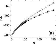
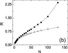
Figure 4: The energy per particle $(a)$ and the maximum radius $(b)$ of the Coulomb dot (solid circles) and the parabolic dot (open triangles) as a function of $N$. The confinement charge of the Coulomb dot is $Z=200$.

More over, if one plots the differences of energy per particle (scaled by $Z$) as a function of the number of particles $N$, as is shown in Fig. 5, we can see small cusps related to the so called “magic numbers” which are known to be an important feature of the configurations of the parabolic dots schweg .

Figure 5: Difference in the energy per particle per $Z$ as a function of $N$ for a Coulomb dot with $Z=100$. Examples of configurations where kinks are found in the energy curve are shown in the insets.

In the opposite case of large electron numbers ($n\lesssim 1$), where the system is nearly neutral, one can expect to find features which are specific for our Coulomb screening case and which are not found with a parabolic dot. In this asymptotic case, the Coulomb dot presents a low density system colloid which is under the influence of a nonhomogeneous electric field. We already know that correlation effects in such a system is of most importance. That is why it is worth to take as a reference the hydrodynamic approach, which is some mean field theory where no correlation effects are included.

IV Hydrodynamic approach

In the hydrodynamic approach the electrons are described by the 2D density $\rho({\bf r})$. They create a potential $\phi({\bf r},z)$ which obey the Poisson equation

$$\nabla^{2}\phi(r,z)=4\pi\rho(r)\delta(z),$$ (6)

in the whole 3D space. Using the dimensionless variables introduced in Sec. II, the electron density is measured in $a^{-2}$ units and the potential in $e/a$ units. Note we took into account the cylinder symmetry of the problem caused by the confining potential $V(r)=-Z/\sqrt{r^{2}+1}$ (see Eq. (2)). The Poisson equation can be replaced by the Laplace equation

$$\nabla^{2}\phi(r,z)=0$$ (7)

everywhere outside the $xy$-plane together with the boundary condition

$$\left.\frac{\partial\phi(r,z)}{\partial z}\right|_{z=0}=2\pi\rho(r)$$ (8)

on this plane.

The mathematical model is based on the statement that the electrons (located in the circular disk of radius $R$) have the same energy in every point of the dot, namely,

$$\left\{V(r)-\phi(r)\right\}\Big{|}_{r<R}=\mu=\mathrm{const}.$$ (9)

Here the symbol $\phi({\bf r})=\phi({\bf r},0)$ stands for the potential created by the 2D electrons in the disk, and the symbol $\mu$ is the chemical potential of this electron system.

The above equations have to be supplemented with one more expression, namely, the conservation of the total number of electrons

$$N=2\pi\int_{0}^{R}rdr\rho(r).$$ (10)

The hydrodynamic approach is a kind of mean field theory where no correlation effects are included. For instance, the phenomena of overcharging colloid cannot take place, and the condition $n=N/Z\leq 1$ is always satisfied, namely, the number of electrons $N$ attracted by the Coulomb center never exceeds its charge number $Z$. The specific case $n=1$ is referred to as complete screening. In this case the analytical solution of the above equations can be obtained using the mirror charge technique, and it leads to the following result

$$\rho_{\mathrm{cs}}(r)=\displaystyle{\frac{1}{2\pi(r^{2}+1)^{3/2}}},$$ (11)

with $n_{\mathrm{cs}}=1$ and $\mu_{\mathrm{cs}}=0$. This simple limiting case result is useful as a reference.

In the general $N<Z$ case we solved the hydrodynamic equations using the oblate spherical coordinates ($0<\tau<1,\,0<\sigma<\infty$) which are defined by

$$x = R\sqrt{(\sigma^{2}+1)(1-\tau^{2})}\cos\theta,$$ (12a)

$$y = R\sqrt{(\sigma^{2}+1)(1-\tau^{2})}\sin\theta,$$ (12b)

$$z = R\sigma\tau$$ (12c)

as it was done in Refs. ye94 ; partoens98 for the case of a parabolic dot with radius $R$. The solution of the Laplace equation (7) can be presented as an expansion

$$\phi(r,z)=\Phi(\tau,\sigma)=\sum_{n=0}^{\infty}C_{n}P_{2n}(\tau)\frac{Q_{2n}(i\sigma)}{Q_{2n}(0)},$$ (13)

in terms of the first $P_{2n}$ and second $Q_{2n}$ kind Legendre polynomials. Thus, the potential created by the electrons on the disk ($\sigma=0,\;\tau<1$) can be presented as

$$\phi(r)=\Phi(\tau)=\sum_{n=0}^{\infty}C_{n}P_{2n}(\tau).$$ (14)

Now taking into account that on the disk we have according to Eq. (12c)

$$\frac{\partial}{\partial z}\Bigg{|}_{z=0}=\frac{1}{R\tau}\frac{\partial}{\partial\sigma}\Bigg{|}_{\sigma=0},$$ (15)

and satisfying the boundary condition (8) one gets the analogous expansion for the electron density

$$\rho(r)=\chi(\tau)=-\frac{1}{2\pi R\tau}\sum_{n=0}^{\infty}C_{n}L_{n}P_{2n}(\tau),$$ (16)

where

$$L_{n}=-\left\{\frac{d}{d\sigma}\ln Q_{2n}(i\sigma)\right\}\Bigg{|}_{\sigma=0}=2\left\{\frac{\Gamma(n+1)}{\Gamma(n+1/2)}\right\}^{2},$$ (17)

and $\Gamma(x)$ is the Gamma function.

Next, we expand the Coulomb center potential on the disk into a series of Legendre polynomials as well

$$V(r)=-\frac{Z}{R\sqrt{1+1/R^{2}-\tau^{2}}}=-\frac{Z}{R}\sum_{n=0}^{\infty}A_{n}P_{2n}(\tau),$$ (18)

and inserting it together with Eq. (14) into Eq. (9) we obtain the final expression

$$C_{n}=-\mu\delta_{n,0}-\frac{Z}{R}A_{n}$$ (19)

for the electron density expansion coefficients $C_{n}$.

In order to define the chemical potential $\mu$ we have to remember that the electron density has to be equal to zero at the free electron system boundary $r=R$. Thus, the electron density should satisfy the following condition

$$\begin{split}2\pi R\lim_{\tau\to 0}\tau\chi(\tau)&=-\sum_{n=0}^{\infty}C_{n}L_{n}P_{2n}(0)\\ &=-\mu L_{0}-\frac{Z}{R}\sum_{n=0}^{\infty}A_{n}L_{n}P_{2n}(0)=0,\end{split}$$ (20)

what finally enables us to define the chemical potential

$$\mu = -\frac{Z}{RL_{0}}\sum_{n=0}^{\infty}A_{n}L_{n}P_{2n}(0)$$ (21)

$$= -\frac{Z\sqrt{\pi}}{R}\sum_{n=0}^{\infty}(-1)^{n}A_{n}\frac{\Gamma(n+1)}{\Gamma(n+1/2)},$$

and write down the following electron density expression

$$\chi(\tau)=\frac{Z}{2\pi R^{2}\tau}\sum_{n=1}^{\infty}A_{n}L_{n}\left\{P_{2n}(\tau)-P_{2n}(0)\right\}.$$ (22)

Inserting the density expression (16) into Eq. (10) one obtains the number of electrons

$$n=\frac{N}{Z}=\frac{2}{\pi}\left(A_{0}+\frac{R}{Z}\mu\right),$$ (23)

taking part in the screening of the Coulomb center.

Equations (18), (21), (22), and (23) actually are the solution of the problem if the coefficients $A_{n}$ are known. These coefficients are calculated in Appendix A.

The density (22) enables us to calculate all properties of the electron system. For instance, the square of mean electron radius can be estimated as

$$<r^{2}>=\frac{1}{N}\int_{0}^{R}dr\,r^{3}\rho(\tau)=R^{2}\left(\frac{2}{3}-\frac{16A_{1}}{15\pi n}\right).$$ (24)

Due to the linear dependence of the confinement potential (18), the chemical potential (21) and the density (22) on the charge number $Z$, it can be removed by a scaling, and the hydrodynamic problem is actually controlled by a single parameter (say, $n$ or $R$) in contrast to the system of discrete electrons for which the two parameters ($Z$ and $N$) were essential. Thus, the general solution can be presented by both chemical potential and density curves, as is shown in Fig. 6 by solid curves.

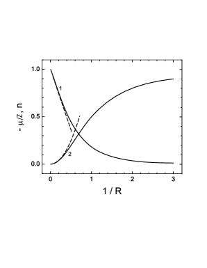
Figure 6: Hydrodynamic solution (solid curves) and its asymptotic (dashed curves) for large $R$: 1 – number of particles (Eq. (23)) , 2 – chemical potential (Eq. (21)).

The corresponding dashed curves indicate the asymptotic of the above quantities

$$\mu_{\mathrm{as}} = -\frac{Z}{R^{2}},$$ (25a)

$$n_{\mathrm{as}} = 1-\frac{4}{\pi R},$$ (25b)

which holds for a nearly neutral ($n\to 1$) electron system. In Fig. 7 the electron density for various dot radii is shown.

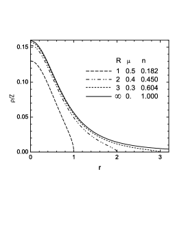
Figure 7: Hydrodynamic solution for the electron density for various dot radii.

We see that in the case of small radius (or equivalently large $Z$, i.e. $n<<1$) the electron density becomes similar to the density in a parabolic dot ($\rho\sim\sqrt{1-r^{2}/R^{2}}$), while in the opposite large radius case it tends to the limiting density (11) for the completely screened case.

V Correlation effects

In order to compare the numerical simulation results with the hydrodynamic approach we scaled them by the charge number $Z$. In Fig. 8(a), the energy per particle scaled by $Z$ is shown as a function of the relative number of electrons $n=N/Z$.

Figure 8: The scaled energy per particle (a) and chemical potential (b) obtained from our numerical simulations for different values of the confinement charge $Z$ are compared with the hydrodynamic result.

The hydrodynamic result (solid curve) was obtained by numerically integrating the scaled chemical potential (21) over the number of electrons $n$, namely,

$$\frac{E(n)}{ZN}=\frac{1}{ZN}\int_{0}^{n}\mu dn.$$ (26)

In Fig. 8(b) the same comparison is shown for the scaled chemical potential. The numerical simulation results were calculated as the difference of the total energies for adjacent configurations, namely, $\mu_{N}=E_{N+1}-E_{N}$. We see that when the charge number $Z$ increases the curves tend towards the hydrodynamic result. This is more clearly seen for the chemical potential (Fig. 8(b)) than for the total energy curves (Fig. 8(a)).

The deviation of the energy and the chemical potential of the ’exact’ numerical simulation results from their hydrodynamic counterparts has to be interpreted as a correlation energy, because such correlations are not included in the hydrodynamic approach. As an example, we show in Fig. 9, for $Z=100$, this difference in energy per particle and similar results for the chemical potential. The curves for other values of the confinement charge demonstrate a similar behavior.

Figure 9: The difference in energy (a) and chemical potential (b) between the hydrodynamic result and the simulation result for $Z=100$.

The most remarkable feature of these curves is the linear behavior in the nearly full screening region ($n\to 1$). The curves in the above region can be fitted by the rather simple analytical expressions:

$$\Delta E/NZ=A_{E}-B_{E}n,$$ (27a)

$$\Delta\mu/Z=A_{\mu}-B_{\mu}n.$$ (27b)

For the results of Fig. 9 we found

$$\Delta E/NZ=0.068-0.034n,$$ (28a)

$$\Delta\mu/Z=0.065-0.067n.$$ (28b)

Although the coefficients of these expressions are $Z$-dependent, we found that the ratio of them are Z-independent ($A_{E}/B_{E}\approx 2$ and $A_{\mu}/B_{\mu}\approx 1$).

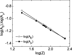
Figure 10: Logarithmic plot of the parameter $A$ of the linear fit of the deviation curves for the energy per particle and the chemical potential in the nearly complete screening limit.

The linear behavior of these curves in the double logarithmic plot, as it is seen in Fig. 10, enables us to fit them by $A=\alpha Z^{-\beta}$. The straight lines in Fig. 10 correspond to $\alpha=0.69$ and $\beta=0.5$ for $A_{E}$, and $\alpha=0.55$ and $\beta=0.46$ for $A_{\mu}$. Therefore, we suggest the following asymptotic behaviour for $N\rightarrow Z$

$$\Delta E/N\sim\sqrt{Z}\left(1-\frac{N}{2Z}\right),$$ (29a)

$$\Delta\mu\sim\sqrt{Z}\left(1-\frac{N}{Z}\right).$$ (29b)

These results express the contribution of correlation to the energy and the chemical potential of our Coulomb bound classical dot.

Qualitatively, such dependence can be explained by means of the crystallization energy which can be estimated as

$$E_{\mathrm{cr}}=\int_{0}^{R}d^{2}r\rho(r)E_{I}(r)$$ (30)

where $E_{I}(r)$ is the local density crystallization energy which we approximated by the result from a homogeneous Wigner crystal bonsal77

$$E_{I}=a_{0}\sqrt{\rho}.$$ (31)

The coefficient equals $a_{0}\approx 3.921$ for the triangular lattice. Now inserting the above expression into Eq. (30), replacing the electron density by its asymptotic expression (11), and taking Eq. (25b) into account we obtained the following estimate:

$$E_{\mathrm{cr}} \approx 2\pi a_{0}\int_{0}^{R}rdr\rho_{\mathrm{cs}}^{3/2}=\frac{a_{0}Z^{3/2}}{\sqrt{2\pi}}\int_{0}^{R}\frac{rdr}{(r^{2}+1)^{9/4}}$$ (32)

$$= \frac{2a_{0}Z^{3/2}}{5\sqrt{2\pi}}\left\{1-\left[\frac{\pi}{4}(1-n)\right]^{5/2}\right\}.$$

Taking only the first term into account and dividing the above crystallization energy by $N=Z\{1-(1-n)\}$ we obtained the following approximate crystallization energy per particle

$$\frac{E_{cr}}{N}\approx\frac{2a_{0}\sqrt{Z}}{5\sqrt{2\pi}}(2-n),$$ (33)

which demonstrates the same parameter dependencies as obtained earlier, Eq. (29a), from a fitting of our simulation results.

Differentiating the above crystallization energy expression by $n$ we also obtained an estimation for the correlation contribution to the chemical potential:

$$\mu_{cr}=\frac{d}{dN}E_{cr}=\frac{2a_{0}\sqrt{Z}}{5\sqrt{2\pi}}\frac{d}{dn}n(2-n)\sim\sqrt{Z}(1-n)$$ (34)

which coincides with our earlier result, Eq. (29b).

Unfortunately, no similar simple expressions can be obtained for the dot radius as depicted in Fig. 11. We see that the radii from the hydrodynamic approach and the discrete system differs substantially, and the deviation grows in the limiting $n\to 1$ case. The discrete system is more compact as compared with the continuous one, which is an indication that the discrete system may lead to overcharging colloid which cannot be described by a hydrodynamic theory.

Figure 11: Comparison of maximal ($R$) and mean radii ($r$) of the electron system obtained from the numerical simulation (for different $Z$-values) and in the hydrodynamic approach as function of $n=N/z$. The Z-dependence of the maximum and the mean radius is enlarged in the inset.

VI Conclusions

We studied numerically the ground state properties of a 2D model system consisting of classical charged particles which are Coulomb bound. This system is similar to an atomic system. The $N$ electrons moving in a plane are confined through a positive remote impurity potential of charge $Z$. The configurations for $n\ll N/Z$ are similar to those of a parabolic confined dot, but for $n\sim 1$ they are very different, with an inner core consisting of approximately a triangular lattice and an outer region with particles situated on a ring.

A hydrodynamic analysis of the problem clearly emphasizes the importance of correlation effects between the negatively charges particles. Furthermore, analytical expressions for the correlation energy contributions to the total energy and the chemical potential were obtained in the limit of nearly overscreening, e. g. $n\sim 1$. Those analytical results compare favorably well with our numerical “exact” simulation results.

Appendix A Coulomb potential expansion coefficients

According to Eq. (18) the Coulomb potential expansion coefficients $A_{n}$ depend on the single variable $b=1/R$, and they can be calculated straightforwardly. Indeed, multiplying Eq. (18) by $P_{2m}(\tau)$, integrating it over $\tau$ and using the normalization integral for symmetric Legendre polynomials one obtains the following integral expression:

$$A_{n}(b)=(4n+1)\int_{0}^{1}\frac{P_{2n}(\tau)d\tau}{\sqrt{1+b^{2}-\tau^{2}}}.$$ (35)

The most accurate way to calculate the above integral is to expand the denominator into a $\tau^{2n}$ power series and use the analytical expression for

$$\int_{0}^{1}x^{2k}P_{2n}(x)dx=\frac{(-1)^{n}\Gamma(n-k)\Gamma(k+1/2)}{2\Gamma(-k)\Gamma(n+k+3/2)},$$ (36)

what enables us to convert the integral (35) into the following sum

$$A_{n}(b) = \frac{(4n+1)}{2\sqrt{\pi}\,(1+b^{2})^{n+1/2}}$$ (37)

$$\times\sum_{m=0}^{\infty}\frac{\Gamma^{2}(m+n+1/2)(1+b^{2})^{-m}}{\Gamma(m+1)\Gamma(m+2n+3/2)}.$$

The convergence of this sum is rather slow. Fortunately, it can be improved by adding the asymptotic, namely, replacing Eq. (37) by the following expression

$$A_{n}(b) = \frac{(4n+1)}{2\sqrt{\pi}\,(1+b^{2})^{n+1/2}}$$ (38)

$$\times \sum_{m=0}^{s}\frac{\Gamma^{2}(m+n+1/2)(1+b^{2})^{-m}}{\Gamma(m+1)\Gamma(m+2n+3/2)}$$

$$+ \frac{4n+1}{(1+b^{2})^{s+n+1/2}}$$

$$\times \left\{\frac{1}{\sqrt{\pi s}}-b\,e^{b^{2}s}\left[1-\Phi(b\sqrt{s})\right]\right\}.\phantom{m}$$

where $s$ is an integer which should be optimized for rapid convergence and $\Phi(z)$ is the error function. The above expression is very convenient and enables us to obtain good accuracy in a fast way if one uses the recurrence expressions for the calculations of the gamma functions (as for the Legendre polynomials in Eq. (22) as well).