Towards local rheology of emulsions under Couette flow using Dynamic Light Scattering

Abstract

We present local velocity measurements in emulsions under shear using heterodyne Dynamic Light Scattering. Two emulsions are studied: a dilute system of volume fraction $\phi=20$ % and a concentrated system with $\phi=75$ %. Velocity profiles in both systems clearly show the presence of wall slip. We investigate the evolution of slip velocities as a function of shear stress and discuss the validity of the corrections for wall slip classically used in rheology. Focussing on the bulk flow, we show that the dilute system is Newtonian and that the concentrated emulsion is shear-thinning. In the latter case, the curvature of the velocity profiles is compatible with a shear-thinning exponent of 0.4 consistent with global rheological data. However, even if individual profiles can be accounted for by a power-law fluid (with or without a yield stress), we could not find a fixed set of parameters that would fit the whole range of applied shear rates. Our data thus raise the question of the definition of a global flow curve for such a concentrated system. These results show that local measurements are a crucial complement to standard rheological tools. They are discussed in light of recent works on soft glassy materials.

1 Introduction

Emulsions are mixtures of two immiscible fluids. They are usually formed by mechanical mixing and consist of droplets of one fluid dispersed in the other. They are metastable so that the mean size of the droplets tends to increase with time. Emulsions belong to a wide class of non-equilibrium systems such as foams that rearrange and coarsen with time Larson:1999 . The use of surfactants or polymers increases the characteristic time for coarsening of emulsions from a few seconds to a few years and make them very attractive for applications such as road building, pharmacology or food processing. They constitute very interesting tools to entrap hazardous solvents, to carry additives or to change the rheological properties of a sample. Indeed, their rheological characteristics may be tuned by increasing the liquid fraction of the dispersed phase.

When the liquid fraction is low, the droplets of the emulsion are Brownian and the emulsion is a Newtonian fluid whose viscosity is close to that of the continuous phase. When the liquid fraction is increased, less space is available to each particle. The droplets are pressed against each other, their shape are distorted, and energy is stored at their interfaces. For small deformations, the droplets resist shear elastically. Such elasticity results from the energy stored by additional deformation of their shape induced by the applied strain. For large deformations, they flow irreversibly.

Mason et al. Mason:1996a have shown that this change of regime occurs above a critical stress and that, for concentrated emulsions in the neighbourhood of this critical stress, the flow may become inhomogeneous. In Ref. Mason:1996a , the homogeneity of the flow was determined by painting a stripe on the exposed surface of the emulsion before shearing and by following its evolution under shear. Moreover, the analysis of the rheological data may be complicated by the existence of slippage of the emulsion at the walls Barnes:1994 .

Due to all these difficulties, local measurements of the velocity are needed to characterize the flow of the emulsion once it has yielded. Recently, Coussot et al. Coussot:2002 measured velocity profiles of various colloidal systems such as gels, laponite solutions or industrial emulsions by imaging the flow field with Magnetic Resonance Imaging (MRI). They described the yield stress phenomenon as an abrupt transition between two distinct states: a liquid-like state that flows, and a solid-like state that remains jammed and does not flow. The rheological behaviour of the liquid state was modelled by that of a power-law fluid.

In this article, we present measurements of velocity profiles in sheared emulsions using Dynamic Light Scattering (DLS) in the heterodyne geometry. Our setup allows us to perform both global rheological measurements and local velocity measurements simultaneously. We study two different oil-in-water emulsions: a dilute emulsion of volume fraction $\phi=20~{}\%$ and a concentrated one at $\phi=75~{}\%$. In both cases, we get a quantitative measure of wall slip and show the importance of this phenomenon. We point out that corrections for slippage like those proposed by Mooney and classically used in rheological experiments are indeed well suited for concentrated emulsions but may fail for dilute systems. In the case of the concentrated emulsion, we show the existence of two regimes separated by an abrupt transition between a jammed state and a flowing phase like Coussot et al Coussot:2002 . However, in our case, no clear analytical flow curve could be obtained for the whole range of shear rates investigated in the present study.

In the next Section of this article, we describe the method used for preparing the samples. The third Section briefly recalls our experimental technique and setup for measuring the local velocity of a complex fluid in a Couette flow Salmon:2002pp . We then present the velocity profiles obtained in the two emulsions under shear. Finally, we discuss both the slippage and the yield stress phenomena in our emulsions.

2 Preparation of the emulsions under study

We prepare a crude emulsion of fixed composition by gently shear-mixing 400 g of silicone oil (Polydymethyl Siloxane of viscosity 135 Pa.s from Rhodia), 30.3 g of glycerol, 30.3 g of water and 9.9 g of surfactant (Tetradecyl Trimethyl Ammonium Bromide from Aldrich). The aqueous phase is thus composed of a 14 % wt. solution of TTAB in a 1:1 mixture of water and glycerol. The resulting polydisperse viscoelastic premixed emulsion of large droplets is sheared within a narrow gap in a laminar regime Mason:1996b .

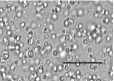
Figure 1: Photograph of the emulsion under study. The concentrated emulsion was diluted in order to visualize individual droplets using a microscope (magnification $\times$50). The black bar represents 20 $\mu$m.

The mother emulsion obtained after shearing is composed of monodisperse silicone oil droplets of diameter $2~{}\mu$m in the water–glycerol–surfactant mixture (see Fig. 1). Then, by dilution, we set the surfactant concentration within the water–glycerol phase to $1~{}\%$ in mass and concentrate the droplets by centrifugation to a volume fraction of $\phi=75~{}\%$, such that droplets are compressed one against another leading to flat films at each contact. We chose this surfactant concentration in order to ensure a good stability to the emulsion. This concentration is high enough to prevent coalescence and small enough to avoid flocculation by depletion. We prepare another emulsion with a volume fraction $\phi=20~{}\%$ by diluting the concentrated one in the water–glycerol–surfactant solution. The surfactant concentration is kept equal to $1~{}\%$.

The use of a water–glycerol mixture allows us to match the optical index $n$ of the continuous phase of the emulsion to that of the silicone oil ($n=1.40$). The obtained emulsions are thus nearly transparent and do not present any significant multiple light scattering. The emulsion is then carefully loaded into the transparent Couette cell of a rheometer (see below). For the whole range of applied shear rates, we check by optical microscopy that the structure of the emulsion and the size of the droplets are not affected by shear and that no noticeable coalescence takes place.

3 Experimental setup for heterodyne DLS in Couette flows

In order to measure the local velocity of emulsions in Couette flows, we used the experimental technique based on heterodyne DLS described at length in a related work Salmon:2002pp . In this Section, we briefly recall the basics of heterodyne DLS and the setup developed in our laboratory to perform local velocity measurements. The reader is referred to Ref. Salmon:2002pp for more details on the optics of this setup and for a complete discussion on the resolution of heterodyne DLS.

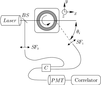
Figure 2: Simplified heterodyne DLS setup. $BS$ denotes a beam splitter, $SF$ spatial filters, and $C$ the device coupling optical fibers and used to perform the interference between the scattered light and the reference beam.

Local velocity measurements using heterodyne DLS relie on the detection of the Doppler frequency shift associated with the motion of the scatterers inside a small scattering volume $\mathcal{V}$ Berne:1995 ; Ackerson:1981 ; Gollub:1974 . In classical heterodyne setups, light scattered by the sample under study is collected along a direction $\theta$. The scattering volume is defined as the intersection between the incident beam and the scattered beam. The scattered electric field is then made to interfere with a reference beam. Finally, light resulting from the interference is sent to a photomultiplier tube (PMT) and the auto-correlation function of the intensity is computed using an electronic correlator. The originality of our setup lies in the use of single mode fibers to collect scattered light, to perform the interference, and to carry light to the PMT. This allows for great flexibility when choosing the scattering angle. Figure 2 sketches the main features of such a setup.

When the scattering volume $\mathcal{V}$ is submitted to a shear flow, it can be shown that the correlation function $C(\tau)$ is an oscillating function of the time lag $\tau$ modulated by a slowly decreasing envelope. The frequency of the oscillations in $C(\tau)$ is exactly the Doppler shift $\mathbf{q}\cdot\mathbf{v}$, where $\mathbf{q}$ is the scattering wavevector and $\mathbf{v}$ is the local velocity averaged over the size of the scattering volume which is about 100 $\mu$m in our experiments. Figure 3 shows a typical correlation function measured on a sheared emulsion. The frequency shift $\mathbf{q}\cdot\mathbf{v}$ is recovered by interpolating a portion of $C(\tau)$ and looking for the zero crossings. Error bars on such measurements are obtained by varying the number of zeros taken into account in the analysis. Typical uncertainties are about 5 %.

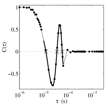
Figure 3: Experimental heterodyne correlation function ($\bullet$) recorded on the concentrated emulsion at $\dot{\gamma}=10$ s^-1. The thick line shows the portion of the heterodyne function from which the frequency shift $\mathbf{q}\cdot\mathbf{v}$ is calculated.

Couette flows are generated between two cylinders in a transparent Mooney-Couette cell. The radius of the rotating inner cylinder (“rotor”) is $R_{\scriptscriptstyle 1}=22$ mm and the radius of the fixed outer cylinder (“stator”) is $R_{\scriptscriptstyle 2}=25$ mm leaving a gap $e=R_{\scriptscriptstyle 2}-R_{\scriptscriptstyle 1}=3$ mm between the two cylinders. The length of the cylinders is $H=30$ mm. Both cylinders are in Plexiglas and have smooth surfaces so that wall slip is likely to occur in our experiments. The rotation of the moving cylinder is imposed by a classical rheometer (TA Instruments AR1000) operated in the “imposed shear rate” mode. This rheometer measures both the torque $\Gamma$ on the inner cylinder and its angular velocity $\Omega$ in real-time. From $\Omega$ and $\Gamma$, it also computes a global shear rate $<\dot{\gamma}>$ and shear stress $<\sigma>$ using the formulas:

$$<\dot{\gamma}> = \frac{R_{\scriptscriptstyle 1}^{2}+R_{\scriptscriptstyle 2}^{2}}{R_{\scriptscriptstyle 2}^{2}-R_{\scriptscriptstyle 1}^{2}}\,\Omega\,,$$ (1)

$$<\sigma> = \frac{R_{\scriptscriptstyle 1}^{2}+R_{\scriptscriptstyle 2}^{2}}{4\pi HR_{\scriptscriptstyle 1}^{2}R_{\scriptscriptstyle 2}^{2}}\,\Gamma\,.$$ (2)

In the following, the results will be presented in terms of $<\dot{\gamma}>$ and $<\sigma>$ which will simply be noted $\dot{\gamma}$ and $\sigma$, as is usually done in rheology. Using Eq. (1), the velocity of the moving wall $v_{\scriptscriptstyle 0}=R_{\scriptscriptstyle 1}\Omega$ is given by:

$$v_{\scriptscriptstyle 0}=\frac{R_{\scriptscriptstyle 1}(R_{\scriptscriptstyle 1}+R_{\scriptscriptstyle 2})}{R_{\scriptscriptstyle 1}^{2}+R_{\scriptscriptstyle 2}^{2}}\,\dot{\gamma}e\,.$$ (3)

Thus, in the Couette geometry used in the present work, one has to keep in mind that $v_{\scriptscriptstyle 0}\approx 0.93\,\dot{\gamma}e$ so that $v_{\scriptscriptstyle 0}$ differs from $\dot{\gamma}e$ by about 7 %.

The temperature of the sample is controlled within $\pm\,0.1^{\circ}$C using a water circulation around the cell. The rheometer sits on a mechanical table whose displacements are controlled by a computer. Three mechanical actuators allow us to move the rheometer in the $x$, $y$, and $z$ directions with a precision of $1~{}\mu$m. Once $y$ and $z$ are set so that the incident beam is normal to the cell surface, velocity profiles are measured by moving the mechanical table in the $x$ direction by steps of 50 or 100 $\mu$m.

As discussed in Ref. Salmon:2002pp , going from $\mathbf{q}\cdot\mathbf{v}$ as a function of the table position $x_{t}$ to the velocity profile $v(x)$ (where $x$ is the radial position of the scattering volume $\mathcal{V}$ within the sample) requires a careful calibration procedure. Indeed, refraction effects due to the curved geometry of the Couette cell lead to significant differences between the angle $\theta_{i}$ imposed by the operator and the actual scattering angle $\theta$ in the sample, and between the table displacement $\delta x$ and the actual displacement $\delta x^{\prime}$ of $\mathcal{V}$. By using a Newtonian suspension of latex spheres in a water–glycerol mixture (optical index $n=1.40$) at various known shear rates, we showed that for $\theta_{i}=35^{\circ}$, $\theta=f_{\theta}\,\theta_{i}$ and $\delta x^{\prime}=f_{x}\,\delta x$ with $f_{\theta}\approx 0.79$ and $f_{x}\approx 1.13$.

When loading the cell with the emulsions, great care is taken to ensure that the position of the Couette cell does not change between the calibration with the latex suspension and the actual experiments on emulsions. Since the optical index of the fluid is $n=1.40$ in both cases, the above values of $f_{x}$ and $f_{\theta}$ found with the latex suspension are used to convert raw data $(\mathbf{q}\cdot\mathbf{v})(x_{t})$ into velocity profiles $v(x)$ in the case of our emulsions. Finally, we chose to accumulate the correlation functions over 1 min so that a full velocity profile with a resolution of 100 $\mu$m takes about 30 min to complete. Note that our setup allows us to record rheological data and the local velocity at the same time on the same sample. In all the cases described below, we checked that steady state was reached from the curves $\dot{\gamma}(t)$ and $\sigma(t)$.

4 Velocity profiles in sheared emulsions

4.1 Dilute emulsion ($\phi=20~{}\%$)

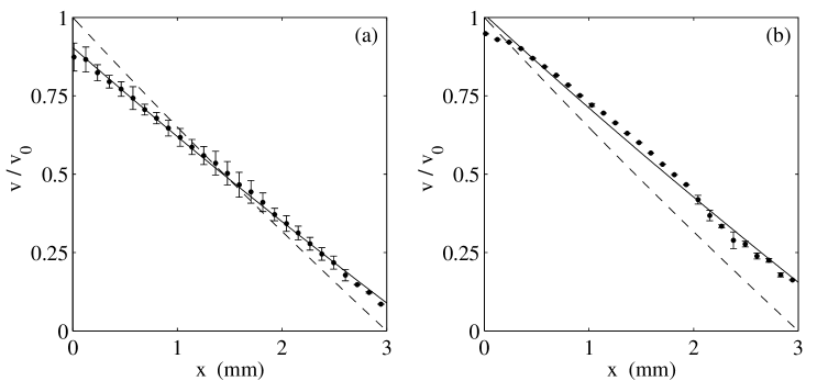
Figure 4: Velocity profiles in the 20 % emulsion for (a) $\dot{\gamma}=0.1$ s^-1 and (b) $\dot{\gamma}=0.2$ s^-1. The solid curves are the best fits to the data using Eq. (15) with $n=1$. The dashed lines represent the velocity profiles expected for a Newtonian fluid.

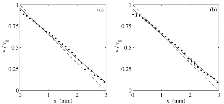
Figure 5: Velocity profiles in the 20 % emulsion for (a) $\dot{\gamma}=0.4$ s^-1 and (b) $\dot{\gamma}=1$ s^-1. The solid curves are the best fits to the data using Eq. (15) with $n=1$. The dashed lines represent the velocity profiles expected for a Newtonian fluid.

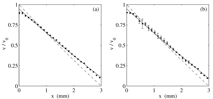
Figure 6: Velocity profiles in the 20 % emulsion for (a) $\dot{\gamma}=2$ s^-1 and (b) $\dot{\gamma}=5$ s^-1. The solid curves are the best fits to the data using Eq. (15) with $n=1$. The dashed lines represent the velocity profiles expected for a Newtonian fluid.

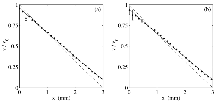
Figure 7: Velocity profiles in the 20 % emulsion for (a) $\dot{\gamma}=10$ s^-1 and (b) $\dot{\gamma}=15$ s^-1. The solid curves are the best fits to the data using Eq. (15) with $n=1$. The dashed lines represent the velocity profiles expected for a Newtonian fluid.

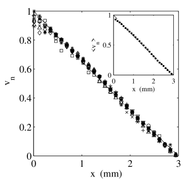
Figure 8: Normalized velocity profiles measured in the 20 % emulsion for $\dot{\gamma}=0.1$ s${}^{-1}~{}(\triangledown)$, 0.2 s${}^{-1}~{}(\triangle)$, 0.4 s${}^{-1}~{}(+)$, 1 s${}^{-1}~{}(\times)$, 2 s${}^{-1}~{}(\circ)$, 5 s${}^{-1}~{}(\Box)$, 10 s${}^{-1}~{}(\bullet)$, 15 s${}^{-1}~{}(\diamond)$, and 20 s${}^{-1}~{}(\ast)$. Each profile is normalized according to $v_{n}=(v-v_{\scriptscriptstyle 2})/(v_{\scriptscriptstyle 1}-v_{\scriptscriptstyle 2})$. The dashed line is the result expected for a Newtonian fluid. Inset: the average of the previous normalized profiles $<v_{n}>$ ($\bullet$) compared to the Newtonian prediction (dashed line).

Figures 4–7 present the velocity profiles measured in the dilute emulsion of liquid fraction $\phi=20~{}\%$ for various imposed shear rates ranging from $0.1$ s^-1 to $15$ s^-1. The velocity profiles expected for a Newtonian fluid are shown as dashed lines. The velocities $v(x)$ have been rescaled by the inner wall velocity $v_{\scriptscriptstyle 0}$. In these figures, the upper left corner (at $x=0$) thus always corresponds to the velocity of the inner wall moving at $v_{\scriptscriptstyle 0}$, and the lower right corner (at $x=e=3$ mm) to the fixed outer wall ($v=0$). First, one can notice that the experimental velocity is always different from zero at the stator and different from the rotor velocity at the rotor. This means that significant slippage occurs and remains of the order of $10~{}\%$ of $v_{\scriptscriptstyle 0}$. We define the slip velocity at the rotor $v_{s_{1}}=v_{\scriptscriptstyle 0}-v_{\scriptscriptstyle 1}$ as the difference between the rotor velocity $v_{\scriptscriptstyle 0}$ and the emulsion velocity $v_{\scriptscriptstyle 1}$ at the rotor and the slip velocity $v_{s_{2}}=v_{\scriptscriptstyle 2}$ at the stator as the emulsion velocity $v_{\scriptscriptstyle 2}$ at the stator.

Moreover, all the velocity profiles measured in the dilute emulsion are linear. To better illustrate this point, Fig. 8 presents the normalized velocity $v_{n}$ for various applied shear rates. We define $v_{n}$ experimentally by:

$$v_{n}(x)\,\widehat{=}\,\frac{v(x)-v_{2}}{v_{1}-v_{2}}\,.$$ (4)

All normalized data coincide and the average master curve $<v_{n}>$ is almost perfectly linear across the cell gap (see inset of Fig. 8). These qualitative results show that, although subject to small but measurable wall slip, the dilute emulsion flows like a Newtonian fluid in the range of shear rates under study.

4.2 Concentrated emulsion ($\phi=75~{}\%$)

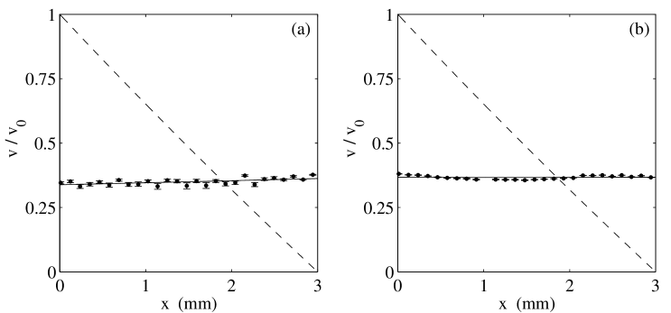
Figure 9: Velocity profiles in the 75 % emulsion for (a) $\dot{\gamma}=0.1$ s^-1 and (b) $\dot{\gamma}=0.2$ s^-1. The solid lines are linear fits to the data. The dashed curves represent the velocity profiles expected for a Newtonian fluid.

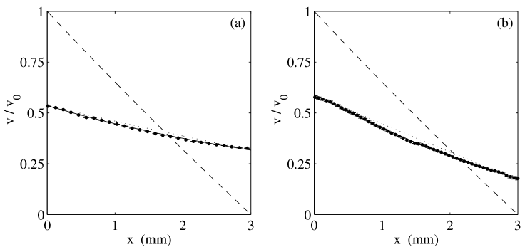
Figure 10: Velocity profiles in the 75 % emulsion for (a) $\dot{\gamma}=0.4$ s^-1 and (b) $\dot{\gamma}=1$ s^-1. The solid curves are the best fits to the data using Eq. (15) with $n=0.4$. The dashed lines represent the velocity profiles expected for a Newtonian fluid. The dotted lines correspond to the case of a Newtonian fluid that would slip at the cell walls with the same velocities as the emulsion.

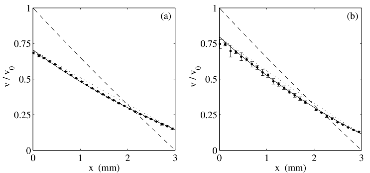
Figure 11: Velocity profiles in the 75 % emulsion for (a) $\dot{\gamma}=2$ s^-1 and (b) $\dot{\gamma}=5$ s^-1. The solid curves are the best fits to the data using Eq. (15) with $n=0.4$. The dashed lines represent the velocity profiles expected for a Newtonian fluid. The dotted lines correspond to the case of a Newtonian fluid that would slip at the cell walls with the same velocities as the emulsion.

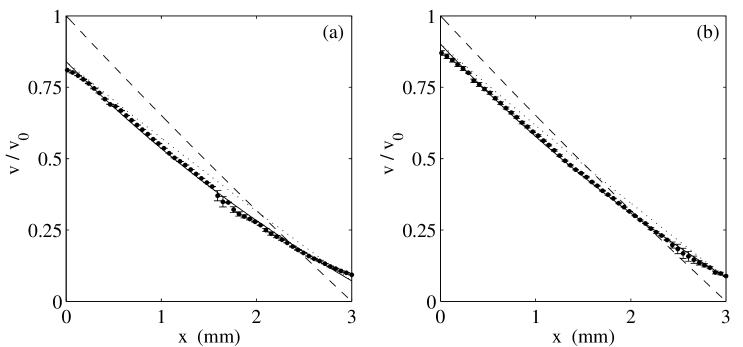
Figure 12: Velocity profiles in the 75 % emulsion for (a) $\dot{\gamma}=10$ s^-1 and (b) $\dot{\gamma}=15$ s^-1. The solid curves are the best fits to the data using Eq. (15) with $n=0.4$. The dashed lines represent the velocity profiles expected for a Newtonian fluid. The dotted lines correspond to the case of a Newtonian fluid that would slip at the cell walls with the same velocities as the emulsion.

Figures 9–12 present the velocity profiles in the concentrated emulsion of liquid fraction $\phi=75~{}\%$ for the previous range of imposed shear rates. Two kinds of behaviours are encountered. In the case of low applied shear rates ($0.1$ and $0.2$ s^-1, see Fig. 9), the emulsion moves around in the gap as a solid body with angular velocity $\omega=0.042$ rad.s^-1 for $\dot{\gamma}=0.1$ s^-1 and $\omega=0.084$ rad.s^-1 for $\dot{\gamma}=0.2$ s^-1. In this regime, all the material actually experiencing shear is located inside thin boundary layers at the two walls. These boundary layers cannot be resolved with our spatial resolution of about 100 $\mu$m. When the applied shear rate is increased, the velocity profiles change. Wall slip remains very important but the emulsion no longer behaves as a solid body. Shear occurs not only in the boundary layers but also in the bulk material.

The velocity profiles are no longer linear but rather curved (see Fig. 11 for instance). Moreover, as shown in Fig. 13, the data for the normalized velocity $v_{n}(x)$ still collapse rather well on a single curve provided the applied shear rate is greater than $0.2$ s^-1. The curvature of the mean normalized profile $<v_{n}>$ is clearly visible in the inset of Fig. 13. This result means that the non-Newtonian features of our concentrated emulsion are strong enough to show up at a local level even in a gap as small as 3 mm.

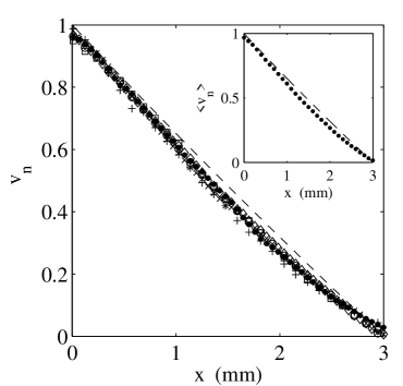
Figure 13: Normalized velocity profiles measured in the 75 % emulsion for $\dot{\gamma}=0.4$ s${}^{-1}~{}(+)$, 1 s${}^{-1}~{}(\times)$, 2 s${}^{-1}~{}(\circ)$, 5 s${}^{-1}~{}(\Box)$, 10 s${}^{-1}~{}(\bullet)$, and 15 s${}^{-1}~{}(\diamond)$. Each profile is normalized according to $v_{n}=(v-v_{\scriptscriptstyle 2})/(v_{\scriptscriptstyle 1}-v_{\scriptscriptstyle 2})$. The dashed line is the result expected for a Newtonian fluid. Inset: the average of the previous normalized profiles $<v_{n}>$ ($\bullet$) compared to the Newtonian prediction (dashed line).

In the next Section, we first discuss the evolution of the slip velocities and then analyze the features of individual velocity profiles in more depth.

5 Local rheology of emulsions in a Couette flow

5.1 Wall-slip and wetting films

For both the dilute and the concentrated emulsions, slippage clearly occurs. The simplest picture one could imagine to describe this situation is the existence of two very thin films of continuous phase near the walls and a bulk material with the original concentration in between Princen:1985 ; Barnes:1995 . From our measurements, it is possible to access the thickness $h$ of the thin film where shear occurs. Indeed, assuming a slip velocity $v_{s}$ within a thin liquid film of viscosity $\eta_{f}$, we may write: $\sigma=\eta_{f}\dot{\gamma}_{s}=\eta_{f}v_{s}/h$, where $\dot{\gamma}_{s}=v_{s}/h$ is the shear rate inside the film. Using the subscript $i=1$ or 2 to denote the film at the rotor or at the stator respectively,

$$h_{i}=\frac{\eta_{f}v_{s_{i}}}{\sigma_{i}}\,\,\,\hbox{\rm for}\,\,\,i=1\,\,\,\hbox{\rm or}\,\,\,2\,,$$ (5)

where $\sigma_{i}$ is the shear stress near wall number $i$. Note that, in the Couette geometry, the values of $\sigma_{i}$ at the walls are linked to the global stress $\sigma$ indicated by the rheometer according to:

$$\sigma_{i}=\frac{2R_{j}^{2}}{R_{\scriptscriptstyle 1}^{2}+R_{\scriptscriptstyle 2}^{2}}\,\sigma\,,$$ (6)

where $j=2$ (resp. $j=1$) when $i=1$ (resp. $i=2$). For each value of $\dot{\gamma}$, the steady-state value of $\sigma$ imposed by the rheometer is recorded and $\sigma_{\scriptscriptstyle 1}$ and $\sigma_{\scriptscriptstyle 2}$ are computed from Eq. (6). In our case, this leads to significant deviations from $\sigma$: $\sigma_{\scriptscriptstyle 1}=1.13\,\sigma$ and $\sigma_{\scriptscriptstyle 2}=0.87\,\sigma$.

5.1.1 Dilute emulsion ($\phi=20~{}\%$)

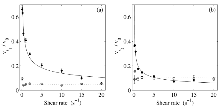
Figure 14: Wall slip velocities for the 75 % emulsion ($\bullet$) and the 20 % emulsion ($\circ$) vs. shear rate. (a) Normalized slip velocity $v_{s_{1}}/v_{\scriptscriptstyle 0}$ at the moving inner wall ($x=0$). The solid line is the power law $0.35\,\dot{\gamma}^{-0.4}$. The dotted line shows the mean value $v_{s_{1}}=0.048\,v_{\scriptscriptstyle 0}$ for the 20 % emulsion. (b) Normalized slip velocity $v_{s_{2}}/v_{\scriptscriptstyle 0}$ at the fixed outer wall ($x=3$ mm). The solid line is the power law $0.20\,\dot{\gamma}^{-0.4}$. The dotted line shows the mean value $v_{s_{2}}=0.10\,v_{\scriptscriptstyle 0}$ for the 20 % emulsion.

In the dilute system, the normalized slip velocities at the rotor $v_{s_{1}}/v_{\scriptscriptstyle 0}$ and at the stator $v_{s_{2}}/v_{\scriptscriptstyle 0}$ are independent of the applied shear rate as can be checked on Fig. 14. This means that $v_{s_{i}}\sim\dot{\gamma}$ and since the dilute emulsion has a Newtonian behaviour, one expects $v_{s_{i}}\sim\sigma_{i}$. This scaling law is indeed observed on Fig. 15(a).

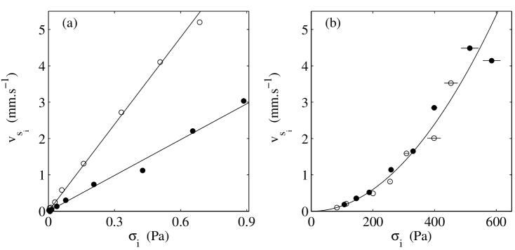
Figure 15: Slip velocities vs. shear stress: $v_{s_{1}}$ vs. $\sigma_{\scriptscriptstyle 1}$ at the rotor ($\bullet$) and $v_{s_{2}}$ vs. $\sigma_{\scriptscriptstyle 2}$ at the stator ($\circ$). (a) For the 20 % emulsion. The straight lines correspond to $v_{\scriptscriptstyle 1}=33\sigma_{\scriptscriptstyle 1}$ and to $v_{\scriptscriptstyle 2}=8.0\sigma_{\scriptscriptstyle 2}$. (b) For the 75 % emulsion. The solid line is $v_{i}=1.5.10^{-5}\,\sigma_{i}^{2}$.

Assuming that the films contain only water and glycerol, one has $\eta_{f}=0.01$ Pa.s. The thicknesses of the films $h_{\scriptscriptstyle 1}$ and $h_{\scriptscriptstyle 2}$ calculated from Eq. (5) are shown as functions of $\sigma_{\scriptscriptstyle 1}$ and $\sigma_{\scriptscriptstyle 2}$ in Fig. 16(a). One gets $h_{\scriptscriptstyle 1}\approx 30~{}\mu$m at the rotor and $h_{\scriptscriptstyle 2}\approx 80~{}\mu$m at the stator independent of the shear stress, which is again consistent with a Newtonian behaviour. Remarkably, these values are much higher than the diameter of the droplets ($2~{}\mu$m), meaning that depletion in the dilute emulsion extends very far from the walls. Various explanations may be proposed for such a large depletion effect.

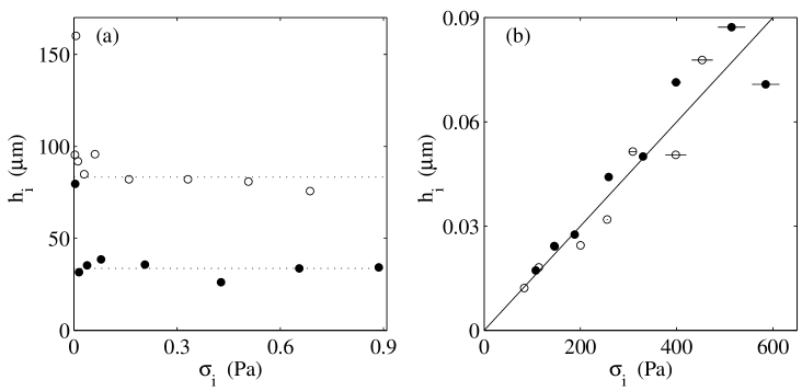
Figure 16: Thickness of the sliding layers vs. shear stress: $h_{\scriptscriptstyle 1}$ vs. $\sigma_{\scriptscriptstyle 1}$ at the rotor ($\bullet$) and $h_{\scriptscriptstyle 2}$ vs. $\sigma_{\scriptscriptstyle 2}$ at the stator ($\circ$). (a) For the 20 % emulsion. The dashed lines are $h_{\scriptscriptstyle 1}=34~{}\mu$m and $h_{\scriptscriptstyle 2}=83~{}\mu$m. (b) For the 75 % emulsion. The solid line corresponds to $h_{i}=1.5.10^{-4}\,\sigma_{i}$.

First, depletion on such long distances might be induced by cumulative effects of inertial effect and of cross-stream migration. Indeed, Goldsmith and Mason reported rapid migration from walls of neutrally buoyant and deformable droplets in pipe and Couette flows Goldsmith:1962 . The authors suggest that such a migration could be initiated by the presence of the wall and of non-uniform velocity gradients. A net force acting to push the drop to a lower gradient is created.

Second, it is important to note that the viscosity of the emulsion varies dramatically with oil concentration. For example, the viscosity of the 20 % emulsion indicated by the rheometer is 0.037 Pa.s. When diluted to a volume fraction $\phi=10~{}\%$, the viscosity decreases to 0.017 Pa.s. Finally, at $\phi=5~{}\%$, the viscosity is equal to 0.011 Pa.s, very close to that of the continuous phase. This means that the lubricating layers could also be viewed as emulsion films with a concentration gradient, for example from $\phi=20~{}\%$ in the bulk to $\phi<5~{}\%$ near the walls, rather than a film of pure continuous phase. This would reduce greatly the magnitude of the depletion and could extend its effect over large distances.

Finally, the thicknesses of the films are different at the rotor and at the stator. Slippage occurs preferentially at the stator (about $10~{}\%$ of $v_{\scriptscriptstyle 0}$) and remains about two times smaller at the moving inner wall (about $5~{}\%$ of $v_{\scriptscriptstyle 0}$). Again, since the oil density is slightly below that of the water–glycerol mixture, this might be due to inertial effects that lead to different compositions of the two sliding layers.

5.1.2 Concentrated emulsion ($\phi=75~{}\%$)

In the concentrated system, the thicknesses of the lubricating layers are much smaller because for a given shear rate, the stress in the emulsion is much larger. It is clear that cross-migration and inertial effects are completely suppressed in this case. As shown in Fig. 16(b), the thickness of the films calculated from Eq. (5) increases from $h_{\scriptscriptstyle 1}\approx 10$ nm at low shear stress to $h_{\scriptscriptstyle 1}\approx 90$ nm at high shear stress. These thicknesses are of the order of magnitude of that of the thin liquid films of continuous phase that lie between the droplets. Such results are in qualitative agreement with previous measurements performed by Princen using direct visualization of a stripe painted on the emulsion surface Princen:1985 .

Several reasons may be given for the increase of $h$ as a function of shear stress. (i) $h$ may increase as a result of the cell walls dragging bulk continuous phase from the pockets between the drops inside the films. (ii) The viscosity of the wetting film may decrease due to an increased mobility of the drop/film interface as the stress increases.

Like in the dilute emulsion, the phenomenon of wall slip may not seem symmetrical when one plots $v_{s_{i}}/v_{\scriptscriptstyle 0}$ vs. $\dot{\gamma}$ (see Fig. 14). This time, for a given shear rate, the slip velocity is about 50 % larger at the rotor than at the stator. However when plotted against the local shear stresses at the walls, the data $v_{s_{1}}(\sigma_{\scriptscriptstyle 1})$ and $v_{s_{2}}(\sigma_{\scriptscriptstyle 2})$ collapse on each other as can be seen on Fig. 15(b). One can thus interpret the difference between $v_{s_{1}}(\dot{\gamma})$ and $v_{s_{2}}(\dot{\gamma})$ as a consequence of the difference between $\sigma_{\scriptscriptstyle 1}$ and $\sigma_{\scriptscriptstyle 2}$ due to the inhomogeneity of the shear stress in the gap. Indeed, in our Couette cell, the shear stresses at the rotor and at the stator differ by about 25 %. One then recovers a 50 % difference in the slip velocities provided $v_{s_{i}}\sim\sigma_{i}^{2}$. This scaling behaviour is evidenced in Fig. 15(b) where a parabola is seen to fit nicely all the $v_{s}(\sigma)$ data. A direct consequence of Eq. (5) is that $h_{\scriptscriptstyle 1}(\sigma_{\scriptscriptstyle 1})=h_{\scriptscriptstyle 2}(\sigma_{\scriptscriptstyle 2})$ and that $h(\sigma)\sim\sigma$ (see Fig. 16(b)).

5.1.3 Discussion on usual corrections for wall slip

The previous results are important because they provide a confirmation that the corrections for wall slip proposed by Yoshimura and Prud’homme Yoshimura:1988a or by Kiljański Kiljanski:1989 based on those introduced by Mooney Mooney:1931 are relevant for concentrated emulsions. Indeed, these authors assumed (i) that the slip velocity and the thickness of sliding layers are functions of the shear stress only and (ii) that the slip velocities at the rotor and at the stator are the same functions of $\sigma$. Then, from rheological experiments performed in different geometries (by varying the height Yoshimura:1988a or the gap Kiljanski:1989 of the Couette cell), corrections for wall slip are computed, that yield an indirect estimate of $v_{s}(\sigma)$. The present results based on direct measurements of $v_{s}$ at the two walls show that $v_{s_{1}}(\sigma_{\scriptscriptstyle 1})=v_{s_{2}}(\sigma_{\scriptscriptstyle 2})$ and reveal a quadratic behaviour of $v_{s}$ vs. $\sigma$ consistent with Refs. Yoshimura:1988a ; Kiljanski:1989 .

However, the indirect corrections of Refs. Yoshimura:1988a ; Kiljanski:1989 are clearly not valid for our dilute emulsion since Fig. 15 shows that $v_{s_{1}}(\sigma_{\scriptscriptstyle 1})\neq v_{s_{2}}(\sigma_{\scriptscriptstyle 2})$. In this case, local measurements are required to estimate accurately the influence of wall slip on rheological data.

5.2 Local rheology vs. global rheology

5.2.1 Effective shear rate

Using the slip velocities estimated from the velocity profiles, it is easy to define an effective shear rate in the emulsion by $\dot{\gamma}_{\hbox{\rm\scriptsize eff}}=(\max(v)-\min(v))/e=(v_{\scriptscriptstyle 1}-v_{\scriptscriptstyle 2})/e$. However, in order to take into account the stress inhomogeneity in the Couette cell and thus get a quantitative comparison between this effective shear rate and the global shear rate $\dot{\gamma}$ given by the rheometer, we have to define $\dot{\gamma}_{\hbox{\rm\scriptsize eff}}$ consistently with Eqs. (1) and (3) by:

$$\dot{\gamma}_{\hbox{\rm\scriptsize eff}}=\frac{R_{\scriptscriptstyle 1}^{2}+R_{\scriptscriptstyle 2}^{2}}{R_{\scriptscriptstyle 1}(R_{\scriptscriptstyle 1}+R_{\scriptscriptstyle 2})}\,\frac{v_{\scriptscriptstyle 1}-v_{\scriptscriptstyle 2}}{e}\,.$$ (7)

In Fig. 17, $\dot{\gamma}_{\hbox{\rm\scriptsize eff}}$ is plotted against the imposed shear rate $\dot{\gamma}$ for the two emulsions. Surprisingly both data sets are very well fitted by straight lines with the exact same slope 0.85 (provided $\dot{\gamma}\geq 1$ s^-1 for the concentrated emulsion, see inset of Fig. 17). For the dilute Newtonian emulsion, $\dot{\gamma}_{\hbox{\rm\scriptsize eff}}\approx 0.85\dot{\gamma}$ only confirms that the emulsion undergoes a constant wall slip of about 15 % independent of $\dot{\gamma}$. This implies that due to wall slip, the value of the viscosity $\eta=\sigma/\dot{\gamma}$ given by the rheometer is underestimated by about 15 % so that the actual viscosity is $\eta\approx 0.043$ Pa.s instead of 0.037 Pa.s. The fact that $\dot{\gamma}_{\hbox{\rm\scriptsize eff}}\approx 0.85\dot{\gamma}+\hbox{\rm cst}$ also for the 75 % emulsion seems to indicate that this value of 0.85 is somehow characteristic of the oil droplets (radius, surface tension, etc.). Further studies should focus on this specific point.

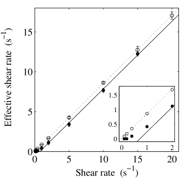
Figure 17: Effective shear rate in the 75 % emulsion ($\bullet$) and in the 20 % emulsion ($\circ$) vs. imposed shear rate. The solid line is the best linear fit of the 75 % data for $\dot{\gamma}\geq 1$ s^-1: $\dot{\gamma}_{\hbox{\rm\scriptsize eff}}=0.85\,\dot{\gamma}-0.61$. The dotted line is the best linear fit of the 20 % data: $\dot{\gamma}_{\hbox{\rm\scriptsize eff}}=0.85\,\dot{\gamma}+0.005$. Inset: blow-up of the low shear regime.

5.2.2 Global flow curve(s)

In the particular case of the concentrated system, it is interesting to compare the classical rheological data $\sigma(\dot{\gamma})$ to the “effective flow curve” $\sigma(\dot{\gamma}_{\hbox{\rm\scriptsize eff}})$ that can be estimated from the local velocity measurements.

Classical steady-state flow measurements were carried out using both a cone-and-plate geometry with striated surfaces (cone angle $2^{\circ}$ and radius 20 mm) and the Couette cell with smooth walls used throughout this study. The emulsion sample was the same as the one used for the velocity profile measurements. Striated surfaces are supposed to minimize wall slip whereas the measurements obtained with the smooth walls lead to the values of $\sigma$ and $\dot{\gamma}$ used up to now.

A constant stress is applied on the sample for ten minutes and the steady-state shear rate is recorded. The flow curves are obtained point by point from the lowest stress upwards. We checked that measurements from the highest stress downwards give the same results. The two steady-state flow curves $\sigma(\dot{\gamma})$ obtained for the concentrated emulsion are compared on logarithmic scales in Fig. 18. The two curves are clearly different. If one considers only the measurements obtained with the Couette geometry, it is not obvious whether the emulsion has a yield stress or not. Indeed, the yield stress inferred from this data set is very small: $\sigma_{\scriptscriptstyle 0}\approx 4$ Pa. On the other hand, measurements obtained with the striated cone-and-plate geometry clearly present a yield stress of about 70 Pa.

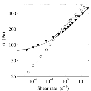
Figure 18: Rheological flow curves $\sigma$ vs. $\dot{\gamma}$ for the 75 % emulsion measured in a striated cone-and-plate geometry ($\blacktriangledown$) and in the Plexiglas Couette cell with smooth walls and $e=3$ mm ($\circ$). The solid line is $\sigma=70+120\,\dot{\gamma}^{0.4}$ and the equation of the dotted line is $\sigma=4+220\,\dot{\gamma}^{0.4}$.

However, even when using striated surfaces, global rheological measurements may still be affected by small slippage or by fracture behaviour at shear rates close to the yield point Mason:1996a . The determination of a precise value for the yield stress is thus difficult with standard rheological tools. A way around the problem is to measure the local velocity and plot the shear stress as a function of the effective shear rate $\dot{\gamma}_{\hbox{\rm\scriptsize eff}}$ in the sample.

5.2.3 Local flow curve

As seen in Fig. 19 where the “effective flow curve” $\sigma(\dot{\gamma}_{\hbox{\rm\scriptsize eff}})$ is compared to the global rheological data obtained in the Couette cell, $\sigma(\dot{\gamma}_{\hbox{\rm\scriptsize eff}})$ yields yet another flow curve, different from the curves of Fig. 18. Now, the two points where the emulsion does not flow lie on the axis $\dot{\gamma}=0$ and the data corresponding to $\dot{\gamma}\geq 0.4$ s^-1 seem to point to a higher value of the yield stress around 90 Pa. As we shall see below, the present data do not allow us to draw definite conclusions about the value of the yield stress nor even about the existence of a simple analytic flow curve for the concentrated emulsion.

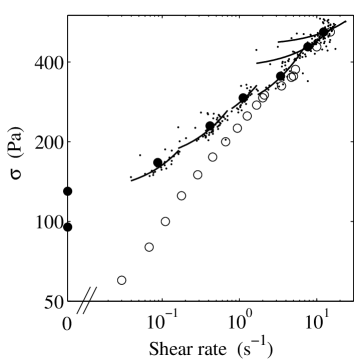
Figure 19: The “effective flow curve” $\sigma$ vs. $\dot{\gamma}_{\hbox{\rm\scriptsize eff}}$ ($\bullet$) and the “local flow curve” $\sigma(x)$ vs. $\dot{\gamma}(x)$ (dots) for the 75 % emulsion compared to the rheological data obtained in the Plexiglas Couette cell ($\circ$). The solid segments are linear fits of the local data $\sigma(x)$ vs. $\dot{\gamma}(x)$.

Since the velocity profiles are curved, one may argue that plotting the effective shear rate $\dot{\gamma}_{\hbox{\rm\scriptsize eff}}$ against the shear stress given by the rheometer is not such an accurate estimate of the flow curve. However, using local measurements, one can go one step further and estimate the local shear rate $\dot{\gamma}(x)$ by differentiating the velocity profile $v(x)$ according to:

$$\dot{\gamma}(x)=-(R_{\scriptscriptstyle 1}+x)\,\frac{\partial}{\partial x}\left(\frac{v(x)}{R_{\scriptscriptstyle 1}+x}\right)\,.$$ (8)

This was done directly on the raw velocity data with a first-order approximation for the derivative: $\partial v/\partial x\approx\delta v/\delta x=(v(x+\delta x)-v(x))/\delta x$. The minus sign in Eq. (8) accounts for the orientation of the $x$ axis along decreasing velocities.

Moreover, if the flow is stationary and the sample does not present any fracture, then $\nabla\sigma=0$ and the local shear stress reads:

$$\sigma(x)=\sigma_{\scriptscriptstyle 1}\left(\frac{R_{\scriptscriptstyle 1}}{R_{\scriptscriptstyle 1}+x}\right)^{2}\,,$$ (9)

where $R_{\scriptscriptstyle 1}$ is the radius of the rotor and $\sigma_{\scriptscriptstyle 1}=\sigma(x=0)$ the shear stress applied by the rheometer on the rotor. Note that this equation was already implicitely used at the walls when writing Eq. (6). For each velocity profile and for each value of $x$, the point $(\dot{\gamma}(x),\sigma(x))$ obtained by Eqs. (8) and (9) is plotted in Fig. 19.

We check that the data $(\dot{\gamma}(x),\sigma(x))$ are scattered around the effective flow curve $\sigma(\dot{\gamma}_{\hbox{\rm\scriptsize eff}})$. The dispersion seen in this “local flow curve” $(\dot{\gamma}(x),\sigma(x))$ mainly arises from the experimental estimation of the derivative in Eq. (8). For each shear rate, each cluster of points $(\dot{\gamma}(x),\sigma(x))$ was fitted by a straight line. The resulting segments are plotted in logarithmic scales in Fig. 19. It can be seen that $(\dot{\gamma}_{\hbox{\rm\scriptsize eff}},\sigma)$ always fall close to these first order approximations of the local flow curve. Note that due to the inhomogeneity of the stress in the Couette cell, the shear rates explored locally continuously cover the whole range 0.03 s^-1–20 s^-1.

However, a jump in the local behaviour can be clearly identified between $\dot{\gamma}=1$ s^-1 and $\dot{\gamma}=5$ s^-1 and the local flow curve does not appear to be continuous at larger shear rates. Thus, within the precision of our data, it looks as though the local flow behaviour differs from one imposed shear rate to another, at least for $\dot{\gamma}\geq 1$ s^-1. These results indicate that the very notion of a simple analytic flow curve may become questionable at high shear rates for our concentrated emulsion. In the next paragraph, we try to make this point clearer by focussing on the precise shape of the velocity profiles.

5.3 Trying to account for the curvature of the velocity profiles

5.3.1 Testing the flow behaviour $\sigma=A\dot{\gamma}^{n}$

Using MRI, Coussot et al. Coussot:2002 found that above some critical stress $\sigma_{c}$, the velocity profiles of various flowing concentrated materials were well described by a local power-law behaviour:

$$\dot{\gamma}(x) = 0\,\,\,\hbox{\rm for}\,\,\,\sigma<\sigma_{c}\,,$$ (10)

$$\sigma(x) = A\,\dot{\gamma}(x)^{n}\,\,\,\hbox{\rm for}\,\,\,\sigma\geq\sigma_{c}\,.$$ (11)

Those two equations describe a flow behaviour with two separate branches. Equation (10) represents the jammed state and holds below the yield point $\sigma_{c}$. Equation (11) corresponds to a power-law fluid. The case $n=1$ and $\sigma_{c}=0$ corresponds to the case of a Newtonian fluid ($A$ is then the usual viscosity $\eta$). $n<1$ (resp. $n>1$) means that the fluid is shear-thinning (resp. shear-thickening). This exponent $n$ controls the curvature of the velocity profiles $v(x)$. In light of the results of Ref. Coussot:2002 , we wanted to test whether Eq. (11) was able to account for the shape of our velocity profiles when the emulsion flows i.e. for $\dot{\gamma}>0.2$ s^-1.

Theoretical velocity profiles.

Using Eqs. (8), (9) and (11), it is straightforward to calculate the flow profile above the yield point:

$$v(x) =v_{\scriptscriptstyle 2}\,\frac{R_{\scriptscriptstyle 1}+x}{R_{\scriptscriptstyle 2}}\,+$$

$$(R_{\scriptscriptstyle 1}+x)\,\frac{n}{2}\left(\frac{\sigma_{\scriptscriptstyle 1}}{A}\left(\frac{R_{\scriptscriptstyle 1}}{R_{\scriptscriptstyle 2}}\right)^{2}\right)^{1/n}\left(\left(\frac{R_{\scriptscriptstyle 2}}{R_{\scriptscriptstyle 1}+x}\right)^{2/n}-1\right)\,,$$ (12)

and the velocities of the emulsion at the two walls are linked by:

$$v_{\scriptscriptstyle 1}=v_{\scriptscriptstyle 2}\,\frac{R_{\scriptscriptstyle 1}}{R_{\scriptscriptstyle 2}}+R_{\scriptscriptstyle 1}\,\frac{n}{2}\left(\frac{\sigma_{\scriptscriptstyle 1}}{A}\left(\frac{R_{\scriptscriptstyle 1}}{R_{\scriptscriptstyle 2}}\right)^{2}\right)^{1/n}\left(\left(\frac{R_{\scriptscriptstyle 2}}{R_{\scriptscriptstyle 1}}\right)^{2/n}-1\right)\,.$$ (13)

As before, $\sigma_{\scriptscriptstyle 1}$ denotes the shear stress at the moving inner wall: $\sigma_{\scriptscriptstyle 1}=\sigma(x=0)$. Using Eqs. (12), (13), and the definition of Eq. (4), the normalized flow profile is given by:

$$v_{n}(x)\approx\left(1+\frac{x}{R_{\scriptscriptstyle 1}}\right)\,\frac{\left(\frac{R_{\scriptscriptstyle 2}}{R_{\scriptscriptstyle 1}+x}\right)^{2/n}-1}{\left(\frac{R_{\scriptscriptstyle 2}}{R_{\scriptscriptstyle 1}}\right)^{2/n}-1}\,.$$ (14)

The previous approximation results from the assumption that $v_{\scriptscriptstyle 1}/R_{\scriptscriptstyle 2}\ll\dot{\gamma}(x)$ everywhere in the cell gap. Since $v_{\scriptscriptstyle 1}\lesssim v_{\scriptscriptstyle 0}$, $\dot{\gamma}(x)\lesssim v_{\scriptscriptstyle 0}/e$, and $R_{\scriptscriptstyle 2}\simeq 10\,e$, Eq. (14) holds with an accuracy that is always better than the experimental uncertainty of about 5 %.

Experimental determination of the exponent $n$.

Equation (14) shows that in the framework of Eq. (11), focussing on $v_{n}(x)$ allows us to remove the contributions of both the slip velocity $v_{\scriptscriptstyle 2}$ and the prefactor $A$ to the velocity profiles, so that the only free parameter is $n$. Figure 20(a) presents theoretical profiles obtained with Eq. (14) for $R_{\scriptscriptstyle 1}=22$ mm, $R_{\scriptscriptstyle 2}=25$ mm, and values of $n$ ranging from 0.2 to 1. The inset shows that velocity profiles can hardly be distinguished from one another when $0.6\leq n\leq 1$. In Fig. 20(b), we plotted the master curve $<v_{n}(x)>$ found for the concentrated emulsion (inset of Fig. 13) together with theoretical profiles for $n=0.3$, 0.4, and 0.5 given by Eq. (14). The experimental data and their error bars fall between the theoretical profiles with $n=0.3$ and $n=0.5$ so that we have $n=0.4\pm 0.1$ in the case of the concentrated emulsion. This value of $n$ is compatible with both the model of Princen Princen:1989 that predicts an exponent $n=1/2$ and that of Berthier et al. Berthier:2001 which yields $n=1/3$ close to the glass transition in soft materials.

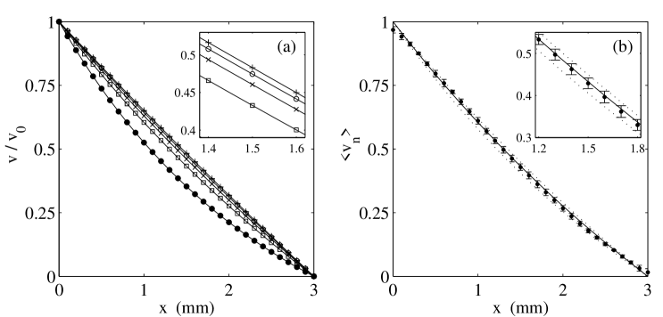
Figure 20: (a) Theoretical velocity profiles obtained with Eq. (14) for $n=0.2$ ($\bullet$), 0.4 ($\Box$), 0.6 ($\times$), 0.8 ($\circ$), and 1 ($+$). Inset: blow-up of the middle of the gap. (b) Average normalized profiles for the 75 % emulsion $<v_{n}>$ ($\bullet$) and the non-Newtonian predictions of Eq. (14) with $n=0.3$ (lower dotted line), $n=0.4$ (solide line), and $n=0.5$ (upper dotted line). Inset: blow-up of the middle of the gap.

When performed on the dilute emulsion, the same analysis yields $n=1\pm 0.1$. In this case, the very small curvature of $v_{n}(x)$ due to the variation of $\sigma(x)$ across the gap cannot be detected and the Newtonian profile is undistinguishable from a straight line, at least in a Couette cell with $R_{\scriptscriptstyle 1}=22$ mm and $e=3$ mm. On the other hand, when the fluid is shear-thinning enough, say when $n<0.6$, the effect of the shear stress non-uniformity is enhanced and curvature becomes quantitatively measurable even in a Couette cell with a rather small gap. All the velocity profiles obtained with the concentrated emulsion are consistent with a single value of $n=0.4\pm 0.1$ and more experiments, perhaps in wider gaps, could help discriminate between $n=1/3$ and $n=1/2$. However, for the model to be fully applicable, one still has to check that Eq. (11) holds for a single value of the parameter $A$ over the whole range of investigated shear rates.

Experimental determination of the parameter $A$ and failure of the model.

Once $n$ is known, it is possible to estimate the prefactor $A$ from our experimental data. More precisely, the data in Figs. 4–7 and 10–12 were fitted using a least-square algorithm by:

$$v(x)=B\,\frac{R_{\scriptscriptstyle 1}+x}{R_{\scriptscriptstyle 2}}+C\,(R_{\scriptscriptstyle 1}+x)\left(\left(\frac{R_{\scriptscriptstyle 2}}{R_{\scriptscriptstyle 1}+x}\right)^{2/n}-1\right)\,,$$ (15)

where $B$ and $C$ are free parameters and $n$ was fixed to $n=1$ for the 20 % emulsion and $n=0.4$ for the 75 % emulsion. The best fits are plotted in solid lines in the corresponding figures. In all cases, those fits describe the experimental data very closely. Note that for the concentrated emulsion at $\dot{\gamma}=0.1$ s^-1 and $0.2$ s^-1 (Fig. 9), the data were fitted by straight lines since the emulsion undergoes solid-body rotation in this low shear regime.

Moreover, if Eq. (12) holds, one expects:

$$B=v_{\scriptscriptstyle 2}\,\,\,\hbox{\rm and}\,\,\,C=\frac{n}{2}\left(\frac{\sigma_{\scriptscriptstyle 1}}{A}\left(\frac{R_{\scriptscriptstyle 1}}{R_{\scriptscriptstyle 2}}\right)^{2}\right)^{1/n}\,.$$ (16)

Hence, if the power-law behaviour of Eq. (11) is verified, one should have:

$$D\,\widehat{=}\,{\left(\frac{R_{\scriptscriptstyle 2}}{R_{\scriptscriptstyle 1}}\right)}^{2}{\left(\frac{2C}{n}\right)}^{n}=\frac{\sigma_{\scriptscriptstyle 1}}{A}\,.$$ (17)

Thus, an important self-consistency check of the model can be performed by plotting $D$ against the shear stress at the rotor $\sigma_{\scriptscriptstyle 1}$. As shown in Fig. 21(a), the data for the dilute emulsion are very well fitted by $D=\sigma_{\scriptscriptstyle 1}/A$ with $A\approx 0.042$. This is consistent with the Newtonian behaviour of the 20 % emulsion and with the value found for its viscosity from rheological measurements when corrected for wall slip ($\eta=0.043$ Pa.s).

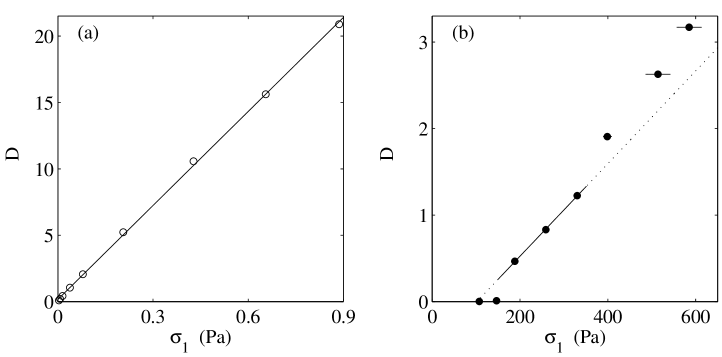
Figure 21: The parameter $D$ vs. $\sigma$ (see text). (a) For the 20 % emulsion ($\circ$), the best linear fit yields $A=0.042$. (b) For the 75 % emulsion ($\bullet$), the best linear fit for $150<\sigma_{\scriptscriptstyle 1}<350$ Pa (i.e. $0.4\leq\dot{\gamma}\leq 1$ s^-1) does not go to zero when $\sigma_{\scriptscriptstyle 1}\to 0$.

As for the concentrated emulsion, the behaviour is quite different. Figure 21(b) shows that the parameter $D$ no longer behaves linearly with $\sigma_{\scriptscriptstyle 1}$ and, more important, that $D$ no longer goes to zero when $\sigma_{\scriptscriptstyle 1}$ goes to zero. Instead, $D(\sigma_{\scriptscriptstyle 1})$ intersects the axis $D=0$ at a shear stress $\sigma_{\scriptscriptstyle 1}$ of about 100 Pa which corresponds to $\sigma\approx 90$ Pa (using Eq. (6)). This means that, when calculated by $A=\sigma_{\scriptscriptstyle 1}/D$ according to Eq. (17), $A$ varies from 407 to 185 when $\dot{\gamma}$ increases from 0.4 to 15 s^-1. This strong variation of $A$ with $\sigma$ shows that, even though the individual fits by Eq. (15) are all very good, our data are not compatible with the flow behaviour given by Eq. (11) with a single constant $A$. In particular, Eq. (11) may well hold locally and for a single value of $n$, but $A$ has to be allowed to vary with $\sigma$ in order to account for the experimental data. Thus, in the case of our concentrated emulsion, the local model used in Ref. Coussot:2002 fails to describe the whole range of investigated shear stresses with a single exponent $n=0.4$ and a single value of $A$.

5.3.2 Influence of a yield stress

In the case of the concentrated emulsion, it is very tempting to interpret the particular value $\sigma_{\scriptscriptstyle 0}$ of the stress where $D(\sigma_{\scriptscriptstyle 0})=0$ as a “yield stress”. However, if we assume the following local behaviour based on the Herschel-Bulkley equation:

$$\sigma(x)=\sigma_{\scriptscriptstyle 0}+A\,\dot{\gamma}(x)^{n}\,\,\,\hbox{\rm for}\,\,\,\sigma\geq\sigma_{\scriptscriptstyle 0}\,,$$ (18)

the above analysis of the velocity profiles is no longer valid. Indeed, if Eq. (18) holds and if $n\neq 1$, the velocity $v(x)$ is no longer easily integrable from Eqs. (8) and (9). Instead, for $n\neq 1$, one gets:

$$\frac{v(x)}{R_{\scriptscriptstyle 1}+x}=\frac{v_{\scriptscriptstyle 1}}{R_{\scriptscriptstyle 1}}+\int_{R_{\scriptscriptstyle 1}}^{R_{\scriptscriptstyle 1}+x}{\,\frac{\hbox{\rm d}r}{r}\left[\frac{\sigma\left(\frac{R_{\scriptscriptstyle 1}}{r}\right)^{2}-\sigma_{\scriptscriptstyle 0}}{A}\right]^{1/n}\,.}$$ (19)

Note that we can rule out the case $n=1$ for two reasons: (i) although they do not allow for a reliable measurement of $\sigma_{\scriptscriptstyle 0}$, rheological data indicate a power-law behaviour with $n\approx 0.4$ at large $\dot{\gamma}$ (see Fig. 18), and (ii) $n=1$ leads to velocity profiles whose curvatures varie strongly from a logarithmic shape close to $\sigma_{\scriptscriptstyle 0}$ to an almost linear shape when $\sigma\gg\sigma_{\scriptscriptstyle 0}$, whereas the curvature of our experimental profiles does not vary noticeably (see Fig. 13).

We integrated Eq. (19) numerically and looked for a set of parameters $v_{\scriptscriptstyle 1}$, $\sigma_{\scriptscriptstyle 0}$, $A$, and $n$ that would describe all the different profiles. Since $v_{\scriptscriptstyle 1}$ corresponds to slip at the rotor, the values $v_{\scriptscriptstyle 1}(\sigma)$ found earlier in this paper were forced into the equation. We also set $n=0.4$ because this value seems to describe correctly the shear-thinning behaviour of our emulsion (see Figs. 18 and 20(b)). With only two free parameters $\sigma_{\scriptscriptstyle 0}$ and $A$, we were then able to fit the velocity profiles very closely so that the fits were undistinguishable from those obtained previously with Eq. (15). However, once again, we could not find a single set of parameters to fit all the velocity profiles. $A$ and $\sigma_{\scriptscriptstyle 0}$ had to be allowed to vary significantly with $\sigma$ so that the whole range of investigated shear rates could be accounted for.

Due to the restricted amount of data and to the experimental uncertainty, it was not reasonable to allow one more free parameter in the fits, namely to allow $n$ to vary. In that case, almost any value of $n$ between 0.1 and 0.7 could be obtained by tuning $A$ and $\sigma_{\scriptscriptstyle 0}$. Indeed, in the frawework of Eqs. (18) and (19), the curvature of $v(x)$ is not only controlled by $n$ but is also very sensitive to $\sigma_{\scriptscriptstyle 0}$. However, if we restrict the analysis to the range $0.2<\dot{\gamma}<5$ s^-1 where $D(\sigma_{\scriptscriptstyle 1})$ appears as very linear on Fig. 21(b), we showed that $n=0.4$ and $\sigma_{\scriptscriptstyle 0}=90\pm 10$ Pa were reasonable parameters for this range of applied shear rates. Note that this range of shear rates corresponds to the domain where the local flow curve of Fig. 19 seems the most continuous.

5.3.3 Existence of a global flow curve

The above problems encountered during the analysis of the individual velocity profiles raise the question of the existence of a global flow curve for the concentrated system. Indeed, it seems that simple approaches based on Eqs. (11) or (18) fail to describe our experimental data for the 75 % emulsion with a single set of parameters. The fact that the curvature of the individual profiles may be nicely fitted in terms of one of these two equations means that those flow behaviours may be representative of the fluid at a local level for a given shear rate. However, except on a small range of $\dot{\gamma}$, this kind of simple flow behaviour does not hold globally: the parameters have to be adjusted from one shear rate to another. This result is in agreement with measurements by Mason et al. Mason:1996a who report that for emulsions of droplet size 0.25 $\mu$m and concentrated above 65 %, $\sigma(\dot{\gamma})$ deviates from a power law at high $\dot{\gamma}$.

Thus, our results would lead to a general picture of a sheared concentrated emulsion as a material whose flow behaviour changes with the imposed stress due to subtle changes in its micro-structure:

$$\sigma(x)=\sigma_{\scriptscriptstyle 0}(\sigma)+A(\sigma)\,\dot{\gamma}(x)^{n(\sigma)}\,.$$ (20)

Indeed, even though we checked that the mean radius of the oil droplets did not change during our experiments, the parameters controlling the flow behaviour such as the shear-thinning exponent $n$ may depend on the compression state of the droplets or on their precise shape or even on the sample history.

6 Discussion and conclusions

In this paper, we presented local velocity measurements in a dilute and in a concentrated emulsion using heterodyne DLS. In both systems, we found significant slippage. We have shown that the corrections for wall slip usually introduced in rheology are valid for the concentrated emulsion. However, in the dilute emulsion, inertial effects may come into play and complicate the analysis so that direct estimate of slip velocities are required.

Once wall slip is measured, we can access interesting local rheological information. We found that the dilute emulsion has a Newtonian behaviour and that the concentrated system is shear-thinning with an exponent close to 0.4 that accounts well for the curvature of the velocity profiles. It also seems that the behaviour of the concentrated emulsion cannot be described by a single flow curve over the whole range of shear rates that we investigated. This raises the question of the definition of a global flow curve.

We have also shown that for the smallest shear rates at which the concentrated system flows ($0.4\leq\dot{\gamma}\leq 1$ s^-1), the flow behaviour is compatible with a yield-stress fluid with $\sigma_{\scriptscriptstyle 0}\approx 90$ Pa and $n\approx 0.4$. In any case, our results clearly rule out a simple power-law behaviour with a single prefactor $A$ (see Fig. 21(b)). For $\dot{\gamma}\leq 0.2$ s^-1, the emulsion does not flow and behaves like a solid. This shows the existence of two different regimes: one where the system is solid-like and one where the system flows like a yield-stress fluid. Up to the precision of the present data, the two shear rates at which the system is solid-like seem to correspond to shear stresses slightly above $\sigma_{\scriptscriptstyle 0}$ ($\sigma=100$ and 130 Pa, see Fig. 19). This raises important questions about the behaviour of a concentrated emulsion near the transition between the two regimes.

Indeed, recent experiments Coussot:2002 ; Debregeas:2001 and numerical simulations Varnik:2002pp on soft disordered materials have focussed on the local flow properties of yield-stress systems like clay suspensions, industrial gels, emulsions and foams. Such systems were shown to present inhomogeneous flow profiles when sheared close to their yield point: the sample separates between a fluid-like phase near the rotor and a solid-like phase near the fixed wall of a Couette cell. In some cases, the velocity profiles in the fluid phase show a strong curvature very similar to that observed on our measurements in the concentrated emulsion Coussot:2002 . These features seem quite general since they have also been observed in colloidal suspensions and granular pastes Pignon:1996 ; Barentin:2002pp .

Since the first models of soft glassy materials under shear Bouchaud:1995 ; Sollich:1997 and triggered by recent experimental developments on aging and rejuvenation Cloitre:2000 ; Ramos:2001 ; Viasnoff:2002 , intense theoretical effort is currently being spent on the understanding of the yield stress phenomenon Lemaitre:2002 ; Fuchs:2002pp_a ; Fuchs:2002pp_b and on the possible existence of two separate branches in the flow behaviour Derec:2001 ; Berthier:2002pp . In particular, hysteretic effects are expected when the shear stress is controlled and the presence of shear bands is predicted when the shear rate is imposed Picard:2002pp .

So far, we have not been able to show that inhomogeneous flows and/or hysteretic effects take place in the 75 % emulsion when sheared in our small gap geometry ($e=3$ mm for $R_{\scriptscriptstyle 1}=22$ mm). Direct visualization of the emulsion surface as in Refs. Mason:1996a ; Princen:1985 is made impossible by the use of a thermostated cover that prevents evaporation of our samples. Moreover, let us recall that our velocity profiles are obtained in typically 30 minutes. The flow profiles of Fig. 9 showing solid-body rotation may thus miss transient inhomogeneous behaviours that could occur on shorter time scales such as fracture or stick-slip phenomena.

However, none of the velocity profiles presented here seems consistent with a stationary banded flow as described in Refs. Coussot:2002 ; Debregeas:2001 . More experiments around the yield point will be needed to conclude on this issue. In particular, in the framework of the recent theoretical approaches of inhomogeneous flows, the existence of two points above the yield stress where the system behaves like a solid body should lead to inhomogeneous and possibly non-stationary flows in this region. Future experiments will focus on this specific point. We also intend to use high-frequency ultrasound to measure velocity profiles with an increased temporal resolution (0.01–0.1 s) in order to capture transient and possibly non-stationary flows.

- (1) R. G. Larson. The structure and rheology of complex fluids. Oxford University Press, 1999.
- (2) T. G. Mason, J. Bibette, and D. A. Weitz. Yielding and flow of monodisperse emulsions. J. Colloid Interface Sci., 179:439–448, 1996.
- (3) H. A. Barnes. Rheology of emulsions — a review. Colloids and Surfaces A, 91:89–95, 1994.
- (4) P. Coussot, J. S. Raynaud, F. Bertrand, P. Moucheront, J. P. Guilbaud, H. T. Huynh, S. Jarny, and D. Lesueur. Coexistence of liquid and solid phases in flowing soft-glassy materials. Phys. Rev. Lett., 88:218301, 2002.
- (5) J.-B. Salmon, S. Manneville, A. Colin, and B. Pouligny. An optical fiber based interferometer to measure velocity profiles in sheared complex fluids. Submitted to Eur. Phys. J. AP. E-print cond-mat/0211013, 2002.
- (6) T. G. Mason and J. Bibette. Emulsification in viscoelastic media. Phys. Rev. Lett., 77:3481, 1996.
- (7) B. J. Berne and R. Pecora. Dynamic light scattering. Wiley, New York, 1995.
- (8) B. J. Ackerson and N. A. Clark. Dynamic light scattering at low rates of shear. J. Physique, 42:929–936, 1981.
- (9) J. P. Gollub and M. H. Freilich. Optical heterodyne study of the taylor instability in a rotating fluid. Phys. Rev. Lett., 33:1465–1468, 1974.
- (10) H. M. Princen. Rheology of foams and highly concentrated emulsions. ii. experimental study of the yield stress and wall effects for concentrated oil-in-water emulsions. J. Colloid Interface Sci., 105:150–171, 1985.
- (11) H. A. Barnes. A review of the slip (wall depletion) of polymer solutions, emulsions and particle suspensions in viscometers: Its cause, character, and cure. J. Non-Newtonian Fluid Mech., 56:221–251, 1995.
- (12) H. L. Goldsmith and S. G. Mason. The flow of suspensions through tubes. i. single spheres, rods, and discs. J. Colloid Sci., 17:448–476, 1962.
- (13) A. S. Yoshimura and R. K. Prud’homme. Wall slip corrections for couette and parallel disk viscometers. J. Rheol., 32:53–67, 1988.
- (14) T. Kiljański. A method for correction of the wall-slip effect in a couette rheometer. Rheol. Acta, 28:61–64, 1989.
- (15) M. Mooney. Explicit formulas for slip and fluidity. J. Rheol., 2:210–222, 1931.
- (16) H. M. Princen and A. D. Kiss. Rheology of foams and highly concentrated emulsions. iv. an experimental study of the shear viscosity and yield stress of concentrated emulsions. J. Colloid Interface Sci., 128:176–187, 1989.
- (17) L. Berthier, J.-L. Barrat, and J. Kurchan. A two-time-scale, two-temperature scenario for nonlinear rheology. Phys. Rev. E, 61:5464–5472, 2000.
- (18) G. Debrégeas, H. Tabuteau, and J.-M. di Meglio. Deformation and flow of a two-dimensional foam under continuous shear. Phys. Rev. Lett., 87:178305, 2001.
- (19) F. Varnik, L. Bocquet, J.-L. Barrat, and L. Berthier. Shear localization in a model glass. E-print cond-mat/0208485, 2002.
- (20) F. Pignon, A. Magnin, and J.-M. Piau. Thixotropic colloidal suspensions and flow curves with minimum: Identification of flow regimes and rheometric consequences. J. Rheol., 40:573, 1996.
- (21) C. Barentin and B. Pouligny. To be published.
- (22) J.-P. Bouchaud and D. S. Dean. Aging on parisi’s tree. J. Phys. I France, 5:265–286, 1995.
- (23) P. Sollich, F. Lequeux, P. Hébraud, and M. E. Cates. Rheology of soft glassy materials. Phys. Rev. Lett., 78:2020–2023, 1997.
- (24) M. Cloître, R. Borrega, and L. Leibler. Rheological aging and rejuvenation in microgel pastes. Phys. Rev. Lett., 85:4819–4822, 2000.
- (25) L. Ramos and L. Cipelletti. Ultraslow dynamics and stress relaxation in the aging of a soft glassy system. Phys. Rev. Lett., 87:245503, 2001.
- (26) V. Viasnoff and F. Lequeux. Rejuvenation and overaging in a colloidal glass under shear. Phys. Rev. Lett., 89:065701, 2002.
- (27) A. Lemaître. Rearrangements and dilatancy for sheared dense materials. Phys. Rev. Lett., 89:195503, 2002.
- (28) M. Fuchs and M. E. Cates. Theory of nonlinear rheology and yielding of dense colloidal suspensions. E-print cond-mat/0204628, 2002.
- (29) C. B. Holmes, M. Fuchs, and M. E. Cates. Jamming transitions in a mode-coupling model of suspension rheology. E-print cond-mat/0210321, 2002.
- (30) C. Derec, A. Ajdari, and F. Lequeux. Rheology and aging: A simple approach. Eur. Phys. J. E, 4:355–361, 2001.
- (31) L. Berthier. Yield stress, heterogeneities and activated processes in soft glassy materials. E-print cond-mat/0209394, 2002.
- (32) G. Picard, A. Ajdari, L. Bocquet, and F. Lequeux. A simple model for heterogeneous flows of yield stress fluids. E-print cond-mat/0206260, 2002.