Anisotropy in granular media: classical elasticity and directed force chain network

Abstract

A general approach is presented for understanding the stress response function in anisotropic granular layers in two dimensions. The formalism accommodates both classical anisotropic elasticity theory and linear theories of anisotropic directed force chain networks. Perhaps surprisingly, two-peak response functions can occur even for classical, anisotropic elastic materials, such as triangular networks of springs with different stiffnesses. In such cases, the peak widths grow linearly with the height of the layer, contrary to the diffusive spreading found in ‘stress-only’ hyperbolic models. In principle, directed force chain networks can exhibit the two-peak, diffusively spreading response function of hyperbolic models, but all models in a particular class studied here are found to be in the elliptic regime.

I Introduction

The stress response of an assembly of hard, cohesionless grains has been a subject of debate deG ; Savage ; us ; Proc . The dividing line has been mostly between traditional approaches based on elasticity or elastoplasticity theory on one hand, and “stress-only” models on the other which make no reference to a local deformation field but posit (history-dependent) closure relations between components of the stress tensor. The former leads to elliptic partial differential equations for the stresses, for which boundary conditions must be imposed everywhere on the boundary. In contrast, the latter approach often leads to hyperbolic equations us ; Proc . The wave-like behavior of their solutions has been at the origin of a proposed physical mechanism called stress propagation through the bulk a granular material. In an infinite slab geometry, it only requires the specification of boundary conditions on the “top” surface. A family of (linear) closure relations have been shown to account for the pressure dip underneath the apex of a sandpile and stresses in silos us ; Proc . Alternative explanations based on elastoplasticity are found in Cantelaube .

The phenomenological ‘stress-only’ closure relations follow from plausible symmetry arguments, and can be seen as the coarse-grained version of local probabilistic rules for stress transfer pre . However, these relations lack a detailed microscopic derivation that would allow one both to understand their range of validity and to compute the phenomenological parameters from the statistical properties of the packing, except in the case of frictionless grains. In fact, a system of frictionless polydisperse spheres is shown to be isostatic bcc ; Roux ; moukarzel ; Witten , i.e. the number of unknown forces is equal to the number of equations for mechanical equilibrium. If an isostatic system is sufficiently anisotropic, a linear closure relation between stresses can be derived Edwards . Further attempts to obtain the missing equation for stresses from a microscopic approach for different packings are presented in Edwards ; Ball , but these are still somewhat inconclusive. In particular, in the case of a completely isotropic packing, none of the homogeneous linear closure relations is compatible with the rotational symmetry. The idea of ‘grains’ (in the metallurgical sense) and packing defects must be introduced to restore the large scale symmetry.

In order to understand stress distribution on a more fundamental level, we have introduced the mesoscopic concept of the directed force chain network (dfcn) bclo ; ssc , which is motivated by the experimental evidence for filamentary force chains in a wide variety of systems.photo . The “double Y” model has been developed to describe such networks based on simple rules for the splitting and merging of straight force chains. This model leads to a non-linear Boltzmann equation for the probability $P(f,\hat{\bf n},{\bf r})$ of finding a force chain at the spatial point ${\bf r}$ with intensity $f$ in the direction $\hat{\bf n}$.

In a first paper bclo , chain merging (which produces the non-linear terms in the Boltzmann equation) was neglected. An isotropic splitting rule was assumed, corresponding to strongly disordered isotropic granular packings. A pseudo-elastic theory for the stress tensor was derived in which the role of the displacement field is played by a vector field ${\bf J}({\bf r})=\langle\hat{\bf n}f\rangle$ that represents the coarse-grained or ensemble averaged force chain direction. A relation between $\partial_{i}J_{j}$ and the stress tensor exists that is formally equivalent to an isotropic stress-strain relation. The resulting elliptic equations yield a response function with a unique (pseudo-elastic) peak, as observed experimentally in strongly disordered packings Reydellet ; Reydelletbis . Further study showed, however, that the non-linear terms in the Boltzmann equation contain essential physics and cannot be neglected. ssc In fact, for an exactly solvable model with 6 discrete directions for force chains, it was found that the elliptic (pseudo-elastic) behavior of the response function is limited to small depths, and that at sufficiently large depths a crossover occurs to an hyperbolic response – two Gaussian peaks that propagate away and broaden diffusively. Whether this behavior is specific to the model with 6 discrete directions is a subject of current study, and the elliptic or hyperbolic nature of the linearized response around the full solution of the nonlinear Boltzmann equation is an open question.

Following a different route, Goldenberg and Goldhirsch goldhirsch have recently noted that a two-peak response function can be found in classical anisotropic ball-and-spring models. Gay and da Silveira Gay have furthermore given some arguments for the relevance of anisotropic elasticity for the large scale description of granular assemblies of compressible grains that can locally rotate. The two-peak nature of the response function is therefore not, in itself a signature of hyperbolicity, but may occur in elliptic systems that are sufficiently anisotropic. The unambiguous signature of hyperbolic response lies in the scaling of the peak widths with depth, which is linear in generic elliptic systems but diffusive (proportional to the square root of depth) in generic hyperbolic systems. In the linear pseudo-elasticity theories discussed below, the diffusive spreading in hyperbolic systems is not captured; the peaks appear as delta functions that do not spread at all. Deviations from elasticity on small scales and their possible relation with granular media were also discussed in Tanguy .

The aim of this paper is to give a unified account of the shape of the response function for anisotropic systems described either by standard elasticity theory or the pseudo-elastic theory that emerges from an approximate linear treatment of directed force networks. Though there are open questions concerning the self-consistency of the latter, there do appear to be some contexts in which the equations of the pseudo-elasticity theory hold, and they may be especially relevant for systems of intermediate depth (large compared to the disorder length scale but not much larger than the persistence length of force chains).

Very recently, the response functions of two-dimensional granular layers subjected to shear have been determined experimentally geng . Under shear, an anisotropic texture appears and force chains are preferably oriented along an angle of 45 degrees. Within the (pseudo)-elasticity framework presented below, this provides motivation for studying materials characterized by a selected global direction ${\bf N}$.

The paper is organized as follows. In section 2 a general mathematical framework for calculating stress response functions in anisotropic materials. The main results of the paper are then summarized in a ‘phase-diagram’ indicating where ‘one-peak’ or ‘two- peak’ response functions can appear in parameter space. In section 3, we compute the analytic form of the response function for the various phases and show a number of examples of the variety of shapes that are possible, including a brief comment on relation to experimental work. In section 4, we show how the formalism applies to the example of a triangular ball-and-spring network, indicating how spring stiffnesses must be chosen to access all possible regions of the general parameter space. In section 5, a linear anisotropic pseudo-elastic theory is derived from an anisotropic linear directed force chain network model and it is shown that this class of models always lies in the elliptic regime. A conclusion is given in section 6. Algebraic details of several calculations are presented in Appendices.

II Anisotropic elasticity and summary of our results

II.1 General equations for 2D systems with arbitrary
anisotropy

In the following, we present a general framework that covers both classical linear anisotropic elasticity theory LL and a generally anisotropic “pseudo-elasticity” theory, that appears within a linearized treatment of directed force chain networks (see section V). The large scale equations that can be derived in these two approaches are formally identical, although the “pseudo-strain” has a geometric meaning different from the usual strain tensor. For simplicity, we will restrict the discussion to two-dimensional systems.

The most general linear relation between the stress tensor ${\bf\sigma}$ and a symmetric tensor formed from the gradients of a vector field ${\bf u}$ is

$$\sigma_{ij}=\lambda_{ijkl}u_{kl},$$ (1)

where $\sigma_{ij}$ denotes a component of the stress tensor, $u_{ij}\equiv\frac{1}{2}(\partial_{j}u_{i}+\partial_{i}u_{j})$, and summation over repeated indices is implied. In the classical linear theory of elasticity, the vector $u_{i}$ is the displacement field describing the physical deformation of a continuous medium. For usual elastic bodies, the antisymmetric combination $\partial_{j}u_{i}-\partial_{i}u_{j}$ corresponds to a local rotation of the material, which is not allowed here. For granular materials, on the other hand, grains might locally rotate due to the presence of friction. This extension which suggests a continuum description in terms of Cosserat elasticity was recently discussed in Gay . The absence of internal torques requires that the stress tensor is also symmetric. The coefficients $\lambda_{ijkl}$ are material constants and form the elastic modulus tensor. The indices $i,j,k,l$ are equal to $x,z$ where for later purposes $x$ is to be considered as the horizontal coordinate and $z$ a vertical coordinate pointing downward.

Symmetry of both the stress and the strain tensor imply a permutation symmetry within the first and second pair of indices for $\lambda_{ijkl}$, i.e.

$$\lambda_{ijkl}=\lambda_{jikl}=\lambda_{ijlk}=\lambda_{jilk}.$$ (2)

Materials whose behavior is modeled only in terms of equation (1) without any reference to a free energy functional are characterized by an elastic modulus tensor that need not have any symmetries other than equation (2). They are called ‘hypoelastic’ when $u_{ij}$ corresponds to a real strain tensor truesdell . In hyperelastic materials, on the other hand, the existence of quadratic free energy functional

$$F=\frac{1}{2}\lambda_{ijkl}u_{ij}u_{kl}$$ (3)

gives an additional symmetry under exchange of the first and second pair of indices, i.e.

$$\lambda_{ijkl}=\lambda_{klij}.$$ (4)

In the “pseudo-elasticity” theory, the vector $u_{i}$ will be a novel geometric quantity (see below), and the resulting tensor $u_{ij}$ will be called a pseudo-elastic strain tensor. This tensor is still symmetric, as explained in section V, but the above additional symmetry is in general not present.

We wish to construct general solutions of the equilibrium equations

$$\partial_{i}\sigma_{ij}=0.$$ (5)

In order to close the problem for the stress tensor, a supplementary condition is needed which is the condition of compatibility,

$$\partial_{z}^{2}u_{xx}+\partial_{x}^{2}u_{zz}-2\partial_{x}\partial_{z}u_{xz}=0,$$ (6)

resulting simply from the fact that the tensor $u_{ij}$ is built with the derivatives of a vector $u_{i}$. This relation does not depend on a specific interpretation of the tensor in terms of real deformations.

The entries of the stress and strain tensors can be arranged in vector form, i.e. ${\bf\Sigma}=(\sigma_{xx},\sigma_{zz},\sigma_{xz})^{T}$ and ${\bf U}=(u_{xx},u_{zz},u_{xz})^{T}$, giving a matrix representation of the elastic modulus tensor,

$${\bf\Sigma}={\Lambda}\,{\bf U},$$ (7)

where

$${\Lambda}=\left(\begin{array}[]{ccc}\lambda_{xxxx}&\lambda_{xxzz}&2\lambda_{xxxz}\\ \lambda_{zzxx}&\lambda_{zzzz}&2\lambda_{zzxz}\\ \lambda_{xzxx}&\lambda_{xzzz}&2\lambda_{xzxz}\end{array}\right).$$ (11)

The factors of $2$ are due to the symmetry under exchange of the last 2 indices of $\lambda_{ijkl}$ and $u_{kl}$. Now, we want to express the compatibility relation in terms of the stress tensor, so we need to express ${\bf U}$ in terms of ${\bf\Sigma}$, i.e.

$${\bf U}={\cal B}\,{\bf\Sigma},$$ (12)

where ${\cal B}=(B_{ij})={\Lambda}^{-1}$. Then equation (6) for an anisotropic medium is rewritten as follows

$$B_{1j}\partial_{z}^{2}\Sigma_{j}+B_{2j}\partial_{x}^{2}\Sigma_{j}-2B_{3j}\partial_{x}\partial_{z}\Sigma_{j}=0.$$ (13)

For an isotropic medium, $B_{11}=B_{22}$, $B_{21}=B_{12}$, $B_{3i}=B_{i3}=0$, for $i=1,2$, thus the equation reduces to $\Delta(\sigma_{xx}+\sigma_{zz})=0$.

In the following, we will look for solutions of the form $\sigma_{ij}\propto e^{iqx+i\omega z}$. In this case, equation (13), together with the conditions of mechanical equilibrium (5), can be rewritten in matrix form :

$${\cal A}(q,\omega){\bf\Sigma}=0.$$ (14)

A non-trivial solution occurs if $\det({\cal A}(q,\omega))=0$, which leads to a certain dispersion relation of the form $\omega(q)=Xq$ where $X$ obeys the following equation:

$$\frac{B_{22}}{B_{11}}-\frac{B_{23}+2B_{32}}{B_{11}}X+\frac{2B_{33}+B_{21}+B_{12}}{B_{11}}X^{2}-\frac{B_{13}+2B_{31}}{B_{11}}X^{3}+X^{4}=0.$$ (15)

Depending on whether the roots $X$ are real or complex, the response function will be qualitatively different:

• Complex roots, corresponding to elliptic equations for the stress, appear within the classical theory of anisotropic elasticity. The fact that the roots are complex follows from the positivity of the free energy fichera .

• Purely real roots can occur in the context of directed force chain networks considered below. The existence of at least one purely real root of the dispersion relation classifies the problem at hand as ‘hyperbolic’ fichera .

II.2 The case of uniaxial symmetry

Let us consider the case of uniaxial anisotropy and choose $x$ and $z$ to be along the principal axes of anisotropy. Then only $\lambda_{ijkl}$ with even numbers of equal indices is nonzero. Due to the symmetry (2) of $\lambda_{ijkl}$, this leaves one in general with 5 different constants. The matrix $\Lambda$ takes the form

$$\Lambda_{\dagger}=\left(\begin{array}[]{ccc}a&c&0\\ c^{\prime}&b&0\\ 0&0&d\end{array}\right).$$ (19)

We denote it with a dagger to indicate that it corresponds to a material with a vertical uniaxial symmetry. An alternative parametrization of $\Lambda_{\dagger}$, standard in elasticity theory, is

$$\Lambda_{\dagger}=\frac{1}{1-\nu_{x}\nu_{z}}\left(\begin{array}[]{ccc}E_{x}&\nu_{z}E_{x}&0\\ \nu_{x}E_{z}&E_{z}&0\\ 0&0&(1-\nu_{x}\nu_{z})G\end{array}\right),$$ (20)

where $E_{x,z}$ and $G$ are the Young and shear moduli respectively, and $\nu_{x,z}$ the Poisson ratios. Note that the present form includes a linear elasticity theory without a free energy functional. The classical theory is recovered with the extra symmetry $c^{\prime}=c$. In this case, $E_{x}$, $E_{z}$, $\nu_{x}$ and $\nu_{z}$ are not independent, satisfying the relation $\frac{E_{z}}{E_{x}}=\frac{\nu_{z}}{\nu_{x}}$. Together with $G$, we are thus left with four independent constants.

In classical elasticity theory for a uniaxial system, the stress-strain relation is derivable from an energy density of the form

$$F=\frac{1}{2}\left[au_{xx}^{2}+bu_{zz}^{2}+2cu_{xx}u_{zz}+2du_{xz}^{2}\right],$$ (21)

The material described is stable under deformations if and only if $F$ is positive definite for any strain, which requires

$$a>0;\quad b>0;\quad d>0;\quad\mbox{and}\quad ab-c^{2}>0.$$ (22)

Or, equivalently,

$$\nu_{x}\nu_{z}<1;\quad E_{x}>0;\quad E_{z}>0;\quad\mbox{and}\quad G>0.$$ (23)

An elastic material that is permitted to reversibly deform must obey these constraints, but they do not apply to materials for which there is no well-defined free energy quadratic in the strains. We speak of such materials as being described by coefficients that lie outside the “classical stability” range.

The compatibility condition (6) expressed in terms of the stress tensor reads:

$$b\partial^{2}_{z}\sigma_{xx}-c\partial^{2}_{z}\sigma_{zz}-c^{\prime}\partial^{2}_{x}\sigma_{xx}+a\partial^{2}_{x}\sigma_{zz}-2\frac{\det\Lambda}{d^{2}}\partial_{x}\partial_{z}\sigma_{xz}=0$$ (24)

Combining this relation with the two equilibrium conditions of equation (5),

$$\partial_{z}\sigma_{zz}+\partial_{x}\sigma_{xz} = 0,$$ (25)

$$\partial_{z}\sigma_{xz}+\partial_{x}\sigma_{xx} = 0,$$ (26)

we obtain, for any one of the components of the stress tensor:

$$\left(\partial^{4}_{z}+t\partial^{4}_{x}+2r\partial^{2}_{x}\partial^{2}_{z}\right)\sigma_{ij}=0,$$ (27)

where the coefficients $t$ and $r$ are given by

$$t = \frac{a}{b}=\frac{E_{x}}{E_{z}},$$

$$r = \frac{ab-cc^{\prime}-\frac{1}{2}d(c+c^{\prime})}{bd}=\frac{1}{2}E_{x}\left(\frac{2}{G}-\frac{\nu_{z}}{E_{z}}-\frac{\nu_{x}}{E_{x}}\right).$$ (28)

Expanding the stresses in Fourier modes, it is easy to see that the solutions of the equations (25-27) are of the form

$$\sigma_{zz} = \int_{-\infty}^{+\infty}\!\!\!\!\!\!\!\!\!dq\,\sum_{k}a_{k}(q)\,e^{iqx+iX_{k}qz},$$ (29)

$$\sigma_{xz} = C_{xz}-\int_{-\infty}^{+\infty}\!\!\!\!\!\!\!\!\!dq\,\sum_{k}a_{k}(q)\,X_{k}\,e^{iqx+iX_{k}qz},$$ (30)

$$\sigma_{xx} = C_{xx}+\int_{-\infty}^{+\infty}\!\!\!\!\!\!\!\!\!dq\,\sum_{k}a_{k}(q)\,X_{k}^{2}\,e^{iqx+iX_{k}qz},$$ (31)

where $C_{xx}$ and $C_{xz}$ are constants. From equation (27) we see that the $X_{k}$ are the roots of the following quartic equation

$$X^{4}+2rX^{2}+t=0,$$ (32)

a special case of equation (15). There are four solutions:

$$X=\pm\sqrt{-r\pm\sqrt{r^{2}-t}}.$$ (33)

Hence the index $k$ runs from $1$ to $4$. The four functions $a_{k}(q)$ and the constants $C_{xx}$ and $C_{xz}$ must be determined by the boundary conditions, as shown in section III and Appendix B.

We see that only two combinations, $r$ and $t$, of the 5 elastic constants will determine the structure of the response function in anisotropic materials.

II.3 Main results of this paper

We show in figure 1 the various ‘phases’ in the $r$-$t$ plane corresponding to different shapes of the response function, as obtained from the calculation presented in section III below.

The line $t=r^{2}$, for $r<0$, separates the hyperbolic and the elliptic regions. For $t>r^{2}$ (region I), the above roots $X_{k}$ are complex and we write:

$$X_{1}=-X_{4}=\beta-i\alpha,$$ (34)

$$X_{2}=-X_{3}=-\beta-i\alpha,$$ (35)

where $\alpha$ and $\beta$ are positive real numbers. When $t<r^{2}$, $r>0$ (region II), one the other hand, the roots $X_{k}$ are purely imaginary and one has:

$$X_{1}=-X_{4}=-i\alpha_{1},$$ (36)

$$X_{2}=-X_{3}=-i\alpha_{2},$$ (37)

where $\alpha_{1}$ and $\alpha_{2}$ are positive real numbers.

Note that the isotropic limit corresponds to the point $r=1,\,t=1$. As we show in detail in section III, the elliptic region contains a subregion $r<0$, $t>r^{2}$, where the response function has a two peak structure with peak widths growing linearly with depth. As one approaches the line $t=r^{2}$, the two peaks become narrower and narrower, finally becoming two delta-function peaks exactly on the transition line. Below the transition, there is a hyperbolic regime (region III in figure 1) where the response consists of four delta-function peaks.

The parameter range $t<0$, labeled “mixed” in figure 1, gives rise to a third type of behavior of the response function due to the fact that there are two real roots and two imaginary roots. It may only appear in the non-stable pseudo-elastic case, and gives superposition of a hyperbolic two delta peak response function and a single-peka classically elastic response function. For the particular model for the DFCN discussed below, the range $t<0$ does not occur. Hence this case is not pursued any further here.

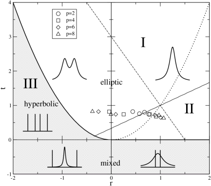
Figure 1: $(r,t)$ phase diagram characterizing the qualitative nature of the stress profiles. The shaded region corresponds to hyperbolic and “mixed” equations for stresses whereas the unshaded region allows for elliptic equations. The hyperbolic region is bounded above by the line $t=r^{2}$, separating it from the elliptic region. In the elliptic region, a double peak stress profile is found in the whole region $r<0$. The solid and dashed straight lines are the trajectories for the triangular spring network studied in section IV, for horizontal and vertical orientation of one of the springs, respectively. The symbols correspond to the solutions of the anisotropic linear dfcn model for various values of the anisotropic scattering parameter $p$, see section V.

We discuss below some particular trajectories in the $r$-$t$ plane (see sections IV and V). One corresponds to simple, anisotropic, triangular networks of springs, that lead on large scales to classical anisotropic elasticity with parameters on the plain and dotted straight lines, corresponding to two orientations of the lattice (see figure 10). Both trajectories meet at the point $(1,1)$ corresponding to an isotropic medium where all springs have the same stiffness. Moreover, both trajectories cross the region $r<0$ and thus allow for two peak response functions. Inclusion of three-body forces permits spring networks with $(r,t)$ anywhere in region I or II (see section IV).

We have also computed $r$ and $t$ for the linear dfcn model, for a particular model for scattering where the degree of anisotropy is tuned in terms of a parameter $p$ (see section V). The results are shown as symbols, and appear to always lie in the elliptic region. As in the spring networks, for sufficiently anisotropic scattering, one enters the region $r<0$ where the response function has two peaks.

In two classical papers green , Green et al. have treated the stress distribution inside plates with two directions of symmetry with right angles to each other . The solutions are parametrized, apart from boundary conditions, by $\alpha_{1},\alpha_{2}$ (not to be confused with $\alpha_{i}$ introduced above) which are related to the set $r,t$ by $(r+\sqrt{r^{2}-t}/t),(r-\sqrt{r^{2}-t}/t)$. The authors assume their parameters $\alpha_{1},\alpha_{2}$ to be always real and positive, based on empirical fits of elastic constants for timbers such as oak and spruce. This choice corresponds to region II in figure 1. Consequently, the possibility of region I and III behavior, and particularly the appearance of a double peak response for a classically elastic material, is not discussed in green . Moreover, their analysis considers the response in the case where the boundaries and the directions of symmetry are either parallel or perpendicular to each other, whereas the present discussion - see in particular section III.B - treats a more general case. The response functions for region II, as computed in the present work, could in principle be reconstructed from the results of green .

III Shape of the response function

After having discussed the general framework of anisotropic elasticity and the particular example of two-dimensional systems with uniaxial symmetry, we now turn to the actual shape of the response function in such materials. We will calculate the response of an elastic or pseudo-elastic slab of infinite horizontal extent to a localized force applied at the top surface. We shall consider the case of a semi-infinite system with a force applied at a single point on its surface, for which complete analytical solutions can be obtained. More general situations (finite spatial extension of the overload, finite thickness of the slab with a rough or smooth bottom, …) should be considered to obtain quantitative fits of experimental Reydellet ; Reydelletbis and numerical data. Still, two angles are left free: the angle $\theta_{0}$ that the applied force makes with the vertical, and the orientation angle $\tau$ of the anisotropy with the vertical.

III.1 Vertical anisotropy

We are interested in the response of a semi-infinite system to a localized force at its top surface $z=0$. We suppose that this force is of amplitude $F_{0}$ and makes an angle $\theta_{0}$ with the vertical direction, as shown in figure 2.

Figure 2: Force at the top surface.

The corresponding stresses at $z=0$ are then

$$\sigma_{zz} = F_{0}\cos\theta_{0}\,\delta(x),$$ (38)

$$\sigma_{xz} = F_{0}\sin\theta_{0}\,\delta(x).$$ (39)

To obtain the results described below, we make use of the identity

$$\delta(x)=\frac{1}{2\pi}\int_{0}^{+\infty}\!\!\!\!\!\!\!\!\!dq\,(e^{iqx}+e^{-iqx}),$$ (40)

and impose the boundary condition by identifying the coefficients of $e^{\pm iqx}$ in the equations (38-39) and (29)-(31) at $z=0$. Note that $\sigma_{xx}(z=0)$ is not determined by the boundary conditions.

When $z\to+\infty$, we expect all stresses to decay to zero. It turns out that this is a self-consistent condition as long as the system is energetically stable, but cannot be imposed in the unstable regime. The reader interested in a more detailed derivation of the following results can consult appendix B.

Figure 3: Region I: Rescaled stress profiles for several directions $\theta_{0}$ of the applied force and several values of $r$, with $t=2$. In each panel, the thick solid line is for $r=-1.3$, the thick dashed line is for $r=-0.7$, and the thin solid line is for $r=-0.2$, and the thin dashed line is for $r=0.5$. $r>0$ is the condition to have a single peaked profile for $\theta_{0}=0$.

Region I (elliptic): $t>r^{2}$

Since we want all the stresses to vanish at large depth, the functions $a_{1}$ and $a_{2}$ in (29)-(31) must be zero for $q>0$, and $a_{3}$ and $a_{4}$ must vanish for $q<0$. In addition, $C_{xx}$, and $C_{xz}$ must all vanish. Furthermore, because the stresses are real quantities, $a_{1}(-q)=a^{*}_{3}(q)$ and $a_{2}(-q)=a^{*}_{4}(q)$.

The boundary conditions at $z=0$ then imply

$$a_{3} = \frac{F_{0}}{4\pi\beta}\left[(\beta-i\alpha)\cos\theta_{0}-\sin\theta_{0}\right],$$ (41)

$$a_{4} = \frac{F_{0}}{4\pi\beta}\left[(\beta+i\alpha)\cos\theta_{0}+\sin\theta_{0}\right].$$ (42)

Since the coefficients $a_{3}$ and $a_{4}$ are independent of $q$, the integrals in equations (29)-(31) are straightforwardly carried out, yielding

$$\sigma_{zz} = \frac{F_{0}}{2\pi}\,\frac{4\alpha z^{2}[z\cos\theta_{0}(\alpha^{2}+\beta^{2})+x\sin\theta_{0}]}{[(\alpha^{2}-\beta^{2})z^{2}+x^{2}]^{2}+[2\alpha\beta z^{2}]^{2}},$$ (43)

$$\sigma_{xz} = \frac{x}{z}\,\sigma_{zz},$$ (44)

$$\sigma_{xx} = \left(\frac{x}{z}\right)^{2}\sigma_{zz}.$$ (45)

The latter two results follow directly from the observation that the integrals in equations (30) and (31) can be expressed simply as convolutions of $\sigma_{zz}(q)$ with the Fourier transforms of $x/z$ and $x^{2}/z^{2}$, respectively. In the limit $\beta\to 0$ (which corresponds to $r^{2}-t\to 0$) and $\alpha\to 1$, we recover the familiar isotropic formulas LL .

Figure 3 shows the response for four different choices of the parameter $r$ and a fixed $t$, each being shown for three choices of $\theta_{0}$. Note that $\sigma_{zz}$ has a more pronounced double-peak structure for increasingly negative $r$. For $\theta_{0}=0$, the condition for having a double peak is $\partial_{x}^{2}\sigma_{zz}(x=0)>0$, which occurs when $\alpha^{2}<\beta^{2}$, or equivalently $r<0$. In terms of the Young and shear moduli and the Poisson ratios, this condition can be expressed as $G>E_{x}/\nu_{x}=E_{z}/\nu_{z}$. The positions of the peaks are then given by $x=\pm z\sqrt{\beta^{2}-\alpha^{2}}=\pm z\sqrt{|r|}$. From the curvature at the maximum, one can define a width $w$ of these peaks which reads:

$$w=\frac{\alpha\beta}{\sqrt{2}}\frac{1}{\sqrt{\beta^{2}-\alpha^{2}}}z=\frac{\sqrt{t-r^{2}}}{2\sqrt{2|r|}}z.$$ (46)

Thus the peaks become sharper and sharper as one approaches the hyperbolic limit $t=r^{2}$.

A very important point is that the response profiles scale with the reduced variable $x/z$ when multiplied by the height $z$. This means that, when the profile is double peaked, these two peaks get larger in the same way that they get away from each other. Such a response cannot therefore be seen as an ‘hyperbolic-like’ signature, for which the peak width compared to the distance between the peaks goes to zero at large depth. However, in the limit where $t\to r^{2}$, the width of the peak vanishes a the response becomes truly hyperbolic.

Figure 4: Region II. Stress profile for different cases. The solid thick line is for $t=1$ and $r=1$ (isotropic case), the thick dashed line is for $t=1$ and $r=2.125$, and the solid thin line is for $t=2$ and $r=1.5$.

Region II (elliptic): $t<r^{2}$, $r>0$

Again, we only keep the functions $a_{1}$ and $a_{2}$ for $q<0$, and $a_{3}$ and $a_{4}$ for $q>0$. This time, the fact that stresses are real quantities requires $a_{1}^{*}(-q)=a_{4}(q)$ and $a_{2}^{*}(-q)=a_{3}(q)$. A similar analysis to the above yields

$$\sigma_{zz} = \frac{F_{0}}{2\pi}\,\frac{2(\alpha_{1}+\alpha_{2})z^{2}[\alpha_{1}\alpha_{2}z\cos\theta_{0}+x\sin\theta_{0}]}{[(\alpha_{1}z)^{2}+x^{2}][(\alpha_{2}z)^{2}+x^{2}]},$$ (47)

$$\sigma_{xz} = \frac{x}{z}\,\sigma_{zz},$$ (48)

$$\sigma_{xx} = \left(\frac{x}{z}\right)^{2}\sigma_{zz}.$$ (49)

For $\alpha_{1}=\alpha_{2}=1$ (again $r^{2}-t=0$), we recover the isotropic formula. In this case, however, when $\theta_{0}=0$, $\sigma_{zz}$ always presents a single peak, see figure 4. Depending on the values of $\alpha_{1}$ and $\alpha_{2}$, the profiles can be broader or narrower than the isotropic response, as has been observed experimentally on, respectively, dense and loose packings Reydellet .

III.1.1 Region III (hyperbolic): $t<r^{2}$, $r<0$

In this case, all the roots $X_{k}$ are real, and the response function is the sum of four $\delta$ peaks, at positions $x=X_{k}z$. The appearance of four peaks is different from previous hyperbolic models us ; Proc giving two peaks in which case the closure relation for the stresses is linear, whereas here the closure is achieved by a 4th order partial differential equation, Eq.(27). The four peaks merge into two peaks exactly on the hyperbolic-elliptic boundary $t=r^{2}$. The reason why previous hyperbolic models us ; Proc work so well could be that granular system such as sandpiles are close to the hyperbolic-elliptic boundary (see also section IV.B for further remarks). Inside region III, the fact that all roots are real excludes the possibility to require stresses to vanish for large $z$. This leads to a situation where there are more constants of integration than boundary conditions.

One may advance on the analytical form of response functions using physical arguments as follows. Let us first rewrite the equation for stresses (27), as follows

$$(\partial_{z}^{2}-c_{+}^{2}\partial_{x}^{2})(\partial_{z}^{2}-c_{-}^{2}\partial_{x}^{2})\sigma_{ij}=0$$ (50)

where

$$c_{\pm}^{2}=-r\pm\sqrt{r^{2}-t}$$ (51)

leading to $c_{\pm}\geq 0$. The constants $\pm c_{\pm}$ are just the four real roots $X_{k}$ mentioned above. Instead of solving the equation above, we consider special solutions $\sigma_{ij}^{+}$, $\sigma_{ij}^{-}$ of the following PDE,

$$(\partial_{z}^{2}-c_{\pm}^{2}\partial_{x}^{2})\sigma_{ij}^{\pm}=0,$$ (52)

which automatically satisfy equation (50). Both equations can be solved for the boundary conditions (38) and (39), giving the solutions

$$\sigma_{zz}^{\pm} = \frac{F_{0}}{2}\,\left(\left[\cos\theta_{0}-\frac{\sin\theta_{0}}{c_{\pm}}\right]\delta(x+c_{\pm}z)+\left[\cos\theta_{0}+\frac{\sin\theta_{0}}{c_{\pm}}\right]\delta(x-c_{\pm}z)\right),$$ (53)

$$\sigma_{xz}^{\pm} = \frac{F_{0}}{2}\,\left(-\left[c_{\pm}\cos\theta_{0}-\sin\theta_{0}\right]\delta(x+c_{\pm}z)+\left[c_{\pm}\cos\theta_{0}+\sin\theta_{0}\right]\delta(x-c_{\pm}z)\right),$$ (54)

$$\sigma_{xx}^{\pm} = \frac{F_{0}}{2}\,\left(c_{\pm}\left[c_{\pm}\cos\theta_{0}-\sin\theta_{0}\right]\delta(x+c_{\pm}z)+c_{\pm}\left[c_{\pm}\cos\theta_{0}+\sin\theta_{0}\right]\delta(x-c_{\pm}z)\right).$$ (55)

Before constructing a general solution from $\sigma_{ij}^{\pm}$, let us remark that there are in principle additional solutions $\tilde{\sigma}_{ij}$ satisfying

$$(\partial_{z}^{2}-c_{\pm}^{2}\partial_{x}^{2})\tilde{\sigma}_{ij}=\sigma_{ij}^{\mp}$$ (56)

However, these solutions are not finite as they involve divergences arising from integrals such as $\int_{-\infty}^{\infty}dq\cos(qu)/q^{2}$ . Therefore, we conclude that a general solution of equation (50) may be constructed as

$$\sigma_{ij}=a_{+}\sigma_{ij}^{+}+a_{-}\sigma_{ij}^{-}.$$ (57)

It should satisfy the boundary conditions (38) and (39) which yield a relation

$$a_{+}+a_{-}=1.$$ (58)

The coefficients $a_{+}$ and $a_{-}=1-a_{+}$ are relative weights which indicate how the applied load is shared between the two sets of force chains characterized by $c_{\pm}$. As there is no physical mechanism introduced a priori which prefers one set of force chains to the other, we are left with one free parameter, say $a_{+}$, for the response function $\sigma_{ij}$. The ambiguity on the value of $a_{+}$ could be resolved by considering e.g. a microscopic model that leads to equation (50).

Figure 5: Region III. The stress profile is a sum of four delta functions. The characteristics $x=\pm c_{\pm}z$ along which the applied load is propagated are shown. Parameters are $r=-1.0$, $t=0.75$ giving $c_{+}=1.5$ (solid lines) and $c_{-}=0.5$ (dashed lines). The delta functions are indicated by cartoons. (a) $\theta_{0}=0$, (b) $\theta_{0}=\pi/4$.

In figure 5, the propagation of the applied force along the characteristics is shown. Note that the sign of $\sigma_{zz}$ may change along a certain characteristic if $\cos\theta_{0}-\frac{\sin\theta_{0}}{c\pm}<0$ (see figure 5-(b)).

III.2 Anisotropy at an angle

We now, for completeness, generalize the results of the previous subsections to the case where the direction of the anisotropy makes an arbitrary angle $\tau$ with the vertical. (The previous section corresponds to $\tau=0$). This situation may be relevant for systems that are initially sheared as in the experiments of Geng et al. geng , or prepared in a way which breaks the symmetry $x\leftrightarrow-x$. We restrict the discussion to regions I and II (the computation for region III can be carried out in a similar fashion).

The equivalent of the relation (7) involves now a matrix $\Lambda_{\tau}$ which is related to $\Lambda_{\dagger}$ of equation (19) by

$$\Lambda_{\tau}={\cal Q}^{-1}\Lambda_{\dagger}{\cal Q},$$ (59)

where ${\cal Q}$ is the rotation matrix

$${\cal Q}=\left(\begin{array}[]{ccc}\cos^{2}\tau&\sin^{2}\tau&-2\sin\tau\cos\tau\\ \sin^{2}\tau&\cos^{2}\tau&+2\sin\tau\cos\tau\\ \sin\tau\cos\tau&-\sin\tau\cos\tau&\cos^{2}\tau-\sin^{2}\tau\end{array}\right).$$ (60)

The differential equation on the stress components that is deduced from the compatibility condition and stress-strain relations is now much more complicated, but the corresponding roots of the fourth order polynomial that appear when looking at Fourier modes can still be calculated from the $X_{k}$ solutions of (32). They read

$$Y_{k}=\frac{X_{k}-\tan\tau}{1+X_{k}\tan\tau},\quad k=1,\dots,4.$$ (61)

The same method as above – see also Appendix B – can then be applied to find the stress response functions for a localized overload at the top surface of the material. Note that the material properties are still determined by the $X_{k}$ associated with $\Lambda_{\dagger}$. In particular, whether the response is elliptic or hyperbolic cannot depend on $\tau$. In the following, regions I and II are defined with respect to $X_{k}$ as above.

Region I

The $X_{k}$ are of the form $\pm\beta\pm i\alpha$, see (34-35). The corresponding $Y_{k}$ can be constructed with the following quantities

$$A = \frac{\alpha(1+\tan^{2}\tau)}{(1+\beta\tan\tau)^{2}+(\alpha\tan\tau)^{2}},$$ (62)

$$B = \frac{\beta(1-\tan^{2}\tau)+\tan\tau(\alpha^{2}+\beta^{2}-1)}{(1+\beta\tan\tau)^{2}+(\alpha\tan\tau)^{2}},$$ (63)

$$A^{\prime} = \frac{\alpha(1+\tan^{2}\tau)}{(1-\beta\tan\tau)^{2}+(\alpha\tan\tau)^{2}},$$ (64)

$$B^{\prime} = \frac{\beta(1-\tan^{2}\tau)-\tan\tau(\alpha^{2}+\beta^{2}-1)}{(1-\beta\tan\tau)^{2}+(\alpha\tan\tau)^{2}}.$$ (65)

The same boundary conditions – see figure 2 – lead to

$$\sigma_{zz} = \frac{F_{0}}{2\pi}\,\frac{2z^{2}}{[(x+Bz)^{2}+(Az)^{2}][(x-B^{\prime}z)^{2}+(A^{\prime}z)^{2}]}\,\left\{x\sin\theta_{0}(A+A^{\prime})\right.$$

$$\left.+z\cos\theta_{0}[AA^{\prime}(A+A^{\prime})+AB^{\prime 2}+A^{\prime}B^{2}]+[x\cos\theta_{0}+z\sin\theta_{0}](A^{\prime}B-AB^{\prime})\right\}.$$

$\sigma_{xz}$ and $\sigma_{xx}$ are related to $\sigma_{zz}$ by the usual factors of $x/z$ and $(x/z)^{2}$ respectively.

Figures 6 and 7 show the pressure response profile as different parameters are varied. In figure 6 the applied force is kept vertical ($\theta_{0}=0$), and $\tau$ is varied from $0$ to $\pi/4$. Interestingly, the initially double peaked profile (figure 6-(a)) is progressively deformed in such a way that the left peak gets more pronounced, until the remaining single peak moves to the right for $\tau=\pi/4$. This behavior might be counter-intuitive for smaller $\tau$, because a positive value of $\tau$ means that the main direction of the anisotropy is oriented to the right. However, it can be understood within the ball-and-spring model of section IV, where the $k_{1}$ springs are horizontal. Rotating to the right the two stiff directions $k_{2}$ emerging from a ball downwards brings the left one closer to the vertical direction, which therefore gets a larger fraction of the overload. Continuing past $\tau=\pi/6$, however, the stiffer springs form lines that slope downward to the right. Since they continue to support most of the load, the single peak is shifted to the right. This behavior holds also for the single peaked profiles of figure 6-(b).

The second series of plots – figure 7 – is for the case where the applied force is exactly in the direction of the anisotropy ($\theta_{0}=\tau$). The corresponding curves are qualitatively similar to those of Figure 6. The direction of the force imposed at the top does not change the general shape (anisotropic double or single peak) except for the fact that a negative pressure zone evolves for large negative x.

The value of $0.6$ for $t$ used in the figures 6 and 7 is motivated by experimental findings eric . The response function shown in figure 6-(b) for $\tau=\pi/4$ is at least qualitatively consistent with the response functions measured in geng .

Figure 6: Region I. Response profiles for different values of the anisotropy angle $\tau$, but with a fixed value for the orientation of the applied force: $\theta_{0}=0$. The graph (a) is for $t=0.6$ and $r=-0.2$, while (b) has been obtained for $t=0.6$ and $r=0.2$. Note that for the three smallest $\tau>0$ the response is stronger in the negative $x$ region.

Figure 7: Same graphs as in figure 6, but this time with $\theta_{0}=\tau$ as indicated in legends.

Region II

Figure 8: Region II. Response profiles for different values of the anisotropy angle $\tau$, but with a fixed value for the orientation of the applied force: $\theta_{0}=0$. The graph (a) is now for $t=2$ and $r=1.5$, while (b) has been obtained for $t=0.6$ and $r=0.8$. This time, the response peak can be moved to the right or to the left with positive values of $\tau$.

Figure 9: Same graphs as in figure 8, but with $\theta_{0}=\tau$ as indicated in legends.

In region II, where $X_{1}=-X_{4}=-i\alpha_{1}$ and $X_{2}=-X_{3}=-i\alpha_{2}$, the expressions of the corresponding $Y_{k}$ involve the quantities

$$A_{1} = \frac{\alpha_{1}(1+\tan^{2}\tau)}{1+(\alpha_{1}\tan\tau)^{2}},$$ (67)

$$B_{1} = \frac{\tan\tau(\alpha_{1}^{2}-1)}{1+(\alpha_{1}\tan\tau)^{2}},$$ (68)

$$A_{2} = \frac{\alpha_{2}(1+\tan^{2}\tau)}{1+(\alpha_{2}\tan\tau)^{2}},$$ (69)

$$B_{2} = \frac{\tan\tau(\alpha_{2}^{2}-1)}{1+(\alpha_{2}\tan\tau)^{2}},$$ (70)

the pressure response having the form

$$\sigma_{zz} = \frac{F_{0}}{2\pi}\,\frac{2z^{2}}{[(x+B_{1}z)^{2}+(A_{1}z)^{2}][(x+B_{2}z)^{2}+(A_{2}z)^{2}]}\,\left\{x\sin\theta_{0}(A_{1}+A_{2})\right.$$

$$\left.+z\cos\theta_{0}[A_{1}A_{2}(A_{1}+A_{2})+A_{1}B_{2}^{2}+A_{2}B_{1}^{2}]+[x\cos\theta_{0}+z\sin\theta_{0}](A_{2}B_{1}+A_{1}B_{2})\right\}.$$

Again, the expressions of $\sigma_{xz}$ and $\sigma_{xx}$ are not shown, but can be deduced as usual from that of $\sigma_{zz}$.

The Figures 8 and 9 show the response profile for different values of the parameters. Depending on these parameters, the response peak can be moved to the right or to the left with positive values of $\tau$.

Please note that the response function shown figure 8-(b) for $\tau=\pi/4$ also agrees qualitatively with the experimental findings in geng . A more detailed analysis of their results is certainly worthwhile, also in order to possibly decide whether region I or II behavior applies for a sheared two-dimensional layer where the angle of the preferred orientation of force chains coincides with $\tau=\pi/4$.

IV Triangular spring networks and anisotropic elasticity

IV.1 Triangular spring networks

To illustrate the previous calculations, it may be useful to construct a ball-and-spring model with a tunable parameter that allows us to obtain different relative values of $a$, $b$, $c$, and $d$ above. Here we consider a triangular lattice of balls with springs connecting all nearest-neighbor pairs. The lattice may be oriented in either of the two ways shown in figure 10, and the springs have stiffnesses $k_{1}$ or $k_{2}$ as shown for the two cases. All springs lying along a given direction have the same stiffness. We take the equilibrium lengths of all springs to be unity.

Figure 10: Network of springs of stiffness $k_{1}$ and $k_{2}$.

In either orientation, the system has reflection symmetry under $x\to-x$ and $z\to-z$, but not under rotations; it is described by an anisotropic stress-strain relation of the form of ${\Lambda}_{\dagger}$. We determine the elastic coefficients by writing down the energy directly for a homogeneous deformation. Note that the balls form a Bravais lattice, and hence that their displacements for a given average strain $u_{ij}$ are simply given by $u_{ij}r_{j}$, where ${\bf r}$ is the equilibrium position of the ball. The energy density can easily be obtained by summing the energies of the three springs linking the ball at $(0,0)$ to its neighbors along different lattice directions and dividing by the area of the unit cell, $A=\sqrt{3}/2$.

Horizontal orientation of the $k_{1}$-springs

For the case where the $k_{1}$-spring is horizontal, we find for the energy density:

$$F=\frac{1}{16A}\left[(8k_{1}+k_{2})u_{xx}^{2}+9k_{2}u_{zz}^{2}+6k_{2}u_{xx}u_{zz}+3k_{2}(u_{xz}+u_{zx})^{2}\right],$$ (72)

which corresponds to a matrix ${\Lambda}_{\dagger}$ with the following coefficients:

$$a = \frac{8k_{1}+k_{2}}{8A},$$ (73)

$$b = \frac{9k_{2}}{8A},$$ (74)

$$c = \frac{3k_{2}}{8A},$$ (75)

$$d = \frac{6k_{2}}{8A}.$$ (76)

Without loss of generality, we rescale all stiffnesses by a factor $8A/k_{2}$ and let $k_{1}/k_{2}$ be denoted $k$. The coefficients $r$ and $t$ of equation (32) are then given by

$$t = \frac{1+8k}{9},$$ (77)

$$r = \frac{4k-1}{3},$$ (78)

which gives $r^{2}-t=\frac{16}{9}k(k-1)$. We may eliminate $k$ from these two equations to obtain a trajectory in $(r,t)$ space:

$$t=\frac{2r+1}{3},$$ (79)

shown as the plain line in figure 1.

Thus, $k<1$ (weak horizontal springs) corresponds to region I above with (see equation (34)):

$$\alpha^{2} = \frac{1}{6}\left(4k-1+\sqrt{8k+1}\right),$$ (80)

$$\beta^{2} = \frac{1}{6}\left(1-4k+\sqrt{8k+1}\right).$$ (81)

As mentioned above, the condition for a double-peaked $\sigma_{zz}$ profile is $r<0$. Hence the single-peaked shape of $\sigma_{zz}(x)$ becomes double-peaked when $k<1/4$, i.e. when the horizontal springs are substantially softer than the others.

For $k>1$, on the other hand, we are in region II with (see equation (36)):

$$\alpha_{1}^{2} = \frac{1}{3}\left(4k-1+4\sqrt{k(k-1)}\right),$$ (82)

$$\alpha_{2}^{2} = \frac{1}{3}\left(4k-1-4\sqrt{k(k-1)}\right).$$ (83)

The $\sigma_{zz}$ profile is always a single peaked when the horizontal springs are stiffer than the others.

Vertical orientation of the $k_{1}$-springs

For the case where the $k_{1}$-spring is vertical, we get a matrix $\Lambda_{\dagger}$ where the coefficients $a$ and $b$ have been swapped from the horizontal case, i.e. with the following coefficients:

$$a = \frac{9k_{2}}{8A},$$ (84)

$$b = \frac{8k_{1}+k_{2}}{8A},$$ (85)

$$c = \frac{3k_{2}}{8A},$$ (86)

$$d = \frac{6k_{2}}{8A}.$$ (87)

Again, we rescale the stiffnesses and let $k=k_{1}/k_{2}$, this time finding

$$t = \frac{9}{1+8k},$$ (88)

$$r = \frac{3(4k-1)}{1+8k},$$ (89)

which gives $r^{2}-t=\frac{144\,k(k-1)}{(1+8k)^{2}}$. As before, $k$ may be eliminated to obtain the trajectory in $(r,t)$ space:

$$t=-2r+3,$$ (90)

now corresponding to the dotted line in figure 1.

For $k<1$, we are in region I with

$$\alpha^{2} = \frac{9k}{1+8k},$$ (91)

$$\beta^{2} = \frac{3(1-k)}{1+8k}.$$ (92)

Again, the single peaked shape of the $\sigma_{zz}$ profile becomes double peaked when $k<1/4$.

For $k>1$, we have $r^{2}-t>0$ and we are in region II, with

$$\alpha_{1}^{2} = \frac{3}{1+8k}\left(4k-1+4\sqrt{k(k-1)}\right)$$ (93)

$$\alpha_{2}^{2} = \frac{3}{1+8k}\left(4k-1-4\sqrt{k(k-1)}\right)$$ (94)

Three-body (bond-bending) interactions

For the spring networks discussed above, the Poisson ratios are not both adjustable simultaneously. For the horizontal orientation of $k_{1}$ springs, $\nu_{x}=c/a$ is always $1/3$, while for the vertical orientation $\nu_{z}=c/b$ is always $1/3$. In order to have a ball-and-spring model on a Bravais lattice in which all elastic parameters can be varied independently, it is necessary to introduce three-body interactions. A straightforward way of doing this is to assume an energy cost for bond angles that differ from $60^{\circ}$.

Figure 11: Variables associated with three-body bond-bending interaction.

For simplicity, we present an analysis only of the case where the triangular lattice is oriented so that the $k_{1}$ springs are horizontal. Consider the triangle of balls and springs shown in figure 11. We define $\theta_{Y}$ as $\angle XYZ$, measured in the strained configuration. For the case of uniaxial symmetry, the energy of the triangle is determined by two bond-bending stiffnesses $\kappa_{1}$ and $\kappa_{2}$. For case I we define

$$E_{bb}=(1/2)\left[\kappa_{1}\left(\theta_{A}-\frac{\pi}{3}\right)^{2}+\kappa_{2}\left(\theta_{B}-\frac{\pi}{3}\right)^{2}+\kappa_{2}\left(\theta_{C}-\frac{\pi}{3}\right)^{2}\right],$$ (95)

with $\kappa_{1}$ assigned to the angle opposite the horizontal edge. As for equation (72), we take the equilibrium lengths of the springs to be unity.

Writing expressions for the angles in terms of displacements of the balls from their equilibrium positions and summing over all triangles, including the upside-down ones (shown dashed in figure 11) on a homogeneously strained lattice, we find a contribution to the total energy density of

$$F_{bb}=\frac{3}{8A}\left[(2\kappa_{1}+\kappa_{2})(u_{xx}^{2}+u_{zz}^{2})-2(2\kappa_{1}+\kappa_{2})u_{xx}u_{zz}+12\kappa_{2}u_{xz}^{2}\right].$$ (96)

Adding this contribution to equation (72) gives a total energy density corresponding to a matrix $\Lambda_{\dagger}$ with coefficients

$$a = \frac{8k_{1}+k_{2}+6\kappa}{8A},$$ (97)

$$b = \frac{9k_{2}+6\kappa}{8A},$$ (98)

$$c = \frac{3k_{2}-6\kappa}{8A},$$ (99)

$$d = \frac{6(k_{2}+6\kappa_{2})}{8A},$$ (100)

where $\kappa\equiv 2\kappa_{1}+\kappa_{2}$. In terms of bulk and shear moduli and Poisson ratios, we obtain

$$E_{z} = \frac{9k_{1}k_{2}+6(k_{1}+2k_{2})\kappa}{(8k_{1}+k_{2}+6\kappa)A},$$ (101)

$$E_{x} = \frac{3k_{1}k_{2}+2(k_{1}+2k_{2})\kappa}{(3k_{2}+2\kappa)A},$$ (102)

$$G = \frac{6(k_{2}+6\kappa_{2})}{8A},$$ (103)

$$\nu_{z} = \frac{3k_{2}-6\kappa}{8k_{1}+k_{2}+6\kappa},$$ (104)

$$\nu_{x} = \frac{k_{2}-2\kappa}{3k_{2}+2\kappa}.$$ (105)

Note that $E_{x}\nu_{z}=E_{z}\nu_{x}$, as expected. Note also that it is not necessary for $k_{1}$, $k_{2}$, $\kappa_{1}$, and $\kappa_{2}$ to all be positive. Stability (cf. equation (23)) requires only

$$8k_{1}+k_{2}+6\kappa > 0,$$ (106)

$$3k_{2}+2\kappa > 0,$$ (107)

$$3k_{1}k_{2}+2\kappa(k_{1}+2k_{2}) > 0,$$ (108)

$$k_{2}+6\kappa_{2} > 0.$$ (109)

¿From equation (II.2) we find

$$t = \frac{8k_{1}+k_{2}+6\kappa}{3(3k_{2}+2\kappa)},$$ (110)

$$r = 1+\left(\frac{4}{3}\right)\frac{3k_{1}k_{2}+2\kappa(k_{1}+2k_{2})}{(3k_{2}+2\kappa)(k_{2}+6\kappa_{2})}-\frac{4k_{2}}{3k_{2}+2\kappa}.$$ (111)

By choosing $k_{1}$, $k_{2}$, and $\kappa$ we can obtain any positive value for $t$. From Eqs. (106)-(109), we see that the second term in the expression for $r$ is positive. For fixed $t$, we can make $r$ arbitrarily large by choosing $\kappa_{2}$ close to $-k_{2}/6$. The smallest (or largest negative) value of $r$ is obtained by choosing $3k_{1}k_{2}+2\kappa(k_{1}+2k_{2})=0$ (and adjusting $k_{1}$, say, to keep $t$ fixed). This leads to $r^{2}-t=0$ and $r<0$, demonstrating that the triangular lattice can lie anywhere in region I or II.

IV.2 Remarks

We have seen that classical anisotropic elastic materials can have double-peaked response functions and that such cases can be obtained with simple ball-and-spring models. These calculations explain, for example, the numerical results of Goldenberg and Goldhirsch goldhirsch , without invoking any special considerations on small system sizes.

It is important to note that the response functions for the triangular spring networks always lie in the elliptic regime: the peaks broaden linearly with depth. Thus the observation of a double-peak structure is not necessarily an indication of propagative (hyperbolic) response in an elastic material. However, when the $k_{1}$ springs are oriented horizontally, and in the limit where their stiffness tends to zero, the response becomes hyperbolic. In this case, one generically expects peaks to broaden diffusively, i.e. like $\sqrt{Dz}$ pre ; Granulab . Note that in the limit where $k_{1}\to 0$, there appears a floppy (zero energy) extended deformation mode which, as emphasized by Tkachenko and Witten Witten , naturally leads to a stress-only closure equation and hyperbolicity. In the phase diagram, figure 1, this limit corresponds to the point where the straight solid line touches the boundary curve $t=r^{2}$. Note that within this line of thought, one should also expect hyperbolic response in elastic percolation networks at the rigidity threshold. In fact, in the limit $k_{1}\to 0$ the triangular network becomes a rhombic network which is known to become isostatic for a finite system: a single boundary suffices (say a bottom surface in the slab geometry) in order to suppress the zero mode, and the system becomes rigid moukarzel .

V Anisotropic Directed Force Chain Networks

V.1 Biased scattering

In bclo , a Boltzmann equation for the chain-splitting model was derived for a granular medium which is strongly disordered. In the present work, we suppose that the scattering of force chains by defects is biased by a preferred orientation of the material, modelled in terms of a global director ${\bf N}$. We intend to describe systems possessing a uniaxial symmetry which have undergone compaction or shearing or which have been constructed by sequential avalanching due to grains poured from a horizontally moving orifice.

The fundamental quantity is the distribution function $P(f,{\bf n},{\bf r})$, where:

$$P(f,{\bf n},{\bf r})dfd{\bf n}d^{D}r$$ (112)

gives the number of force chains with intensity between $f$ and $f+df$, inside the (solid) angle $d{\bf n}$ around the direction ${\bf n}$, in a small volume element $d^{D}r$ centered at ${\bf r}$. Integration of $P(f,{\bf n},{\bf r})$ with respect to $f$ and ${\bf n}$ will yield the density of force chains at the point ${\bf r}$. Comment_Socolar The distribution function is defined with respect to an ensemble of different realizations of force chains for an assumed uniform spatial distribution of point defects (of density $\rho_{d}$), with same boundary conditions. In the spirit of previous models bcc ; wcc that give hyperbolic equations for the stresses, a mechanism of propagation is implemented, but now on the local level of force chains. In the analytical model presented here, a pairwise merger of force chain to a single one will be neglected. The limitation of this approximation will be discussed below. Then the distribution function $P(f,{\bf n},{\bf r})$ obeys the following linear equation

$$P(f_{1},{\bf n}_{1},{\bf r}+{\bf n}_{1}dr)=\left(1-\frac{dr}{\lambda}\right)P(f_{1},{\bf n}_{1},{\bf r})$$ (113)

$$+ 2\frac{dr}{\lambda}\int\!\!df^{\prime}\int\!\!df_{2}\int\!\!d{\bf n}^{\prime}\int\!\!d{\bf n}_{2}\,P(f^{\prime},{\bf n}^{\prime},{\bf r})\Psi({\bf n}^{\prime}\rightarrow{\bf n}_{1},{\bf n}_{2}|{\bf N})$$

$$\times \delta(f_{1}\cos\theta_{1}+f_{2}\cos\theta_{2}-f^{\prime})\delta(f_{1}\sin\theta_{1}+f_{2}\sin\theta_{2})|\sin(\theta_{1}-\theta_{2})|,$$

where $\lambda$ is the mean free path of force chains, and is of the order of $1/(\rho_{d}l^{D-1})$ in $D$ dimensions. The length $l$ represents the average size of a grain. The equation means the following: a force chain at some point ${\bf r}+{\bf n}_{1}dr$ is either due to an unscattered force chain, which occurs with the probability that no scattering occurs times the probability that the same force chain existed at point ${\bf r}$ (given by the first term on the r.h.s. of the equation), or to a scattered force chain. The latter occurs with the probability given by the second term on the r.h.s. of the equation: it is the sum with respect to all intensities and directions of the incoming (labeled by a prime) and the second outgoing force chains of the product of the probability for the incoming force chain to arrive at ${\bf r}$ times the probability of scattering $\frac{dr}{\lambda}\Psi({\bf n}^{\prime}\rightarrow{\bf n}_{1},{\bf n}_{2}|{\bf N})$. The delta functions impose conservation of forces, the factor $2$ accounts for the number of outgoing force chains, and the factor $|\sin(\theta_{1}-\theta_{2})|$ is convenient to write explicitly rather than include in $\Psi$. The dependence of the scattering probability on ${\bf N}$ requires to consider the outgoing force chains separately. In the absence of ${\bf N}$ the outgoing force chains may be treated symmetrically, and one recovers the linear model for an isotropic medium bclo .

The analytical model presented for biased force chain scattering does not take into account fusion of force chains, which leads in general to a non linear Boltzmann equation. For an isotropic medium the consequences of fusion have been discussed for a model where force chains are restricted to lie on exactly 6 directions ssc . In this discrete model the validity of the linear approximation was explicitly shown to be restricted to shallow systems (depths smaller than a few times $\lambda$) and small forces. However, preliminary results on a discrete model with 8 directions suggest that the linear theory might have a wider scope of application than expected from the study on the 6-leg model. More precisely, a proper analysis of the linear perturbation analysis around the full non-linear solution of the Boltzmann equation might share, in some regimes, many properties of the linear solution presented here. In any case, one can see the present analysis as a shallow layer approximation where the fusion of chains can indeed be neglected.

Instead of solving equation (113), we first introduce the scalar local average force density $F({\bf n},{\bf r})$, i.e. the local scalar force field per unit volume, defined as

$$F({\bf n},{\bf r})=\int_{0}^{\infty}\!\!\!\!\!df\,fP(f,{\bf n},{\bf r}).$$ (114)

Then, multiplying equation (113) by $f$, we obtain the following equation for $F({\bf n}_{1},{\bf r})$:

$$\lambda{\bf n}_{1}\cdot\nabla_{r}F({\bf n}_{1},{\bf r})=-F({\bf n}_{1},{\bf r})$$ (115)

$$+ 2\int\!\!d{\bf n}^{\prime}\int\!\!d{\bf n}_{2}\,F({\bf n}^{\prime},{\bf r})\Psi({\bf n}^{\prime}\rightarrow{\bf n}_{1},{\bf n}_{2}|{\bf N})$$

$$\times \frac{1}{\cos\theta_{1}-(\sin\theta_{1}/\sin\theta_{2})\cos\theta_{2}}.$$

This equation is identical in form to the Schwarzschild-Milne equation for radiative transfer Theo , though, unlike the situation in radiative transfer problems, the albedo is larger than unity. Let us note that the possibility to rewrite the Boltzmann-type equation (113) in terms of the force density $F({\bf n},{\bf r})$ is only possible for the linear model.

¿From now on, we take all lengths in units of $l$ which amounts to formally setting $l=1$. Now, we introduce physically relevant angular averages

$$p(\bf r) = \int\!\!d{\bf n}\,F(\bf n,\bf r)$$ (116)

$$J_{i}(\bf r) = \int\!\!d{\bf n}\,n_{i}\,F(\bf n,\bf r)$$ (117)

$$\sigma_{ij}(\bf r) = D\!\int\!\!d{\bf n}\,n_{i}n_{j}\,F(\bf n,\bf r),$$ (118)

where $\int d\Omega$ is a normalized integral over the unit sphere. The field $p$ is the isostatic pressure, while ${\bf J}$ may be interpreted as the local directed average force chain intensity per unit surface. Now, given a local snapshot of a force chain network, one can usually not tell the direction of each chain. Moreover the average force vanishes everywhere in the system as a consequence of Newton’s third law. The directions of chains are actually determined by the boundary conditions, say on the top and bottom of a granular layer, which thereby determine the field ${\bf J}$ in the bulk. It is the propagation of force chains starting from the boundaries of the system modeled by equation (113) which leads to the orientation of the force chain network. Finally, the tensor $\sigma$ is the stress tensor.

V.2 Stress equilibrium at large length scales

We now proceed to obtain the equations governing the physically relevant fields introduced above, by calculating the zeroth, first, and second moment with respect to $n_{i}$ of equation (115). The equations read as

$$\lambda\,\nabla\!\cdot{\bf J}=(c_{1}-1)p+c_{2}\,\sigma_{NN},$$ (119)

$$\partial_{j}\sigma_{ij}=0,$$ (120)

$$\frac{\lambda}{(D+2)}\left(\delta_{ij}\nabla\cdot{\bf J}+\partial_{i}J_{j}+\partial_{j}J_{i}\right)=B_{0}\,\sigma_{ij}$$ (121)

$$+ \delta_{ij}\left(B_{1}\,\lambda\nabla\cdot{\bf J}+B_{2}\,\sigma_{NN}\right)+{\bf N}_{i}{\bf N}_{j}\left(B_{3}\,\lambda\nabla\cdot{\bf J}+B_{4}\sigma_{NN}\right)$$

$$+ B_{5}\left(N_{i}\sigma_{jk}N_{k}+N_{j}\sigma_{ik}N_{k}\right).$$

where $\sigma_{NN}={\bf N}\cdot\sigma\cdot{\bf N}$. The second equation (120) is readily obtained upon averaging, while the first and third, equations (119) and (121), are obtained using an Chapman-Enskog-type expansion of the local average force density $F({\bf n},{\bf r})$ in terms of the fields $p$, ${\bf J}$, and $\sigma$ already given in bclo :

$$F({\bf n},{\bf r})=p({\bf r})+D{\bf n}\cdot{\bf J}({\bf r})+\frac{D+2}{2}{\bf n}\cdot\hat{\sigma}({\bf r})\cdot{\bf n}+\dots$$ (122)

Let us remark that equation (120) gives mechanical equilibrium as expected and is independent on the specific form of $\Psi({\bf n}^{\prime}\rightarrow{\bf n}_{1},{\bf n}_{2}|{\bf N})$. The validity of the Chapman-Enskog expansion is based on the assumption that on large enough length scale an isotropic state is reached. For the case of biased scattering of force chains considered here, this implies that the bias intensity must not be too strong. Then the statistical weight of the set of force chains propagating through the entire system without changing their direction will not be important. The limiting case of strong bias requires a different approach than the one presented here.

The constants $c_{\mu}$ and $B_{\mu}$ appearing in Eqs. (119) and (121) respectively are angular integrals involving the microscopic model for the scattering process, i.e. a specification of $\Psi({\bf n}^{\prime}\rightarrow{\bf n}_{1},{\bf n}_{2}|{\bf N})$. A specific model will be considered in the next section. If one neglects the dependence on ${\bf N}$ in the equations above, one recovers the simpler equations for force chain splitting in an isotropic granular medium bclo .

V.3 A linear pseudo-elastic theory

As in the isotropic case, one would like to see if equation (121) can be cast into a form where the stress tensor $\sigma_{ij}$ is a linear function of a pseudo-strain tensor

$$u_{ij}\propto\frac{1}{2}\left(\partial_{i}J_{j}+\partial_{j}J_{i}\right),$$ (123)

giving rise to the relation

$$\sigma_{ij}=\lambda_{ijkl}u_{kl},$$ (124)

where $\lambda_{ijkl}$ is the anisotropic pseudo-elastic modulus tensor. Similarly to conventional elasticity theory as mentioned in section II, we will see that the tensor $\lambda_{ijkl}$ satisfies the symmetries given in equation (2). The symmetric form of $u_{ij}$ stems from the symmetries appearing in the derivation of the large scale equations when carrying out angular averages, in particular $\int d{\bf n}\,n_{i}n_{j}n_{k}n_{l}$. In equation (121), the gradients of the field $J_{i}$ appear only in combinations such as $\nabla\cdot{\bf J}$ and $\partial_{i}J_{j}+\partial_{j}J_{i}$. Please note however that unlike in classical anisotropic linear elasticity theory, in the present case,

$$\lambda_{ijkl}\neq\lambda_{klij},$$ (125)

except for certain cases imposed by the details of the scattering process. The absence of the symmetry present in the classical theory is possible because there is no underlying free energy functional.

The relation between the stress tensor and the pseudo-elastic strain tensor can be derived using the second moment equation (121). The latter can be rewritten in the following form

$$J_{ij}=B_{ijkl}\sigma_{kl},$$ (126)

where

$$J_{ij}=\lambda\nabla\cdot{\bf J}\left[\delta_{ij}\left(\frac{1}{D+2}-B_{1}\right)-B_{3}N_{i}N_{j}\right]+\frac{\lambda}{D+2}(\partial_{i}J_{j}+\partial_{j}J_{i}),$$ (127)

and

$$B_{ijkl} = \frac{B_{0}}{2}(\delta_{ik}\delta_{jl}+\delta_{il}\delta_{jk})+B_{2}\delta_{ij}N_{k}N_{l},$$ (128)

$$+ \frac{B_{5}}{2}(\delta_{jl}N_{i}N_{k}+\delta_{jk}N_{i}N_{l}+\delta_{ik}N_{j}N_{l}+\delta_{il}N_{j}N_{k})$$

$$+ B_{4}N_{i}N_{j}N_{k}N_{l}.$$

The relation between $J_{ij}$ and $\sigma_{kl}$ can be inverted to give

$$\sigma_{ij}=\frac{1}{2}A_{ijkl}J_{kl},$$ (129)

where $A_{ijkl}$ has the same form as $B_{ijkl}$ with the constants $B_{\mu}$ being replaced by constants $A_{\mu}$ which are obtained from the relation

$$A_{ijkl}B_{klmn}=I_{ijmn}=\delta_{im}\delta_{jn}+\delta_{in}\delta_{jm}.$$ (130)

In particular, one obtains the following relations for the constants $A_{\mu}$:

$$A_{0} = \frac{2}{B_{0}},$$ (131)

$$A_{2} = -\frac{2B_{2}}{B_{0}(B_{0}+B_{2}+B_{4}+2B_{5})},$$ (132)

$$A_{4} = \frac{\left(-2B_{4}+\frac{4B_{5}}{(B_{0}+B_{5})}(B_{2}+B_{4}+B_{5})\right)}{B_{0}(B_{0}+B_{2}+B_{4}+2B_{5})},$$ (133)

$$A_{5} = -\frac{2B_{5}}{B_{0}(B_{0}+B_{5})}.$$ (134)

Now, one can finally determine the pseudo-elastic modulus tensor in terms of the tensor $A_{ijkl}$:

$$\lambda_{ijkl}=\frac{\lambda}{D+2}\left(A_{ijkl}+\frac{1}{2}A_{ijmm}\delta_{kl}\right)-\frac{\lambda}{2}\left(B_{1}A_{ijmm}+B_{3}A_{ijmn}N_{m}N_{n}\right)\delta_{kl}.$$ (135)

Thus, the pseudo-elastic modulus tensor $\lambda_{ijkl}$ becomes – via the tensor $A_{ijkl}$ and the constants $A_{\mu}$ – a function of the constants $B_{\mu}$ which depend on the specific scattering model used.

In the next section, a special case will studied which allows us to derive a simple, but non-trivial equation for the stresses which supplemented by the mechanical equilibrium condition (120) opens a way to determine the stress tensor, or, put differently, the response function.

V.4 A microscopic model for force chain splitting in presence of a bias

As mentioned in the previous section, the entries of the pseudo-elastic modulus tensor depend on the specific model for anisotropic scattering which is specified in terms of the scattering cross section conditional on the global director ${\bf N}$, $\Psi({\bf n}^{\prime}\rightarrow{\bf n}_{1},{\bf n}_{2}|{\bf N})$. We have considered a specific model for force chain splitting. It tunes the strength of the bias for scattering parallel to ${\bf N}$, using a weight for each outgoing chain proportional to powers of a cosine factor quantifying the degree of collinearity with the global director ${\bf N}$ (see figure 12).

For each force chain arriving at a defect in the direction ${\bf n}^{\prime}$ two outgoing force chains are chosen in the directions ${\bf n}_{1}$ and ${\bf n}_{2}$ as follows: the angle of one chain, say number $1$, w.r.t. the incoming force chain is chosen with weight $\propto({\bf n}_{1}\cdot{\bf N})^{2p}$, for a positive integer $p$, in the interval $[0,\theta_{max}]$ (or $[-\theta_{max},0]$) while the other outgoing chain, say $2$, is chosen uniformly in the interval $[-\theta_{max},\theta_{1}]$ (or $[-\theta_{1},\theta_{max}]$ respectively). The reason for choosing the direction of the second chain like this is that the first (biased) chain should carry most of the intensity of the incoming force. Increasing $p$ leads to scattering which is more and more biased in the the direction ${\bf N}$. The form of the scattering cross section is therefore chosen as

$$\Psi({\bf n}^{\prime}\rightarrow{\bf n}_{1},{\bf n}_{2}|{\bf N})=C_{p}\left(\psi(\theta_{2}|\theta_{1})({\bf n}_{1}\cdot{\bf N})^{2p}+\psi(\theta_{1}|\theta_{2})({\bf n}_{2}\cdot{\bf N})^{2p}\right)$$ (136)

The functions $\psi(\theta_{i}|\theta_{j})$ are the respective (uniform) probabilities for $\theta_{i}$ given $\theta_{j}$ described above. The constant $C_{p}$ is a normalization factor which depends on the angle between ${\bf n}^{\prime}$ and ${\bf N}$ and which is determined from

$$\int\!\!d{\bf n}_{1}\int\!\!d{\bf n}_{2}\Psi({\bf n}^{\prime}\rightarrow{\bf n}_{1},{\bf n}_{2}|{\bf N})=1,$$ (137)

and its explicit form is given in the Appendix A.4.

Figure 12: The microscopic scattering model. The length of the arrows are different to illustrate the amount of force transmitted along the directions.

The simplest choice for the global director is ${\bf N}=\hat{z}$, i.e. if force chains are scattered preferably downward. We might think of a granular layer that has undergone compaction by a vertical load. In this case, the matrix $\Lambda_{\dagger}$ relating the stress and pseudo-strain tensor has the block-diagonal form as given in equation (19). Any other orientation of ${\bf N}$ can be related to the vertical one by an appropriate rotation (see section III.2, equation (59)).

The numerical values of the parameters $r$ and $t$ that determine the shape of the response function (see figure 1) depend in the case of the anisotropic linear directed force chain network model on the constants $B_{\mu}$ introduced in the previous section. The latter are calculated from the above microscopic scattering model (see Appendix A) and are listed in Tab. I-IV of Appendix A for different choices of the maximum angle $\theta_{max}$ of the scattering cone and different bias intensities $p$.

Interestingly, the roots we find for this scattering model all lie in the (elliptic) regions I and II introduced in figure 1. Hence, it is possible to find an anisotropic scattering rule that leads to a two-peak structure of the response function, but in no cases the values of $r$ and $t$ have been found to lie in the hyperbolic region. Whether this is a limitation of the linear treatment of the dfcn, as suggested by the analysis of the 6-fold model ssc , is at present not settled. Work in this direction is underway ustocome .

We finish this section with the following remark. If one identifies the elastic constants of classical anisotropic elasticity theory and their geometrical generalizations obtained for the linear anisotropic dfcn, as we have always done implicitly here, the possible range of values which occur for typical granular materials can be discussed. Experiments indicate that in samples of sand which are filled from above and where the major principal axis of a stress tensor is in the vertical direction, $t=E_{x}/E_{z}$ attains values in the range $0.4<t<1$ (see Garnier ). For the maximum scattering angles plotted in figure 1, the values of $t$ determined from the specific microscopic model for biased force chain scattering used here appear to satisfy the experimental range. Further information on the construction history of the sand samples, which affects e.g. the distribution of packing defects or the strength of the scattering bias, is needed to fully judge the quality of the anisotropic dfcn model presented here.

VI Conclusion

The main objective of this paper was to work out in details the response function to a localized overload in the case of linear anisotropic elastic, or pseudo-elastic materials in two dimensions.

After working out the details of two specific microscopic models, a triangular network of springs and an anisotropic directed force network, we have shown that the resulting large scale equations can lead to a large variety of response profiles, summarized in the phase diagram shown in figure 1 spanned by a two-parameter combination of entries of the (pseudo-)elastic modulus tensor. The one peak structure of conventional (elliptic) isotropic elasticity can split into two peaks for sufficiently anisotropic materials. This situation occurs as soon as the shear modulus $G$ is greater than the ratio $E_{x}/\nu_{x}=E_{z}/\nu_{z}$ of the Young modulus and the Poisson ratio (either in vertical or horizontal direction). This corresponds to an anisotropic material for which vertical stresses are easily transformed into horizontal strain (large Poisson ratios) and vice versa but which strongly resists shear stresses. However, contrarily to the prediction of ‘stress-only’ hyperbolic models, these two peaks generically spread proportionally to the height of the layer, and not as the square root of the height for an hyperbolic medium. For the triangular network of springs, there is a special point, where the lattice loses its rigidity and a soft mode appears, where the system becomes exactly hyperbolic. It would be interesting to exhibit other situations where these extended soft modes discussed in Witten naturally appear; a possible candidate is a percolating network of springs at rigidity percolation.

For the anisotropic rules of force chain scattering that we have chosen, on the other hand, the directed force network was always found to be in the elliptic regime. This might however be an artifact of the linear approximation that we have used and where mergers of force chains are ignored. Preliminary results suggest that for the full non-linear problem, a genuine elliptic to hyperbolic phase transition might take place when the degree of anisotropy is increased, but more work (underway) is needed to confirm this potentially interesting result.

Recent experiments geng have not been able so far to distinguish between a noisy hyperbolic response (where the width of peaks scales as the square root of the height) or anisotropic (pseudo-)
elastic response functions. For sheared system where force chains are preferably oriented at 45 degrees with respect to the vertical, response functions show a horizontal shift (in the lateral direction with respect to the point of applied force) of the maximum, consistent with the preferred orientation of force chains. We found qualitative agreement with our findings. More detailed experiments appear to be necessary to decide on the parameters $r,t$, i.e. the possible locations in the phase diagram, figure 1, or put differently on the elastic constants, corresponding to a particular form of the response function, if the present (pseudo-)elastic analysis applies.

It would be interesting to extend the present results to three dimensional situations in order to fit the results of experiments on deep sand layers, where a single peak response function was measured Reydellet , and, most importantly, to test the consistency of the effective elastic moduli obtained from this fit in other geometries (like the sandpile or the silo). It would also be very interesting to find a way to prepare a disordered granular medium in a sufficiently anisotropic state such as to observe a two-peak response functions.

Appendix A: Some integrals for biased linear dfcn

A.1. Zeroth moment

First, we propose to calculate the coefficients $c_{1}$ and $c_{2}$. Using the expansion (122) the integral w.r.t. ${\bf n}_{1}$ of the equation for the force density, one finds

$$\lambda\,\nabla\!\cdot{\bf J} = -p+2\int d{\bf n}^{\prime}\int d{\bf n}_{1}\int d{\bf n}_{2}\left[p+D\,n^{\prime}_{i}J_{i}+\frac{D+2}{2}n^{\prime}_{i}\hat{\sigma}_{ij}n^{\prime}_{j}\right]$$ (138)

$$\times \Psi({\bf n}^{\prime}\rightarrow{\bf n}_{1},{\bf n}_{2}|{\bf N})\frac{1}{\cos\theta_{1}-(\sin\theta_{1}/\sin\theta_{2})\cos\theta_{2}}$$

$$= (k_{1}-1)p+k_{3}\,\frac{D+2}{2}\hat{\sigma}_{NN},$$

Please note that a contribution occurs only from terms which are even w.r.t. ${\bf n}^{\prime}\rightarrow-{\bf n}^{\prime}$. The first coefficient is given by

$$k_{1}=2\int d{\bf n}^{\prime}\int d{\bf n}_{1}\int d{\bf n}_{2}\Psi({\bf n}^{\prime}\rightarrow{\bf n}_{1},{\bf n}_{2}|{\bf N})\frac{1}{\cos\theta_{1}-(\sin\theta_{1}/\sin\theta_{2})\cos\theta_{2}}$$ (139)

The second coefficient $k_{3}$ appears when performing a decomposition of the tensor

$$2\int d{\bf n}^{\prime}\int d{\bf n}_{1}\int d{\bf n}_{2}n^{\prime}_{i}n^{\prime}_{j}\Psi({\bf n}^{\prime}\rightarrow{\bf n}_{1},{\bf n}_{2}|{\bf N})\frac{1}{\cos\theta_{1}-(\sin\theta_{1}/\sin\theta_{2})\cos\theta_{2}}$$ (140)

$$= k_{3}^{0}\delta_{ij}+k_{3}N_{i}N_{j}$$

The coefficient $k_{3}^{0}$ is irrelevant because $\delta_{ij}\hat{\sigma}_{ij}=0$ where $\hat{\sigma}_{ij}=\sigma_{ij}-\delta_{ij}p$. The the coefficient $k_{3}$ is given by

$$k_{3} = 2\int d{\bf n}^{\prime}\int d{\bf n}_{1}\int d{\bf n}_{2}\left(2({\bf n^{\prime}}\cdot{\bf N})^{2}-1\right)\Psi({\bf n}^{\prime}\rightarrow{\bf n}_{1},{\bf n}_{2}|{\bf N})$$ (141)

$$\times \frac{1}{\cos\theta_{1}-(\sin\theta_{1}/\sin\theta_{2})\cos\theta_{2}}$$

One finally obtains

$$c_{1}=k_{1}-\frac{D+2}{2}k_{3},\;\;c_{2}=\frac{D+2}{2}k_{3}$$ (142)

Explicit expressions for the constants $k_{1}$, $k_{3}$ are given in section B.4 which finally will have to be evaluated numerically.

A.2. First moment

Next, let us derive the equation of mechanical equilibrium (120). Taking the first moment of the force density equation without an external force gives

$$\frac{\lambda}{D}\partial_{j}\sigma_{ij} = -J_{i}+2\int d{\bf n}^{\prime}\int d{\bf n}_{1}\int d{\bf n}_{2}n_{1,i}F({\bf n}^{\prime},{\bf r})\Psi({\bf n}^{\prime}\rightarrow{\bf n}_{1},{\bf n}_{2}|{\bf N})$$ (143)

$$\times \frac{1}{\cos\theta_{1}-(\sin\theta_{1}/\sin\theta_{2})\cos\theta_{2}}$$

The second term contains the integral

$$\int d{\bf n}_{1}\int d{\bf n}_{2}n_{1,i}\Psi({\bf n}^{\prime}\rightarrow{\bf n}_{1},{\bf n}_{2}|{\bf N})\frac{1}{\cos\theta_{1}-(\sin\theta_{1}/\sin\theta_{2})\cos\theta_{2}}=an^{\prime}_{i}$$ (144)

Symmetrizing the integrand w.r.t. to the indices $1$ and $2$ gives $a=1/2$. This result is independent on the specific form for the scattering cross section $\Psi({\bf n}^{\prime}\rightarrow{\bf n}_{1},{\bf n}_{2}|{\bf N})$. The remaining integral w.r.t. ${\bf n}^{\prime}$ yields $J_{i}$ canceling the first term $-J_{i}$ above.

A.3. Second moment

Finally, we calculate the coefficients $B_{\mu}$ in the third of the hydrodynamic equations, equation (121). Let us consider the second moment by multiplying the force density equation by $n_{1,i}n_{1,j}$ and integrating w.r.t. ${\bf n}_{1}$. One obtains the following equation:

$$\lambda D\Gamma_{ijkl}\partial_{k}J_{l}=-\frac{1}{D}\sigma_{ij}+\int d{\bf n}^{\prime}F({\bf n}^{\prime},{\bf r})I_{ij}({\bf n}^{\prime},{\bf N})$$ (145)

where

$$I_{ij}({\bf n}^{\prime},{\bf N}) = 2\int d{\bf n}_{1}\int d{\bf n}_{2}n_{1,i}n_{1,j}\Psi({\bf n}^{\prime}\rightarrow{\bf n}_{1},{\bf n}_{2}|{\bf N})$$ (146)

$$\times \frac{1}{\cos\theta_{1}-(\sin\theta_{1}/\sin\theta_{2})\cos\theta_{2}}$$

and

$$\Gamma_{ijkl}=\frac{1}{D(D+2)}\left(\delta_{ij}\delta_{kl}+\delta_{ik}\delta_{jl}+\delta_{il}\delta_{jk}\right)$$ (147)

The tensor $I_{ij}$ may be decomposed as follows:

$$I_{ij}({\bf n}^{\prime},{\bf N})=K_{0}\delta_{ij}+K_{1}n^{\prime}_{i}n^{\prime}_{j}+K_{2}\left(n^{\prime}_{i}N_{j}+n^{\prime}_{j}N_{i}\right)$$ (148)

The coefficients $K_{0}$, $K_{1}$, and $K_{2}$ are all functions of the argument ${\bf n}^{\prime}\cdot{\bf N}$ which will be suppressed in the following. As the tensor $I_{ij}({\bf n}^{\prime},{\bf N})$ should be invariant w.r.t. to the operation ${\bf N}\rightarrow-{\bf N}$ because the scattering cross section $\Psi({\bf n}^{\prime}\rightarrow{\bf n}_{1},{\bf n}_{2}|{\bf N})$ is, the functions $K_{0}$ and $K_{1}$ are even and $K_{2}$ is odd under this “parity” change. They are to be determined by multiplying $I_{ij}$ as follows:

$$I_{0}=I_{ii} = K_{0}D+K_{1}+2K_{2}({\bf n}^{\prime}\cdot{\bf N})$$ (149)

$$I_{1}=N_{i}I_{ij}N_{j} = K_{0}+K_{1}({\bf n}^{\prime}\cdot{\bf N})^{2}+2K_{2}({\bf n}^{\prime}\cdot{\bf N})$$ (150)

$$I_{2}=n^{\prime}_{i}I_{ij}n^{\prime}_{j} = K_{0}+K_{1}+2K_{2}({\bf n}^{\prime}\cdot{\bf N})$$ (151)

The variables $I_{0}$, $I_{1}$, and $I_{2}$ are likewise functions of the argument ${\bf n}^{\prime}\cdot{\bf N}$ which is suppressed henceforth. In the following we consider $D=2$. The system of equations may then be written in matrix form

$$(I_{0},I_{1},I_{2})^{T}={\bf A}(K_{0},K_{1},K_{2})^{T}$$ (153)

with

$${\bf A}=\left(\begin{array}[]{ccc}2&1&2\cos\alpha\\ 1&\cos^{2}\alpha&2\cos\alpha\\ 1&1&2\cos\alpha\end{array}\right)$$ (157)

where $\cos\alpha=({\bf n}^{\prime}\cdot{\bf N})$. We eventually want the functions $K_{\mu}$ as a function of the integrals $I_{\mu}$, $\mu=0,1,2$. So we need the inverse matrix

$${\bf A}^{-1}=\left(\begin{array}[]{ccc}1&0&-1\\ 0&1/\sin^{2}\alpha&1/\sin^{2}\alpha\\ -1/(2\cos\alpha)&1/(2\cos\alpha\,\sin^{2}\alpha)&-\cos(2\alpha)/(2\cos\alpha\,\sin^{2}\alpha)\end{array}\right)$$ (161)

We find

$$K_{0} = I_{0}-I_{2}$$ (162)

$$K_{1} = \frac{1}{\sin^{2}\alpha}(I_{2}-I_{1})$$ (163)

$$K_{2} = \frac{1}{2\cos\alpha}\left(-I_{0}+\frac{1}{\sin^{2}\alpha}(I_{1}-\cos(2\alpha)I_{2})\right)$$ (164)

Before writing down the integrals $I_{\mu}$, let us introduce the vector

$${\bf n}_{\perp}=\frac{{\bf N}-({\bf n}\cdot{\bf N}){\bf n}}{\sqrt{1-({\bf n}\cdot{\bf N})^{2}}}$$ (165)

Furthermore, let us denote the integrals

$$\left(\begin{array}[]{c}i_{0}\\ i_{1}\\ i_{2}\end{array}\right)(\alpha) = 2\int d{\bf n}_{1}\int d{\bf n}_{2}\left(\begin{array}[]{c}({\bf n}_{1}\cdot{\bf n}^{\prime})^{2}\\ ({\bf n}_{1}\cdot{\bf n}^{\prime}_{\perp})^{2}\\ ({\bf n}_{1}\cdot{\bf n}^{\prime}_{\perp})({\bf n}_{1}\cdot{\bf n}^{\prime})\end{array}\right)\Psi({\bf n}^{\prime}\rightarrow{\bf n}_{1},{\bf n}_{2}|{\bf N})$$ (172)

$$\times \frac{1}{\cos\theta_{1}-(\sin\theta_{1}/\sin\theta_{2})\cos\theta_{2}}$$ (173)

Then, we find for the functions $K_{\mu}$

$$K_{0} = i_{1}$$ (174)

$$K_{1} = -i_{1}+i_{0}-2\;{\rm sgn}(\sin\alpha)\cot\alpha i_{2}$$ (175)

$$K_{2} = {\rm sgn}(\sin\alpha)\frac{i_{2}}{\sin\alpha}$$ (176)

The transformation from $I_{0},I_{1},I_{2}$ to $i_{0},i_{1},i_{2}$ is primarily for technical reasons as in the scattering function the directions ${\bf n}_{1}$ and ${\bf n}_{2}$ are parametrized w.r.t. ${\bf n}^{\prime}$. We may now proceed to perform the integral on the r.h.s. of equation (145)

$$\int d{\bf n}^{\prime}F({\bf n}^{\prime},{\bf r})I_{ij}({\bf n}^{\prime},{\bf N})=\int d{\bf n}^{\prime}\left(p+DJ_{k}n^{\prime}_{k}+\frac{D+2}{2}\hat{\sigma}_{kl}n^{\prime}_{k}n^{\prime}_{l}\right)I_{ij}({\bf n}^{\prime},{\bf N})$$

$$= p\left(\delta_{ij}\int d{\bf n}^{\prime}K_{0}+\int d{\bf n}^{\prime}K_{1}n^{\prime}_{i}n^{\prime}_{j}+\int d{\bf n}^{\prime}K_{2}(n^{\prime}_{i}N_{j}+n^{\prime}_{j}N_{i})\right)$$

$$+ DJ_{k}\left(\delta_{ij}\int d{\bf n}^{\prime}K_{0}n^{\prime}_{k}+\int d{\bf n}^{\prime}K_{1}n^{\prime}_{i}n^{\prime}_{j}n^{\prime}_{k}+\int d{\bf n}^{\prime}K_{2}(n^{\prime}_{i}N_{j}+n^{\prime}_{j}N_{i})n^{\prime}_{k}\right)$$

$$+ \frac{D+2}{2}\hat{\sigma}_{kl}\left(\delta_{ij}\int d{\bf n}^{\prime}K_{0}n^{\prime}_{k}n^{\prime}_{l}+\int d{\bf n}^{\prime}K_{1}n^{\prime}_{i}n^{\prime}_{j}n^{\prime}_{k}n^{\prime}_{l}\right.$$

$$+ \left.\int d{\bf n}^{\prime}K_{2}(n^{\prime}_{i}N_{j}+n^{\prime}_{j}N_{i})n^{\prime}_{k}n^{\prime}_{l}\right)$$

The integrals which are multiplied by $J_{k}$ give no contribution because due to their tensorial properties they should all be linear in ${\bf N}$ which means that they are uneven under sign change ${\bf N}$. On the other hand, the integrands are even w.r.t to this operation, which implies that the integrals are zero.

We now further simpflify the integrals w.r.t. ${\bf n}^{\prime}$ multiplied by $p$ and $\hat{\sigma}_{kl}$ using decomposition according to Cartesian tensors. The integrals following $p$ are denoted as follows

$$\int d{\bf n}^{\prime}K_{0}=\bar{K}_{0}$$ (178)

$$\int d{\bf n}^{\prime}K_{1}n^{\prime}_{i}n^{\prime}_{j}=\bar{K}_{1,a}\delta_{ij}+\bar{K}_{1,b}N_{i}N_{j}$$ (179)

$$\int d{\bf n}^{\prime}K_{2}(n^{\prime}_{i}N_{j}+n^{\prime}_{j}N_{i})=\bar{K}_{2,a}\delta_{ij}+\bar{K}_{2,b}N_{i}N_{j}$$ (180)

The constants are given by

$$\bar{K}_{1,a} = \int d\alpha K_{1}\sin^{2}\alpha$$ (181)

$$\bar{K}_{1,b} = \int d\alpha K_{1}\cos(2\alpha)$$ (182)

$$\bar{K}_{2,a} = 0$$ (183)

$$\bar{K}_{2,b} = 2\int d\alpha K_{2}\cos\alpha$$ (184)

The angular integrations above (and all the ones following below) are understood to be normalized by factors $1/(2\pi)$. The integrals following $\hat{\sigma}_{\gamma\delta}$ are the following:

$$\int d{\bf n}^{\prime}K_{0}n^{\prime}_{i}n^{\prime}_{j}=\bar{K}_{0,a}\delta_{ij}+\bar{K}_{0,b}N_{i}N_{j}$$ (185)

$$M_{ijkl}=\int d{\bf n}^{\prime}K_{1}n^{\prime}_{i}n^{\prime}_{j}n^{\prime}_{k}n^{\prime}_{l} = \tilde{K}_{1}\left(\delta_{ij}\delta_{kl}+\delta_{ik}\delta_{jl}+\delta_{il}\delta_{jk}\right)$$ (186)

$$+ \tilde{K}_{2}\left(N_{i}N_{j}\delta_{kl}+\,perm.\,\dots\right)$$

$$+ \tilde{K}_{3}\,N_{i}N_{j}N_{k}N_{l}$$

and

$$\int d{\bf n}^{\prime}K_{2}(n^{\prime}_{i}N_{j}+n^{\prime}_{j}N_{i})n^{\prime}_{k}n^{\prime}_{l}$$ (187)

$$= \bar{K}_{2}^{\prime}\left(2N_{i}N_{j}\delta_{kl}+N_{i}N_{k}\delta_{jl}+N_{j}N_{k}\delta_{il}+N_{i}N_{l}\delta_{jk}+N_{j}N_{l}\delta_{ik}\right)$$

$$+ 2\bar{K}_{2}^{\prime\prime}N_{i}N_{j}N_{k}N_{l}$$

Let us turn to the first of these three integrals. The coefficients are given by the following integrals

$$\bar{K}_{0,a} = \int d\alpha K_{0}\sin^{2}\alpha$$ (188)

$$\bar{K}_{0,b} = \int d\alpha K_{0}\cos(2\alpha)$$ (189)

The second integral (186) giving rise to the coefficients $\tilde{K}_{i}$ is treated by performing the following contractions:

$$M_{1} = M_{iijj}=\int d{\bf n}^{\prime}K_{1}$$ (191)

$$M_{2} = M_{iikl}N_{k}N_{l}=\int d\alpha K_{1}\cos^{2}\alpha$$ (192)

$$M_{3} = M_{ijkl}N_{i}N_{j}N_{k}N_{l}=\int d\alpha K_{1}\cos^{4}\alpha$$ (193)

In matrix notation, the system of equations we have to invert is the following:

$$(M_{1},M_{2},M_{3})^{T}={\bf B}(\tilde{K}_{1},\tilde{K}_{2},\tilde{K}_{3})^{T}$$ (195)

with

$${\bf B}=\left(\begin{array}[]{ccc}D(D+2)&2D+4&1\\ D+2&D+5&1\\ 3&6&1\end{array}\right)$$ (199)

Then, for $D=2$ one finally obtains for the coefficients

$$\tilde{K}_{1} = \int d\alpha K_{1}\left(\frac{1}{3}-\frac{2}{3}\cos^{2}\alpha+\frac{1}{3}\cos^{4}\alpha\right)$$ (200)

$$\tilde{K}_{2} = \int d\alpha K_{1}\left(-\frac{1}{3}+\frac{5}{3}\cos^{2}\alpha-\frac{4}{3}\cos^{4}\alpha\right)$$ (201)

$$\tilde{K}_{3} = \int d\alpha K_{1}\left(1-8\cos^{2}\alpha+8\cos^{4}\alpha\right)$$ (202)

Finally the coefficients of the third integral (187) read as

$$\bar{K}_{2}^{\prime} = \int d\alpha K_{2}\cos\alpha\sin^{2}\alpha$$ (203)

$$\bar{K}_{2}^{\prime\prime} = \int d\alpha K_{2}\cos\alpha(1-4\sin^{2}\alpha)$$ (204)

Next, one collects all coefficients in front of the Cartesian tensors on the r.h.s. of the second moment (145).

$$\lambda D\Gamma_{ijkl}\nabla_{k}J_{l}=-\frac{1}{D}\sigma_{ij}+\hat{\sigma}_{ij}(D+2)\tilde{K}_{1}$$ (205)

$$+ \delta_{ij}\left(a_{0}p+a_{1}\hat{\sigma}_{NN}\right)+N_{i}N_{j}\left(a_{2}p+a_{3}\hat{\sigma}_{NN}\right)$$

$$+ a_{4}(N_{j}\hat{\sigma}_{ik}N_{k}+N_{i}\hat{\sigma}_{jk}N_{k})$$

where the coefficients $a_{\mu}$ are given as follows:

$$a_{0} = \bar{K}_{0}+\bar{K}_{1,a}$$ (206)

$$a_{1} = \frac{D+2}{2}(\bar{K}_{0,b}+\tilde{K}_{2})$$ (207)

$$a_{2} = \bar{K}_{1,b}+\bar{K}_{2,b}$$ (208)

$$a_{3} = \frac{D+2}{2}(\tilde{K}_{3}+2\bar{K}^{\prime\prime}_{2})$$ (209)

$$a_{4} = (D+2)(\tilde{K}_{2}+\bar{K}^{\prime}_{2})$$ (210)

When reducing the integrals in terms of the integrals $i_{\mu}$, one obtains

$$a_{0} = \int d\alpha\left(i_{0}\sin^{2}\alpha+i_{1}\cos^{2}\alpha-i_{2}\;{\rm sgn}(\sin\alpha)\sin(2\alpha)\right)$$ (212)

$$a_{1} = \frac{D+2}{2}\left(\int d\alpha\,i_{2}\;{\rm sgn}(\sin\alpha)\cos(2\alpha)+\tilde{K}_{2}\right)$$ (213)

$$a_{2} = \int d\alpha\left((i_{0}-i_{1})\cos(2\alpha)+2i_{2}\;{\rm sgn}(\sin\alpha)\sin(2\alpha)\right)$$ (214)

$$a_{3} = \frac{D+2}{2}\int d\alpha\left((i_{0}-i_{1})(1-2\sin^{2}(2\alpha))\right.$$ (215)

$$+ \left.4i_{2}\;{\rm sgn}(\sin\alpha)\sin(2\alpha)\cos(2\alpha)\right)$$

$$a_{4} = (D+2)(\tilde{K}_{2}+\frac{1}{2}\int d\alpha\,i_{2}\;{\rm sgn}(\sin\alpha)\sin(2\alpha))$$ (216)

and

$$\tilde{K}_{1}=\int d\alpha\left((i_{0}-i_{1})\sin\alpha-2i_{2}\;{\rm sgn}(\sin\alpha)\cos\alpha\right)\frac{\sin\alpha}{3}(-1+4\cos^{2}\alpha)$$ (218)

where

$$\tilde{K}_{2}=\int d\alpha\left((i_{0}-i_{1})\sin\alpha-2i_{2}\;{\rm sgn}(\sin\alpha)\cos\alpha\right)\frac{\sin\alpha}{3}(-1+4\cos^{2}\alpha)$$ (219)

Using the equation for the zeroth moment (119), we can eliminate $p$ and we obtain the coefficients $B_{0}$ through $B_{5}$

$$B_{0} = -\frac{1}{D}+(D+2)\tilde{K}_{1}$$ (220)

$$B_{1} = \frac{1}{(c_{1}-1)}\left(a_{0}-a_{1}-(D+2)\tilde{K}_{1}\right)$$ (221)

$$B_{2} = a_{1}+\frac{c_{2}}{c_{1}-1}\left(-a_{0}+a_{1}+(D+2)\tilde{K}_{1}\right)$$ (222)

$$B_{3} = \frac{1}{c_{1}-1}\left(a_{2}-a_{3}-2a_{4}\right)$$ (223)

$$B_{4} = a_{3}+\frac{c_{2}}{c_{1}-1}\left(-a_{2}+a_{3}+2a_{4}\right)$$ (224)

$$B_{5} = a_{4}$$ (225)

Inserting for $c_{1}$, $c_{2}$ calculated in section B.1, and for $\tilde{K}_{1}$, $\tilde{K}_{2}$, and $a_{0}$ through $a_{4}$ given above, the coefficients $B_{\mu}$ are entirely determined in terms of integrals over the scattering function or in terms of integrals over the functions $i_{\mu}$ which have to be evaluated numerically. Explicit expressions for the functions $i_{\mu}$ for a specific scattering model are given in section B.4. and have been used to yield the following Tab.s (I-IV) in the main text.

A.4. The scattering model

We give now the explicit form for the normalization factor $C_{p}$ of the microscopic scattering model, equation (136). Choosing the angle between ${\bf n}^{\prime}$ and ${\bf N}$ as $\alpha$ one finds the following relation to determine $C_{p}$:

$$1 = \int d{\bf n}_{1}\int d{\bf n}_{2}\Psi({\bf n}^{\prime}\rightarrow{\bf n}_{1},{\bf n}_{2}|{\bf N})$$ (226)

$$= C_{p}2\int_{0}^{\theta_{max}}\frac{d\theta_{1}}{\theta_{max}}\int_{-\theta_{max}}^{-\theta_{1}}\frac{d\theta_{2}}{(\theta_{max}-\theta_{1})}\left(\cos^{2p}(\theta_{1}-\alpha)+\cos^{2p}(\theta_{1}+\alpha)\right)$$

One finds

$$C_{p}(\alpha)=\frac{1}{4}\left[\frac{1}{2^{2p}}\left(\begin{array}[]{c}2p\\ p\end{array}\right)+\frac{2}{\theta_{max}2^{2p}}\sum_{k=0}^{p-1}\left(\begin{array}[]{c}2p\\ k\end{array}\right)\frac{\sin((2p-2k)\theta_{max})\cos((2p-2k)\alpha)}{(2(p-k))}\right]^{-1}$$ (227)

We have mentioned above that all constants of the hydrodynamic equations depend on the parameters $k_{1}$, $k_{3}$, and the integrals of the functions $i_{\mu}(\alpha)$ for $\mu=0,1,2$. Using the model for the scattering cross section introduced in the main text, they read as follows

$$\left(\begin{array}[]{c}k_{1}\\ k_{3}\end{array}\right) = 2\int_{-\pi}^{\pi}\frac{d\alpha}{(2\pi)}C_{p}(\alpha)\left(\begin{array}[]{c}1\\ \cos(2\alpha)\end{array}\right)\int_{0}^{\theta_{max}}\frac{d\theta_{1}}{\theta_{max}}\int_{-\theta_{max}}^{-\theta_{1}}\frac{d\theta_{2}}{(\theta_{max}-\theta_{1})}$$ (232)

$$\times \frac{\left(\cos^{2p}(\theta_{1}-\alpha)+\cos^{2p}(\theta_{1}+\alpha)\right)}{(\cos\theta_{1}\sin\theta_{2}-\sin\theta_{1}\cos\theta_{2})}\left(\sin\theta_{2}-\sin\theta_{1}\right)$$ (233)

and

$$\left(\begin{array}[]{c}i_{0}\\ i_{1}\\ i_{2}\end{array}\right)(\alpha) = 2\;C_{p}(\alpha)\int_{0}^{\theta_{max}}\frac{d\theta_{1}}{\theta_{max}}\int_{-\theta_{max}}^{-\theta_{1}}\frac{d\theta_{2}}{(\theta_{max}-\theta_{1})}\frac{\left(\cos^{2p}(\theta_{1}-\alpha)\pm\cos^{2p}(\theta_{1}+\alpha)\right)}{(\cos\theta_{1}\sin\theta_{2}-\sin\theta_{1}\cos\theta_{2})}$$ (237)

$$\times \left(\begin{array}[]{c}\sin\theta_{2}\cos^{2}\theta_{1}-\sin\theta_{1}\cos^{2}\theta_{2}\\ \sin\theta_{1}\sin\theta_{2}(\sin\theta_{1}-\sin\theta_{2})\\ \sin\theta_{1}\sin\theta_{2}(\cos\theta_{1}-\cos\theta_{2})\end{array}\right)$$ (241)

The choice of signs indicated on the r.h.s. is to be understood as follows. The $+$ sign is used for $i_{0}$, $i_{1}$, and the $-$ sign for $i_{2}$. Using these expression all constants $c_{1}$, $c_{2}$, and $B_{0}$ through $B_{5}$ can be determined.

A.5. Numerical values of the different coefficients

p	0	1	2	4	6	8
$c_{1}-1$	3.23966	5.98386	6.91022	7.66596	8.00018	8.19206
$c_{2}$	$<10^{-9}$	-2.73543	-3.6542	-4.39914	-4.72539	-4.91083
$B_{0}$	-2.02254	-3.07827	-3.49472	-3.87001	-4.04823	-4.15404
$B_{1}$	1.12431	1.05801	1.03896	1.02225	1.01434	1.00966
$B_{2}$	$<10^{-9}$	0.478234	0.688084	0.897999	1.00432	1.06907
$B_{3}$	$<10^{-9}$	-0.0871608	-0.0664648	-0.0348425	-0.0166413	-0.00515556
$B_{4}$	$<10^{-9}$	-0.248513	-0.968517	-1.88383	-2.39835	-2.72395
$B_{5}$	$<10^{-9}$	1.05321	1.64421	2.26475	2.58598	2.7831
$a$	0.185067	0.250961	0.374958	0.594681	0.751558	0.862493
$b$	0.185067	0.297586	0.45714	0.727492	0.916382	1.04853
$c$	0.432281	0.308721	0.315767	0.368355	0.416152	0.452717
$c^{\prime}$	0.432281	0.971317	1.48443	2.25966	2.76618	3.10848
$d$	-0.247214	-0.246906	-0.270197	-0.311477	-0.341938	-0.364713
$r$	1.0	0.914026	0.438156	-0.042155	-0.260547	-0.383077
$t$	1.0	0.843324	0.820227	0.81744	0.820136	0.822574

Table 1: The microscopic constants $c_{0}$, $c_{1}$ and $B_{\mu}$, $\mu=0,\dots,5$, the entries $a,b,c,c^{\prime},d$ of the matrix $\Lambda_{\dagger}$ calculated from the microscopic model for scattering for different bias intensities $p$ where the maximum scattering angle is $\theta_{max}=\pi/2-0.01$.

p	0	1	2	4	6	8
$c_{1}-1$	1.90263	3.3809	3.90443	4.36006	4.57993	4.7162
$c_{2}$	$<10^{-9}$	-1.4544	-1.95725	-2.38459	-2.58451	-2.70519
$B_{0}$	-1.34045	-1.97435	-2.22524	-2.45813	-2.57493	-2.64818
$B_{1}$	1.20453	1.12804	1.10869	1.09218	1.08417	1.0792
$B_{2}$	$<10^{-9}$	0.302278	0.418453	0.53197	0.590517	0.627352
$B_{3}$	$<10^{-9}$	-0.0881382	-0.0775209	-0.0563067	-0.0438889	-0.0353852
$B_{4}$	$<10^{-9}$	-0.158535	-0.486841	-0.90403	-1.14793	-1.30717
$B_{5}$	$<10^{-9}$	0.626319	0.940457	1.26503	1.43651	1.54521
$a$	0.339085	0.40072	0.51712	0.705856	0.828683	0.915888
$b$	0.339085	0.501589	0.681264	0.952482	1.1194	1.23675
$c$	0.712094	0.521519	0.513996	0.548739	0.580671	0.606106
$c^{\prime}$	0.712094	1.36669	1.89275	2.61839	3.04756	3.3414
$d$	-0.373009	-0.370911	-0.38917	-0.419075	-0.439207	-0.453324
$r$	1.0	0.868488	0.57427	0.252696	0.0920036	-0.00397738
$t$	1.0	0.7989	0.75906	0.74107	0.740293	0.740561

Table 2: The microscopic constants $c_{0}$, $c_{1}$ and $B_{\mu}$, $\mu=0,\dots,5$, the entries $a,b,c,c^{\prime},d$ of the matrix $\Lambda_{\dagger}$ calculated from the microscopic model for scattering for different bias intensities $p$ where the maximum scattering angle is $\theta_{max}=\pi/2-0.05$.

p	0	1	2	4	6	8
$c_{1}-1$	0.154395	0.224047	0.271432	0.32539	0.355728	0.37555
$c_{2}$	$<10^{-9}$	-0.0528349	-0.0821605	-0.113501	-0.130596	-0.14166
$B_{0}$	-0.199655	-0.267729	-0.311707	0.360256	-0.386527	-0.403233
$B_{1}$	1.79315	1.70859	1.69527	1.68785	1.68312	1.67972
$B_{2}$	$<10^{-9}$	0.0282278	0.0350513	0.0396921	0.0413126	0.0421027
$B_{3}$	$<10^{-9}$	-0.0272506	-0.0938402	-0.16046	-0.192802	-0.211874
$B_{4}$	$<10^{-9}$	-0.0482741	-0.0321304	0.000361819	0.0226003	0.038231
$B_{5}$	$<10^{-9}$	0.0590451	0.0753626	0.0858452	0.0893064	0.0908931
$a$	5.22475	4.46981	3.99399	3.55095	3.33471	3.20677
$b$	5.22475	5.48863	5.38669	5.23452	5.14104	5.08701
$c$	7.72907	6.02669	5.24234	4.56791	4.25716	4.07678
$c^{\prime}$	7.72907	8.43526	8.55002	8.60126	8.61323	8.63027
$d$	-2.50432	-2.39596	-2.11555	-1.82208	-1.68225	-1.60082
$r$	1.0	0.682741	0.765062	0.912647	1.00577	1.06836
$t$	1.0	0.814376	0.741456	0.678371	0.648644	0.630384

Table 3: The microscopic constants $c_{0}$, $c_{1}$ and $B_{\mu}$, $\mu=0,\dots,5$, the entries $a,b,c,c^{\prime},d$ of the matrix $\Lambda_{\dagger}$ calculated from the microscopic model for scattering for different bias intensities $p$ where the maximum scattering angle is $\theta_{max}=\pi/4$.

p	0	1	2	4	6	8
$c_{1}-1$	0.0335067	0.0428648	0.0524673	0.0641093	0.0705982	0.0747538
$c_{2}$	$<10^{-9}$	-0.00668779	-0.0121806	-0.018075	-0.020776	-0.0221954
$B_{0}$	-0.0485058	-0.0601859	-0.0709311	-0.0839805	-0.0912928	-0.0959171
$B_{1}$	1.94764	1.89848	1.86723	1.86271	1.86831	1.87199
$B_{2}$	$<10^{-9}$	0.00497716	0.00718661	0.00839984	0.00836975	0.00806044
$B_{3}$	$<10^{-9}$	0.0189319	-0.0293591	-0.104785	-0.149741	-0.177526
$B_{4}$	$<10^{-9}$	-0.0118706	-0.0131302	-0.00748694	-0.000990488	0.00438443
$B_{5}$	$<10^{-9}$	0.010374	0.0158534	0.0190278	0.0189925	0.018225
$a$	24.6907	22.0583	19.3127	16.6004	15.1812	14.279
$b$	24.6907	25.1971	24.085	22.3923	21.0886	20.0854
$c$	34.9988	29.4735	25.2402	21.4431	19.66	18.5982
$c^{\prime}$	34.9988	35.9891	35.1548	33.5005	31.975	30.7187
$d$	-10.308	-10.0378	-9.07808	-7.69791	-6.91559	-6.43566
$r$	1.0	0.697308	0.677047	0.784092	0.890948	0.973368
$t$	1.0	0.87543	0.801857	0.741342	0.719877	0.710911

Table 4: The microscopic constants $c_{0}$, $c_{1}$ and $B_{\mu}$, $\mu=0,\dots,5$, the entries $a,b,c,c^{\prime},d$ of the matrix $\Lambda_{\dagger}$ calculated from the microscopic model for scattering for different bias intensities $p$ where the maximum scattering angle is $\theta_{max}=\pi/8$.

Appendix B: Response functions

B.1. Region I

The $\sigma_{ij}$ can be expressed as:

$$\sigma_{zz} = \int_{0}^{+\infty}\!\!\!\!\!\!\!\!\!dq\,[a_{3}^{*}e^{-iqx}+a_{4}e^{iqx}]e^{iX_{4}qz}+\int_{0}^{+\infty}\!\!\!\!\!\!\!\!\!dq\,[a_{4}^{*}e^{-iqx}+a_{3}e^{iqx}]e^{iX_{3}qz},$$ (242)

$$\sigma_{xx} = \int_{0}^{+\infty}\!\!\!\!\!\!\!\!\!dq\,[(X_{3}^{2}a_{3})^{*}e^{-iqx}+X_{4}^{2}a_{4}e^{iqx}]e^{iX_{4}qz}+\int_{0}^{+\infty}\!\!\!\!\!\!\!\!\!dq\,[(X_{4}^{2}a_{4})^{*}e^{-iqx}+X_{3}^{2}a_{3}e^{iqx}]e^{iX_{3}qz},$$

$$\sigma_{xz} = -\int_{0}^{+\infty}\!\!\!\!\!\!\!\!\!dq\,[(X_{3}a_{3})^{*}e^{-iqx}+X_{4}a_{4}e^{iqx}]e^{iX_{4}qz}-\int_{0}^{+\infty}\!\!\!\!\!\!\!\!\!dq\,[(X_{4}a_{4})^{*}e^{-iqx}+X_{3}a_{3}e^{iqx}]e^{iX_{3}qz}.$$

The top conditions (38-39) allow to calculate the coefficients $a_{3}$ and $a_{4}$. They read:

$$a_{3} = \frac{1}{X_{4}-X_{3}}\,\frac{F_{0}}{2\pi}\,(X_{4}\cos\theta_{0}+\sin\theta_{0}),$$ (245)

$$a_{4} = \frac{1}{X_{3}-X_{4}}\,\frac{F_{0}}{2\pi}\,(X_{3}\cos\theta_{0}+\sin\theta_{0}).$$ (246)

To perform the integrals over $q$, it is useful to define the two following integrals:

$$I_{\pm} \equiv \int_{0}^{+\infty}\!\!\!\!\!\!\!\!\!dq\,\cos(qx)\,e^{-\alpha qz\pm i\beta qz}=\frac{\alpha z\mp i\beta z}{(\alpha z\mp i\beta z)^{2}+x^{2}}.$$ (247)

$$J_{\pm} \equiv \int_{0}^{+\infty}\!\!\!\!\!\!\!\!\!dq\,\sin(qx)\,e^{-\alpha qz\pm i\beta qz}=\frac{x}{(\alpha z\mp i\beta z)^{2}+x^{2}}.$$ (248)

We then get

$$\sigma_{zz} = \frac{F_{0}}{2\pi}\,\frac{4}{2\beta}\left[\beta\cos\theta_{0}\frac{I_{+}+I_{-}}{2}+\alpha\cos\theta_{0}\frac{I_{+}-I_{-}}{2i}+\sin\theta_{0}\frac{J_{+}-J_{-}}{2i}\right],$$ (249)

$$\sigma_{xx} = \frac{F_{0}}{2\pi}\,\frac{4}{2\beta}\left[\beta(\alpha^{2}+\beta^{2})\cos\theta_{0}\frac{I_{+}+I_{-}}{2}-\alpha(\alpha^{2}+\beta^{2})\cos\theta_{0}\frac{I_{+}-I_{-}}{2i}\right.$$ (250)

$$\left.-(\alpha^{2}-\beta^{2})\sin\theta_{0}\frac{J_{+}-J_{-}}{2i}+2\alpha\beta\sin\theta_{0}\frac{J_{+}+J_{-}}{2}\right],$$

$$\sigma_{xz} = \frac{F_{0}}{2\pi}\,\frac{4}{2\beta}\left[(\alpha^{2}+\beta^{2})\cos\theta_{0}\frac{J_{+}-J_{-}}{2i}+\beta\sin\theta_{0}\frac{I_{+}+I_{-}}{2}-\alpha\sin\theta_{0}\frac{I_{+}-I_{-}}{2i}\right].$$

B.2. Region II

The $\sigma_{ij}$ can be expressed as:

$$\sigma_{zz} = \int_{0}^{+\infty}\!\!\!\!\!\!\!\!\!dq\,[a_{4}^{*}e^{-iqx}+a_{4}e^{iqx}]e^{iX_{4}qz}+\int_{0}^{+\infty}\!\!\!\!\!\!\!\!\!dq\,[a_{3}^{*}e^{-iqx}+a_{3}e^{iqx}]e^{iX_{3}qz},$$ (252)

$$\sigma_{xx} = \int_{0}^{+\infty}\!\!\!\!\!\!\!\!\!dq\,[(X_{4}^{2}a_{4})^{*}e^{-iqx}+X_{4}^{2}a_{4}e^{iqx}]e^{iX_{4}qz}+\int_{0}^{+\infty}\!\!\!\!\!\!\!\!\!dq\,[(X_{3}^{2}a_{3})^{*}e^{-iqx}+X_{3}^{2}a_{3}e^{iqx}]e^{iX_{3}qz},$$

$$\sigma_{xz} = -\int_{0}^{+\infty}\!\!\!\!\!\!\!\!\!dq\,[(X_{4}a_{4})^{*}e^{-iqx}+X_{4}a_{4}e^{iqx}]e^{iX_{4}qz}-\int_{0}^{+\infty}\!\!\!\!\!\!\!\!\!dq\,[(X_{3}a_{3})^{*}e^{-iqx}+X_{3}a_{3}e^{iqx}]e^{iX_{3}qz}.$$

The top conditions (38-39) give again

$$a_{3} = \frac{1}{X_{4}-X_{3}}\,\frac{F_{0}}{2\pi}\,(X_{4}\cos\theta_{0}+\sin\theta_{0}),$$ (255)

$$a_{4} = \frac{1}{X_{3}-X_{4}}\,\frac{F_{0}}{2\pi}\,(X_{3}\cos\theta_{0}+\sin\theta_{0}).$$ (256)

In this case, the useful integrals are

$$I(\alpha) \equiv \int_{0}^{+\infty}\!\!\!\!\!\!\!\!\!dq\,\cos(qx)e^{-\alpha qz}=\frac{\alpha z}{(\alpha z)^{2}+x^{2}},$$ (257)

$$J(\alpha) \equiv \int_{0}^{+\infty}\!\!\!\!\!\!\!\!\!dq\,\sin(qx)e^{-\alpha qz}=\frac{x}{(\alpha z)^{2}+x^{2}}.$$ (258)

We then get

$$\sigma_{zz} = \frac{F_{0}}{2\pi}\,\frac{2}{\alpha_{2}-\alpha_{1}}\left[\alpha_{2}\cos\theta_{0}I(\alpha_{1})+\sin\theta_{0}J(\alpha_{1})-\alpha_{1}\cos\theta_{0}I(\alpha_{2})-\sin\theta_{0}J(\alpha_{2})\right],$$

$$\sigma_{xx} = \frac{F_{0}}{2\pi}\,\frac{2}{\alpha_{2}-\alpha_{1}}\left[-\alpha_{1}^{2}\alpha_{2}\cos\theta_{0}I(\alpha_{1})-\alpha_{1}^{2}\sin\theta_{0}J(\alpha_{1}))\right.$$ (259)

$$\left.+\alpha_{2}^{2}\alpha_{1}\cos\theta_{0}I(\alpha_{2})+\alpha_{2}^{2}\sin\theta_{0}J(\alpha_{2})\right],$$

$$\sigma_{xz} = \frac{F_{0}}{2\pi}\,\frac{2}{\alpha_{2}-\alpha_{1}}\left[\alpha_{1}\alpha_{2}\cos\theta_{0}J(\alpha_{1})-\alpha_{1}\sin\theta_{0}I(\alpha_{1}))\right.$$ (260)

$$\left.-\alpha_{2}\alpha_{1}\cos\theta_{0}J(\alpha_{2})+\alpha_{2}\sin\theta_{0}I(\alpha_{2}))\right].$$

References

- (1) P.-G. de Gennes, Physica A 261, 293 (1998).
- (2) S.B. Savage, in Physics of Dry Granular Media, H.J. Herrmann, J.P. Hovi and S. Luding, Eds., NATO ASI, 25 (1997).
- (3) J.-P. Bouchaud, P. Claudin, M.E. Cates, J.P. Wittmer, in Physics of Dry Granular Media, H.J. Herrmann, J.P. Hovi and S. Luding, Eds., NATO ASI, 97 (1997).
- (4) M.E. Cates, J.P. Wittmer, J.-P. Bouchaud and P. Claudin, Phil. Trans. Roy. Soc. Lond. A 356, 2535 (1998).
- (5) F. Cantelaube, J. Goddard, in Physics of Dry Granular Media, H.J. Herrmann, J.P. Hovi and S. Luding, Eds., NATO ASI, 123 (1997).
- (6) P. Claudin, J.-P. Bouchaud, M.E. Cates and J.P. Wittmer, Phys. Rev. E 57, 4441 (1998).
- (7) J.-P. Bouchaud, M.E. Cates, and P. Claudin, J. Phys. (France) I 5, 639 (1995).
- (8) S. Ouaguenouni, J.N. Roux, Europhys. Lett. 32, 449 (1995); Europhys. Lett. 39, 117 (1997).
- (9) C. Moukarzel, Phys. Rev. Lett. 81, 1634 (1998).
- (10) V. Tkachenko and T.A. Witten, Phys. Rev. E 60, 687 (1999)
- (11) S.F. Edwards and D.V. Grinev, Phys. Rev. Lett 82, 5397 (1999); S.F. Edwards, D. Grinev, Physica A 294, 57 (2001).
- (12) R.C. Ball and R. Blumenfeld, Phys. Rev. Lett. 88, 115505 (2002).
- (13) J.P. Bouchaud, P. Claudin, D. Levine, and M. Otto, Eur. Phys. J E 4, 451 (2001).
- (14) J.E.S. Socolar, P. Claudin, and D.G. Schaeffer, Eur. Phys. J. E 7, 353 (2002), and Erratum: Eur. Phys. J. E 8, 453 (2002).
- (15) E. Clément, G. Reydellet, L. Vanel, D.W. Howell, J. Geng and R.P. Behringer, XIIIth Int. Cong. on Rheology, Cambridge (UK), vol. 2, 426 (2000).
- (16) G. Reydellet and E. Clément, Phys. Rev. Lett. 86, 3308 (2001).
- (17) D. Serero, G. Reydellet, P. Claudin, E. Clément and D. Levine, Eur. Phys. J E 6, 169-179 (2001).
- (18) C. Goldenberg and I. Goldhirsch, Phys. Rev. Lett. 89, 084302 (2002).
- (19) C. Gay, R. da Silveira, cond-mat/0208155. R. da Silveira, G. Vidalenc and C. Gay, cond-mat/0208214.
- (20) J.P. Wittmer, A. Tanguy, J.-L. Barrat, L. Lewis, Europhys. Lett. 57, 423 (2002). A. Tanguy, J.P. Wittmer, F. Leonforte, J.-L. Barrat, Phys. Rev. B 66, 174205 (2002).
- (21) L. Landau and E. Lifshitz, Elasticity theory, Pergamon, New York (1986).
- (22) C. Truesdell and W. Noll, in Handbuch der Physik III/3, S. Flügge/C. Truesdell Eds., 1-579 (1965).
- (23) C. Fichera, in Handbuch der Physik VIa/2, S. Flügge/C. Truesdell Eds., 391 (1972).
- (24) A.E. Green and G.I. Taylor, Proc. Roy. Soc. Lond. A 173, 162 (1939). A.E. Green, Proc. Roy. Soc. Lond. A 173, 173 (1939).
- (25) L. Breton, P. Claudin, E. Clément and J.-D. Zucker, Europhys. Lett. 60, 813 (2002).
- (26) J.P. Wittmer, P. Claudin, M.E. Cates and J.-P. Bouchaud, Nature 382, 336 (1996); J.P. Wittmer, P. Claudin, M.E. Cates, J. Phys. (France) I 7, 39 (1997).
- (27) J. Geng, R. Reydellet, E. Clément, and R.P. Behringer, cond-mat/0211031, submitted to Physica D.
- (28) E. Clément, R. Reydellet, B. Behringer, and J. Geng, private communication. Guillaume Reydellet, PhD Thesis, Mesure expérimentale de la fonction de réponse d’un matériau granulaire, Université Pierre et Marie Curie, Paris, (2002).
- (29) J.E.S. Socolar, Discrete models of force chain networks, to appear in Discrete and Cont. Dyn. Systems Ser. B (2003).
- (30) An alternative definition of such that is used in Socolar which makes invariance of the full non-linear model with respect to rescaling of all force intensities most transparent. For the present work where mergings of force chains are neglected, this aspect is not relevant.
- (31) M.C.W. van Rossum and Th.M. Nieuwenhuizen, Rev. Mod. Phys. 71, 313 (1999).
- (32) J.P. Bouchaud, P. Claudin, M. Otto, J.E.S. Socolar, ongoing work.
- (33) J. Garnier, PhD thesis, Tassement et contraintes. Influence de la rigidité de la fondation et de l’anisotropie du massif., Université de Grenoble (1973).