Quantum-Limited Measurement and Information in Mesoscopic Detectors

Abstract

We formulate general conditions necessary for a linear-response detector to reach the quantum limit of measurement efficiency, where the measurement-induced dephasing rate takes on its minimum possible value. These conditions are applicable to both non-interacting and interacting systems. We assess the status of these requirements in an arbitrary non-interacting scattering based detector, identifying the symmetries of the scattering matrix needed to reach the quantum limit. We show that these conditions are necessary to prevent the existence of information in the detector which is not extracted in the measurement process.

I Introduction

Issues of quantum measurement in mesoscopic systems have recently garnered considerable interest, both because of their relevance to attempts at quantum computation MakhlinRMP and quantum-limited amplifiers DevoretNature . A general consequence of any quantum measurement is that it must induce decoherence in the system variable conjugate to that being measured. This basic fact naturally leads to the issue of measurement efficiency: what conditions must a particular detector satisfy so that it induces the absolute minimum amount of dephasing required by quantum mechanics? This minimum dephasing rate is identical to the measurement rate $\Gamma_{\rm meas}$, the rate at which information is extracted during the measurement process; thus, the measurement efficiency ratio $\chi\leq 1$ is defined by $\chi=\Gamma_{\rm meas}/\Gamma_{\varphi}$, where $\Gamma_{\varphi}$ is the measurement-induced dephasing rate. Besides being of great conceptual interest, near-ideal measurement schemes are necessary to detect signatures of coherent qubit oscillations in the output noise of a detector Averin ; Korotkov , and are essential if one wishes to construct a quantum limited amplifier (i.e. an amplifier whose noise energy is the minimum allowed by quantum mechanics) DevoretNature . While the question of measurement efficiency has received attention in the context of general measurement theory Braginsky , it is only recently that it has been considered in the context of solid state detectors. Averin Averin has considered the status of the quantum limit in a number of solid state detectors, while recently Pilgram and Büttiker Pilgram considered the quantum limit for a system in which a mesoscopic conductor acts as a detector.

In this paper, we formulate general conditions which are needed for an arbitrary detector in the linear-response regime to reach the quantum limit of detection, where $\chi=1$. These general conditions are valid for both interacting and non-interacting systems, and can be given a direct physical interpretation. We also discuss the quantum limit in terms of a simple concept from quantum information theory, the accessible information. To make these considerations more concrete, we apply them to a mesoscopic scattering detector similar to that considered in Ref. Pilgram, , identifying precise conditions and symmetries needed to reach the quantum limit. We find that the required symmetries are most easily understood if one considers the scattering detector in terms of information; these symmetries are not the same as those usually considered in mesoscopic systems. For example, we find that time reversal symmetry is not necessary for reaching the quantum limit. We also find that, surprisingly, an adiabatic point contact GlazmanQPC system remains a quantum limited detector even for voltages large enough that several channels contribute to transport and that the energy dependence of scattering is important; previous studies Gurvitz ; Stodolsky ; KorotkovQPC have only shown that the quantum limit is achieved in the small voltage regime. Our results for the mesoscopic scattering detector are complementary to those obtained in Ref. Pilgram, .

II General Conditions

II.1 Model and Derivation of the Quantum Limit

We start by considering a generic system consisting of a qubit (i.e. a two-level system described as a spin $1/2$) coupled to an arbitrary detector. The system Hamiltonian is $H=H_{\rm qubit}+H_{\rm detector}+H_{\rm int}$, where $H_{\rm qubit}=-\frac{1}{2}\Omega\sigma_{z}$, $H_{\rm int}=A\sigma_{z}Q$, and we leave $H_{\rm detector}$ unspecified. $Q$ is the detector “input” operator which couples to the qubit, while $A$ characterizes the strength of the qubit-detector coupling. Mixing effects, where the detector causes transitions in the qubit, are neglected by taking $[H_{\rm int},H_{\rm qubit}]=0$; such effects always cause a deviation from the quantum limit. We work in the weak-coupling regime ($A\rightarrow 0$), and can thus use linear response theory to describe the output of detector. Taking $I$ to be the detector observable that is measured (i.e. the “output” operator), one has to lowest order in $A$:

$$\langle I(t)\rangle=\langle I(t)\rangle_{\rho_{0}}+A\lambda\langle\hat{\sigma}_{z}(t)\rangle_{\rho_{Q}}$$ (1)

where the zero-frequency linear-response coefficient (or “forward gain”) $\lambda$ is given by

$$\lambda \equiv \frac{-i}{\hbar}\int_{0}^{\infty}d\tau\langle\left[I(\tau),Q(0)\right]\rangle_{\rho_{0}}$$ (2)

$$= \frac{2}{\hbar}\textrm{Im}\int^{\infty}_{0}d\tau\langle I(\tau)Q(0)\rangle_{\rho_{0}}$$ (3)

Here, $\rho_{0}$ is the initial density matrix of the detector, and $\rho_{Q}$ is the initial density matrix of the qubit. We have assumed that the qubit splitting frequency $\Omega$ is much smaller than the rate which characterizes the detector, which allows us to approximate the detector’s response to the qubit as instantaneous. Alternatively, one can restrict attention to the case where the qubit is in a $\sigma_{z}$ eigenstate, and thus $\langle\sigma_{z}(t)\rangle$ is time independent. The operators on the RHS in the above equation evolve in the Heisenberg picture generated by $H_{0}=H_{\rm qubit}+H_{\rm detector}$.

Next, we connect the detector noise in the output operator $I$ and input operator $Q$ to, respectively, the measurement rate $\Gamma_{\rm meas}$ and the dephasing rate $\Gamma_{\varphi}$. Defining the fluctuating part of an operator $A$ as $\widetilde{A}=A-\langle A\rangle_{\rho_{0}}$, the required zero-frequency noise correlators are given by:

$$S_{I} = 2\int_{-\infty}^{+\infty}dt\langle\widetilde{I}(t)\widetilde{I}(0)\rangle_{\rho_{0}}$$ (4a)

$$= 4\pi\hbar\sum_{i,f}P_{i}\delta(E_{i}-E_{f})|\widetilde{I}_{if}|^{2}$$

$$S_{Q} = 2\int_{-\infty}^{+\infty}dt\langle\widetilde{Q}(t)\widetilde{Q}(0)\rangle_{\rho_{0}}$$ (4b)

$$= 4\pi\hbar\sum_{i,f}P_{i}\delta(E_{i}-E_{f})|\widetilde{Q}_{if}|^{2}$$

$$S_{IQ} = 2\int_{-\infty}^{+\infty}dt\langle\widetilde{I}(t)\widetilde{Q}(0)\rangle_{\rho_{0}}$$ (4c)

$$= 4\pi\hbar\sum_{i,f}P_{i}\delta(E_{i}-E_{f})(\widetilde{I}_{if})(\widetilde{Q}_{fi})$$

Here, we use the short hand $O_{if}=\langle i|O|f\rangle$, where $|i\rangle$,$|f\rangle$ are eigenstates of $H_{\rm detector}$ with energies $E_{i},E_{f}$. The probability $P_{i}$ is defined as $\langle i|\rho_{0}|i\rangle$; we assume that $\rho_{0}$ is diagonal in the basis of eigenstates. Taking the detector noise to be Gaussian, the standard expressions for the dephasing rate $\Gamma_{\varphi}$ and measurement rate $\Gamma_{\rm meas}$ are given by: MakhlinRMP

$$\Gamma_{\varphi} = \frac{A^{2}}{\hbar^{2}}S_{Q}\hskip 28.45274pt\Gamma_{\rm meas}=\frac{A^{2}\lambda^{2}}{S_{I}}$$ (5)

We briefly review the origin of Eqs. (5). The dephasing rate describes the measurement-induced decay of the off-diagonal elements of the qubit density matrix. It can be derived by looking at the decay at long times of the phase correlator $V(t)=\langle\sigma_{+}(t)\sigma_{-}(0)\rangle$, where $\sigma_{+}$ ($\sigma_{-}$) is the spin raising (lowering) operator:

$$V(t) = \Big{\langle}\exp\left[-i\int_{0}^{t}dt^{\prime}\left(\Omega+2AQ(t^{\prime})/\hbar\right)\right]\Big{\rangle}$$

$$\simeq e^{-i\widetilde{\Omega}t}\exp\left(\frac{-2A^{2}}{\hbar^{2}}\int_{0}^{t}dt_{1}\int_{0}^{t}dt_{2}\langle\widetilde{Q}(t_{1})\widetilde{Q}(t_{2})\rangle\right)$$

$$\rightarrow e^{-i\widetilde{\Omega}t}e^{-\Gamma_{\varphi}t}$$ (7)

Here, $\widetilde{\Omega}=\Omega+2A\langle Q\rangle_{\rho_{0}}/\hbar$.

The measurement rate describes how long the measurement must be on before the signal associated with the two qubit states can be distinguished from the noise in $I$. The quantity of interest is the time-integral of the detector output, $m(t)=\int_{0}^{t}dt^{\prime}I(t^{\prime})$. One needs that the distributions of $m(t)$ corresponding to the two different qubit states (i.e. $p(m(t)|\uparrow)$ and $p(m(t)|\downarrow)$) be statistically distinguishable. Assuming Gaussian distributions, distinguishability is defined as:

$$\langle m(t)\rangle_{\uparrow}-\langle m(t)\rangle_{\downarrow}\geq\sqrt{2}\left(\sigma_{\uparrow}(t)+\sigma_{\downarrow}(t)\right),$$ (8)

where $\sigma$ denotes the variance of the distribution, and the $\sqrt{2}$ factor is included in order to make the final upper bound on $\chi$ unity. Using Eq. (1) for $\langle I(t)\rangle$, and letting $\tau_{\rm meas}=1/\Gamma_{\rm meas}$, the condition becomes:

$$2A\lambda\tau_{\rm meas}\geq 2\sqrt{2}\cdot\sqrt{\left(\frac{1}{2}S_{II}\right)\tau_{\rm meas}},$$ (9)

which directly yields the expression in Eq. (5) for $\Gamma_{\rm meas}$. Note that we have taken $\sigma_{\uparrow}=\sigma_{\downarrow}$ in the last step; this is sufficient to obtain the leading order expression for $\Gamma_{\rm meas}$.

To relate $\Gamma_{\varphi}$ and $\Gamma_{\rm meas}$, we first note that the righthand sides of Eqs. (4a)-(4c) implicitly define an inner product (i.e., interpret the matrix elements $\{\tilde{I}_{if}\}$ and $\{\tilde{Q}_{if}\}$ as defining vectors). The Schwartz inequality then immediately yields:

$$S_{I}S_{Q}\geq|S_{IQ}|^{2}=\hbar^{2}(\lambda-\lambda^{\prime})^{2}+(\textrm{Re }S_{IQ})^{2}$$ (10)

where we have introduced the reciprocal response coefficient (or “backwards gain”) $\lambda^{\prime}$:

$$\lambda^{\prime}\equiv\frac{2}{\hbar}\textrm{Im}\int^{\infty}_{0}d\tau\langle\hat{Q}(\tau)\hat{I}(0)\rangle_{\rho_{0}}$$ (11)

$\lambda^{\prime}$ would describes the response of $\langle Q(t)\rangle$ to a perturbation which couples to the operator $I$. Note that as $\lambda$ and $\lambda^{\prime}$ are defined in terms of commutators, we may substitute $I\rightarrow\widetilde{I}$, $Q\rightarrow\widetilde{Q}$ in their definitions. General stability considerations lead to the condition $\lambda\lambda^{\prime}\leq 0$. Using Eqs. (5), we thus have:

$$\frac{\Gamma_{\rm meas}}{\Gamma_{\varphi}}=\frac{\hbar^{2}\lambda^{2}}{S_{Q}S_{I}}\leq\frac{\hbar^{2}\lambda^{2}}{\hbar^{2}(\lambda-\lambda^{\prime})^{2}+(\textrm{Re}S_{IQ})^{2}}\leq 1$$ (12)

The best one can do is measure the qubit as quickly as one dephases it TwoFactorNote . Note that this derivation only requires the validity of linear response and the weak-coupling approximations which give rise to Eqs. (5); very little is specified of the detector. Similar derivations of the quantum limit are presented in Refs. Averin, and Braginsky, .

The inequality of Eq. (12) is in many ways intuitively reasonable. Both dephasing and measurement involve entangling the state of the qubit with states in the detector. In principle, there may be degrees of freedom in the detector which become entangled with the qubit without providing any detectable information in a measurement of $\langle I\rangle$; any such entanglement would lead to $\Gamma_{\varphi}>\Gamma_{\rm meas}$. More precisely, imagine that when the measurement is initially turned on, the system is in a product state:

$$|\psi(t=0)\rangle=\frac{1}{\sqrt{2}}\Big{(}|\uparrow\rangle+|\downarrow\rangle\Big{)}\otimes|D\rangle,$$ (13)

where $|D\rangle$ is the initial state of the detector, and $|\uparrow\rangle$,$|\downarrow\rangle$ denote qubit $\sigma_{z}$ eigenstates. At some later time $t$, the state of the system may be written as:

$$|\psi(t)\rangle=\frac{1}{\sqrt{2}}\Big{(}|\uparrow\rangle\otimes|D_{\uparrow}(t)\rangle+|\downarrow\rangle\otimes|D_{\downarrow}(t)\rangle\Big{)},$$ (14)

To say that we have measured the state of the system implies that the states $|D_{\uparrow}(t)\rangle$ and $|D_{\downarrow}(t)\rangle$ are distinguishable; to say that the qubit has been dephased only implies that the detector states $|D_{\uparrow}(t)\rangle$ and $|D_{\downarrow}(t)\rangle$ are orthogonal. While distinguishability implies orthogonality, the opposite is not true; thus, in general, $\Gamma_{\varphi}>\Gamma_{\rm meas}$. Note that in this formulation, the dephasing rate will be related to the overlap between the two detector states:

$$|\langle D_{\uparrow}(t)|D_{\downarrow}(t)\rangle|\simeq e^{-\Gamma_{\varphi}t}$$ (15)

II.2 Necessary Conditions for Reaching the Quantum Limit

We have thus seen that on a heuristic level, reaching the quantum limit requires that the detector have no “extraneous” degrees of freedom which couple to the qubit. Equivalently, all information on the state of the qubit residing in the detector should be accessible in a measurement of $\langle I\rangle$. The virtue of the derivation presented in the last subsection is that these statements can be given a precise meaning. One sees that three conditions are necessary to reach the quantum limit: (i) the Schwartz inequality of Eq. (10) must be optimized, (ii) the cross-correlator $\textrm{Re }S_{IQ}$ must vanish, and (iii) the backwards gain $\lambda^{\prime}$ must vanish. Conditions (i) and (ii) can be succinctly re-expressed as a single condition, leading to the following necessary and sufficient requirements:

$$\{\forall i,f|P_{i}\neq 0,E_{f}=E_{i}\},\langle f|\widetilde{I}|i\rangle=i{\mathcal{C}}\langle f|\widetilde{Q}|i\rangle$$ (16)

$$\lambda^{\prime}\equiv\frac{2}{\hbar}\textrm{Im}\int^{\infty}_{0}d\tau\langle\hat{Q}(\tau)\hat{I}(0)\rangle_{\rho_{0}}=0$$ (17)

Here, ${\mathcal{C}}$ is a real number which is independent of the detector eigenstates $|i\rangle$ and $|f\rangle$. Eqs. (16) and (17) are central results of this paper. The first of these equations expresses the fact that to reach the quantum limit, there must be a close similarity between the detector’s input and output operators– as far as the zero-frequency noise correlators are concerned, the operators $I$ and $Q$ must be proportional to one another. This required similarity between the detector input and output is a formal expression of the intuitive idea that a quantum limited detector has no “extraneous” internal degrees of freedom. The second condition, Eq. (17), expresses the fact that a quantum-limited detector must have a strong intrinsic directionality which discriminates between the input and output. The output operator is influenced by behaviour at the input, but not vice-versa. This requirement is consistent with our tacit assumption that the quantity $\langle I\rangle$ can be measured without problems. To measure $I$, one needs to introduce a coupling in the Hamiltonian to $I$; the vanishing of $\lambda^{\prime}$ implies that this additional coupling will not contribute to $\langle Q(t)\rangle$, and thus cannot further dephase the qubit (c.f. Eq. (II.1)).

On a technical level, Eq. (16) follows from the optimization of the Schwartz inequality and the requirement that $\textrm{Re }S_{IQ}=0$ (i.e. conditions (i) and (ii) above). The vanishing of $\lambda^{\prime}$ (Eq. (17)) can be interpreted in terms of causality. To see this, we first introduce the frequency-dependent cross-correlator $S_{IQ}(E)$:

$$S_{IQ}(E) = 2\int_{-\infty}^{\infty}dt\langle\widetilde{I}(t)\widetilde{Q}(0)\rangle_{\rho_{0}}e^{iEt/\hbar}$$ (18)

$$= 4\pi\hbar\sum_{i,f\neq i}P_{i}\delta(E+E_{i}-E_{f})\widetilde{I}_{if}\widetilde{Q}_{fi}.$$

We may use this to write:

$$\lambda(\lambda^{\prime})= \frac{1}{2\hbar}\Bigg{(}+(-)\textrm{Im }\left[S_{IQ}(0)\right]$$ (19)

$$-\frac{1}{\pi}{P}\int_{-\infty}^{\infty}dE\frac{\textrm{Re }\left[S_{IQ}(E)\right]}{E}\Bigg{)}$$

If $\lambda^{\prime}=0$, it follows from the above that at $E=0$, the imaginary part of $S_{IQ}(E)$ coincides with the Hilbert transform of the real part of $S_{IQ}(E)$:

$$\textrm{Im }\left[S_{IQ}(E)\right]\Bigg{|}_{E=0}=\Bigg{(}-\frac{1}{\pi}{P}\int_{-\infty}^{\infty}dE^{\prime}\frac{\textrm{Re }\left[S_{IQ}(E^{\prime})\right]}{E^{\prime}-E}\Bigg{)}\Bigg{|}_{E=0}$$ (20)

If this held for all $E$, it would follow from the Titchmarsh theorem TitRef that $S_{IQ}(t)=\langle\widetilde{I}(t)\widetilde{Q}(0)\rangle_{\rho_{0}}$ is causal: it would vanish for $t<0$. This would clearly be sufficient to satisfy Eq. (17). More generally, the vanishing of $\lambda^{\prime}$ only requires the weaker condition of Eq. (20).

II.3 The Quantum Limit and Information Theory

We close this section by formalizing the connection between the quantum limit and information. A deviation from the quantum limit (i.e. $\chi<1$) implies the existence in the detector of “missing information” regarding the state of the qubit, information which is not revealed in a measurement of $\langle I\rangle$. The dephasing rate thus corresponds to what the measurement rate would be if we could make use of all the available information. This notion can be quantified by borrowing a concept from quantum information theory, the accessible information Levitin ; Fuchs ; Nielsen ; Vedral . To define this, note first that if we choose a specific detector quantity (or set of quantities) $Y$ to measure (described by, e.g., a set of commuting observables), we can think of our system as a noisy classical communication channel. The two possible inputs to the channel are the qubit states $|\uparrow\rangle$ and $|\downarrow\rangle$; interaction with the detector for a time $t$ then leads to two corresponding detector states $|D_{\uparrow}(t)\rangle$ and $|D_{\downarrow}(t)\rangle$ (c.f. Eq. (14)).PureCaveat Finally, the outputs from the channel are the outcomes of the measurement of $Y$. The “noise” here is a result of the intrinsic uncertainties of $Y$ in the states $|D_{\uparrow}(t)\rangle$ and $|D_{\downarrow}(t)\rangle$; the output will thus be described by the conditional probability distributions $p(y|\uparrow),p(y|\downarrow)$ determined by these states, where $y$ represents possible outcomes of the measurement. Letting $\bar{p}(y)=[p(y|\uparrow)+p(y|\downarrow)]/2$, the mutual information $R$ of this channel is InfoRef :

$$R[Y]=H[\bar{p}(y)]-\frac{1}{2}\Big{(}H[p(y|\uparrow)]+H[p(y|\downarrow)]\Big{)}$$ (21)

where $H[p(y)]$ is the Shannon information entropy associated with the distribution $p$:

$$H[p(y)]=-\sum_{y_{i}}p(y_{i})\log(p(y_{i}))$$ (22)

Note that we have chosen to equally weight our two inputs to the channel. Assuming that this choice is optimal, Shannon’s noisy channel coding theorem implies that $R[Y]$ is the maximum rate at which messages can be reliably transmitted down the channel by modulating the state of the qubit and making measurements of $Y$. InfoRef Alternatively, $R[Y]$ may be considered as being related to a generalized measurement rate describing the chosen measurement $Y$. For example, if the distributions $p(y(t)|\uparrow)$ and $p(y(t)|\downarrow)$ are Gaussian, one finds that at small times (i.e. before the two distributions are well separated):

$$R[Y]_{\rm Gaussian}=\frac{1}{8}\frac{\left(\langle y(t)\rangle_{\uparrow}-\langle y(t)\rangle_{\downarrow}\right)^{2}}{\sigma_{\uparrow}(t)\sigma_{\downarrow}(t)}$$ (23)

This corresponds to our definition of the measurement rate, c.f. Eqs. (8) and (9). We thus have a new way to interpret the measurement rate $\Gamma_{\rm meas}$: given that one is monitoring $\langle I\rangle$, $\Gamma_{\rm meas}$ represents the maximum rate at which information can be sent to the detector by modulating the qubit.

The quantum mechanical accessible information $\mathcal{I}$ is now defined by maximizing the mutual information $R[Y]$ over all possible measurement schemes $Y$. Remarkably, for the case considered here (where the detector is described by a pure state) it can be calculated exactly Levitin ; a simplified proof is presented in Appendix A, where we also demonstrate that there are several possible optimal measurement schemes. Letting $|\langle D_{\uparrow}(t)|D_{\downarrow}(t)\rangle|^{2}=\cos^{2}(\alpha(t))$, we have:

$${\mathcal{I}}=\max_{\{Y\}}R= \frac{1}{2}\Big{[}(1+\sin\alpha(t))\log(1+\sin\alpha(t))+$$ (24)

$$(1-\sin\alpha(t))\log(1-\sin\alpha(t))\Big{]}$$

This expression corresponds to having equally weighted our two input states, as we did in Eq. (21); one can check that this choice maximizes $\mathcal{I}$. At small times ($\Gamma_{\varphi}t\ll 1$), comparison against Eq. (15) yields $\alpha(t)\rightarrow 0$, and we have:

$${\mathcal{I}}\simeq\alpha(t)^{2}=\Gamma_{\varphi}t$$ (25)

As expected, the growth of the accessible information is determined by the dephasing rate. Achieving $\chi=1$ thus implies that the rate that we actually obtain information, $\Gamma_{\rm meas}$, coincides with the growth of the total accessible information. Thus, there is no “missing” information in the detector. We can also think of Eqs. (24) and (25) as providing an alternate route for deriving the quantum limit inequality $\Gamma_{\varphi}\geq\Gamma_{\rm meas}$, i.e.:

$$R[Y]\simeq\Gamma_{\rm meas}t\leq{\mathcal{I}}\simeq\Gamma_{\varphi}t$$ (26)

The utility of thinking about back action effects and the quantum limit in terms of information will become clear in the next section, where we discuss the mesoscopic scattering detector. Note also that the relation between information and state disturbance has been studied in a slightly different context by Fuchs et al. Fuchs

III Mesoscopic Scattering Detector

To make the preceding discussion more concrete, we now consider the status of the quantum limit in a slightly less general detector set-up, the mesoscopic scattering detector considered in Ref. Pilgram, . We determine the conditions needed to reach the quantum limit of detection by directly applying the general conditions derived in the last section, namely the proportionality condition of Eq. (16), and the causality condition of Eq. (17). This is in contrast to Ref. Pilgram, , which developed conditions needed for the quantum limit by directly calculating $\Gamma_{\varphi}$ and $\Gamma_{\rm meas}$. We explicitly show that a violation of Eq. (16) implies the existence of unused information in the detector, information which is not extracted in the measurement process.

The detector here is a two terminal scattering region (see Fig. 1) characterized by a scattering matrix $s$. Taking the contact to both the right and left reservoirs to have $N$ propagating transverse modes, $s$ will have dimension $2N$. The output operator of the detector $I$ is simply the current through the region; the state of the qubit alters $\langle I\rangle$ by modulating the potential in the scattering region. Note that while we focus on the limit of a weak coupling between the qubit and detector, so that the linear response approach of the previous section is valid, we do not assume that the voltage is small enough that $\langle I\rangle\propto V$. NonlinearNote The mesoscopic scattering detector describes the setup used in two recent “which path” experiments Buks ; Heiblum . These experiments used a quantum point contact to detect the presence of an extra electron in a nearby quantum dot. As the dot was imbedded in an Aharanov-Bohm ring, the dephasing induced by the measurement could be studied directly.

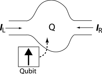
Figure 1: Schematic of the mesoscopic scattering detector, in which the current through a phase coherent scattering region is used to detect the qubit. $Q$ denotes the charge in the scattering region, while $I_{R}$ ($I_{L}$) is the current in the right (left) contact.

We start by considering the simplest situation, also considered in Ref. Pilgram, , where the state of the qubit provides a uniform potential change in the scattering region. In this case the input operator $Q$ is the total charge in the scattering region. Unlike Ref. Pilgram, , we do not explicitly consider the effects of screening here. Within an RPA scheme, consideration of such effects allows an explicit calculation of the qubit-detector coupling strength $A$, but does not result in any other changes over a non-interacting approach. In the weak coupling regime, the particular value of $A$ does not affect the approach to the quantum limit.

Letting $a_{\alpha n}^{\dagger}(E)$ represent the creation operator for an incident wave in contact $\alpha=L,R$, transverse mode $n$, and at energy $E$, the detector current operator for contact $\alpha$ takes the form ButtikerReview :

$$I_{\alpha} = \frac{e}{h}\int dE\int dE^{\prime}\sum_{\beta,\gamma=L,R}\sum_{n,m=1}^{N}$$ (27)

$$\left[a_{\beta n}^{\dagger}(E)A_{\beta n,\gamma m}(\alpha;E,E^{\prime})a_{\gamma m}^{\phantom{\dagger}}(E^{\prime})\right]$$

$$A_{\beta n,\gamma m}(\alpha;E,E^{\prime})=\delta_{\beta\gamma}\delta_{\alpha\beta}\delta_{nm}-\left(\left[s_{\alpha\beta}(E)\right]^{\dagger}s_{\alpha\gamma}(E^{\prime})\right)_{nm}$$ (28)

A positive current corresponds to a current incident on the scattering region; note that throughout this section, we neglect electron spin for simplicity. The total charge $Q$ in the scattering region may be defined in terms of the total current incident on the scattering region– in the Heisenberg picture, $\partial_{t}Q(t)=I_{L}(t)+I_{R}(t)$ . One obtains:

$$Q = e\int dE\int dE^{\prime}\sum_{\beta,\gamma=L,R}$$ (29)

$$\left[a_{\beta n}^{\dagger}(E){\mathcal{N}}_{\beta n,\gamma m}^{\phantom{\dagger}}(E,E^{\prime})a_{\gamma m}^{\phantom{\dagger}}(E^{\prime})\right]$$

$${\mathcal{N}}(E,E+\hbar\omega) = \frac{1}{2\pi i}\left[s^{{\dagger}}(E)\frac{s(E+\hbar\omega)-s(E)}{\hbar\omega}\right].$$ (30)

In the limit where $\omega\rightarrow 0$, ${\mathcal{N}}(E,E+\hbar\omega)$ reduces to the well-known Wigner-Smith delay time matrix:

$${\mathcal{N}}(E)=\frac{1}{2\pi i}\left[s^{{\dagger}}(E)\frac{d}{dE}s(E)\right]$$ (31)

Finally, the assumption that the qubit couples to the total charge in the scattering region is equivalent to assuming that the potential it creates is smooth in the WKB sense. We can use the fact that the sensitivity of the scattering matrix $s$ to a global change of potential in the scattering region is the same as its sensitivity to energy. Thus, the linear response coefficient $\lambda$ has the form:

$$\lambda = -\frac{e^{2}}{h}\int_{\mu_{R}}^{\mu_{L}}d\varepsilon\frac{d}{d\varepsilon}\left[\textrm{tr }s_{LR}^{\dagger}(\varepsilon)s_{LR}(\varepsilon)\right]$$ (32)

$$= -\frac{e^{2}}{h}\int_{\mu_{R}}^{\mu_{L}}d\varepsilon\sum_{j}\frac{dT_{j}(\varepsilon)}{d\varepsilon},$$

where the $T_{j}$ are the transmission eigenvalues of the system. Without loss of generality, we have assumed that our detector is biased such that the chemical potential of the left reservoir is greater than that of the right reservoir: $\mu_{L}-\mu_{R}=e|V|$; we also consider the limit of zero temperature.

III.1 Single Channel Case

Given these definitions, we can now turn to Eqs. (16) and (17) and ask what is required of the scattering matrix $s$ in order to reach the quantum limit. We first focus on the case $N=1$, where there is a single propagating mode in both contacts. The scattering matrix $s$ is thus $2\times 2$, and may be written as:

$$s(E)=\left(\begin{array}[]{cc}s_{LL}&s_{LR}\\ s_{RL}&s_{RR}\\ \end{array}\right)=\left(\begin{array}[]{cc}\sqrt{R}e^{i\beta}&\sqrt{T}e^{i\varphi^{\prime}}\\ \sqrt{T}e^{i\varphi}&-\sqrt{R}e^{i(\varphi+\varphi^{\prime}-\beta)}\\ \end{array}\right)$$ (33)

where $R=1-T$. At zero temperature, the detector is described by a single many-body state $|i\rangle$ in which all incident states in lead $\alpha$ with $E<\mu_{\alpha}$ are occupied, and all other incident states are unoccupied:

$$|i\rangle=\left(\Pi_{E_{L}\leq\mu_{L}}a^{{\dagger}}_{L}(E_{L})\right)\left(\Pi_{E_{R}\leq\mu_{R}}a^{{\dagger}}_{R}(E_{R})\right)|\textrm{vac}\rangle$$ (34)

First, we consider the causality condition of Eq. (17) which requires that the backwards gain $\lambda^{\prime}$ vanishes. As we know the initial state of the detector and have explicit expressions for $I$ and $Q$, we can directly evaluate the function $S_{IQ}(E)$ appearing in Eq. (18) in terms of $s$. A direct calculation can be performed to show that:

$$\int_{-\infty}^{\infty}dE\frac{\textrm{Re }\left[S_{IQ}(E)\right]}{E} = \int_{-\infty}^{\infty}dE\frac{\textrm{Re }\left[F(E)\right]}{E}$$ (35)

$$\textrm{Im }\left[S_{IQ}(0)\right] = \textrm{Im }\left[F(0)\right]$$ (36)

where, letting $t\equiv s_{RL}$,the function $F(E)$ is defined as:

$$F(E)=-i\frac{e^{2}}{2\pi}\int_{\mu_{R}}^{\mu_{L}}dE^{\prime}t^{*}(E^{\prime})\left(\frac{t(E^{\prime}+E)-t(E^{\prime})}{E}\right)$$ (37)

Note that Eqs. (35) and (36) are independent of whether $I$ is take to be $I_{L}$, $I_{R}$, or a linear combination of the two. Now, causality dictates that the scattering matrix $s$ is analytic in the upper half complex plane, and thus so is the function $F(E)$. The real and imaginary parts of $F$ are thus related by a Hilbert transform, and Eqs. (20), (35) and (36) imply that $\lambda^{\prime}=0$ for the scattering detector irrespective of the choice of s. Thus, the causality properties of the scattering matrix $s$ ensure that one of the conditions necessary for reaching the quantum limit is always satisfied. Note that substituting these expressions for $S_{IQ}(E)$ in Eq. (19) does indeed yield the expected form of $\lambda$ (Eq. (32)). It is also useful to note that gauge invariance can be used to directly establishLevitov $\lambda^{\prime}=0$ . The essence of the argument is that a coupling to the current (i.e. $H_{\rm int}=A\sigma_{z}I(x=0)$) is equivalent to introducing a local vector potential. The gauge transformation which removes this term will only modify the transmission phases in the scattering matrix $s$ (i.e. $\phi$ and $\phi^{\prime}$) in an energy-independent manner. Using Eq. (29), one can check that $\langle Q\rangle$ is independent of energy-independent phase changes; thus $\lambda^{\prime}=0$.

Next, we turn to the condition given in Eq. (16), which requires a certain proportionality between $\widetilde{I}$ and $\widetilde{Q}$ in order to reach the quantum limit. Given the state $|i\rangle$ which describes the detector (Eq. (34)), the only matrix elements of $I$ and $Q$ which contribute to the zero frequency noise correlators (c.f. Eqs (4)) involve energy-conserving transitions where a scattering state incident from the left reservoir is destroyed while a scattering state incident from the right reservoir is created. Since these transitions require an occupied initial state and an unoccupied final state, they can only occur in the energy interval $\mu_{R}<E<\mu_{L}$. We are thus interested in the coefficients of the operators $a_{R}^{\dagger}(E)a_{L}^{\phantom{\dagger}}(E)$ appearing in the expansion of $I$ and $Q$ in this energy interval. The proportionality requirement of Eq. (16) thus results in a necessary condition on $s(\varepsilon)$:

$$\forall E\epsilon[\mu_{R},\mu_{L}],\hskip 5.69046pt\left[s_{LR}\right]^{*}(E)s_{LL}^{\phantom{*}}(E)=i{\mathcal{C}}{\mathcal{N}}_{RL}(E)$$ (38)

where ${\mathcal{C}}$ is a real, energy-independent constant. Using Eq. (33), the imaginary and real parts of the above condition become:

$$\forall E\epsilon[\mu_{R},\mu_{L}],\hskip 5.69046pt\frac{d}{dE}\left(\beta(E)-\phi(E)\right) = 0$$ (39)

$$\frac{\frac{dT}{dE}(E)}{T(E)(1-T(E))} = -\frac{4\pi}{{\mathcal{C}}}$$ (40)

Similar conditions for reaching the quantum limit for this version of the scattering detector were first developed in Ref. Pilgram, by directly calculating $\Gamma_{\rm meas}$ and $\Gamma_{\varphi}$ (note there is a sign error in Eq. (7) of Ref. Pilgram, which must be corrected to obtain our Eq. (39)). ConstantNote The fulfilling of these conditions does not correspond to symmetries usually considered in mesoscopic systems; for example, as we will show, the presence of time-reversal symmetry is not a necessary requirement. Instead, the conditions of Eqs. (39) and (40) correspond directly to the requirement that there be no missing information in the detector, information which is not revealed in a measurement of $\langle I\rangle$. We demonstrate this explicitly in what follows.

III.1.1 Phase Condition

The first condition (Eq. (39)) for reaching the quantum limit requires that the difference between transmission and reflection phases in the scattering matrix be constant in the energy interval defined by the voltage. If it holds, changing the state of the qubit will not modulate this phase difference. Eq. (39) thus constrains information– it ensures that the detector does not extract additional information about the qubit which resides in the relative phase between transmission and reflection. Such information is clearly not revealed in a measurement of $\langle I\rangle$, and would necessarily lead to additional dephasing over and above the measurement rate. In principle, this additional information could be extracted by performing an interference experiment. To be more specific, note that the cross-correlator $S_{IQ}$ (c.f. Eq. 4c) is given by:

$$S_{IQ}=i\hbar\lambda+\frac{e^{2}}{\pi}\int_{\mu_{R}}^{\mu_{L}}dE^{\prime}\left(T(1-T)\frac{d}{dE}(\beta-\varphi)\right)$$ (41)

By definition, the imaginary part of this correlator determines the linear response coefficient $\lambda$ (c.f. Eq. (3)) associated with measuring $\langle I\rangle$. In contrast, the real part of this correlator may be interpreted as the linear response coefficient associated with a measurement where one interferes reflected and transmitted electrons; the factor of $T(1-T)$ corresponds to the fact that the magnitude of this signal will be proportional to the amplitude of both the reflected and transmitted beams. More explicitly, consider the Hermitian operator $I_{\rm mod}$ defined by:

$$I_{\rm mod}=\frac{e}{\hbar}\int_{\mu_{R}}^{\mu_{L}}dE\left[ia_{R}^{\dagger}(E)A_{RL}(L;E,E)a_{L}^{\phantom{\dagger}}(E)+h.c.\right]$$ (42)

If one were to now measure $I_{\rm mod}$, the corresponding linear response coefficient $\lambda_{\rm mod}$ is precisely the real part of $S_{IQ}$ (this can be seen by comparing Eqs. (42) and (27) ). The fact that additional information on the state of the qubit is available in the expectation $\langle I_{\rm mod}\rangle$ implies that the qubit is entangling with the detector faster than the measurement rate associated with $\langle I\rangle$. This remains true even if one does not explicitly extract this information, as was demonstrated recently in the experiment of Sprinzak et. al. Heiblum

Stepping back, we see that the general condition $\textrm{Re }S_{IQ}=0$ (i.e. the required factor of $i$ on the RHS of Eq. 16) needed to reach the quantum limit directly corresponds to the requirement of no “missing” information discussed in the previous subsection. In general, a non-vanishing $\textrm{Re }S_{IQ}$ implies that additional information about the qubit’s state could be obtained by simultaneously measuring another quantity in addition to $I$ (e.g., in our case, the quantity $I_{\rm mod}$).

Note that in the scattering detector, the symmetry required to ensure that Eq. (39) holds (i.e. that the phases $\beta$ and $\phi$ coincide) is not one that is usually considered in mesoscopic systems. In particular, the presence of time-reversal symmetry is not necessary to fulfilling the condition of Eq. (39); time-reversal symmetry only implies that $\varphi=\varphi^{\prime}$, and specifies nothing on the relation between $\varphi$ and $\beta$. However, as pointed out in Ref. Pilgram, , a sufficient condition for achieving Eq. (39) is that one has parity symmetry, that is both time-reversal symmetry and left-right inversion symmetry (the latter condition implies that the two reflection phases in $s$ are identical).SymmNote Note that this is not a necessary condition. We see that the required symmetry here is best understood as being related to information.

III.1.2 Transmission Condition

We now turn to the second condition (Eq. (40)) needed to have the scattering detector reach the quantum limit, a condition which constrains the energy dependence of the transmission probability $T$. This condition arises from the requirement that the proportionality between $I$ and $Q$ needed for the quantum limit must hold over the entire energy interval defined by the voltage. In general, energy averaging causes a departure from the quantum limit– over sufficiently large intervals, the operators $I$ and $Q$ look less and less like one another. Like Eq. (39), Eq. (40) can also be interpreted as a requirement of no “missing” information. Here, the requirement is that energy averaging does not result in the loss of information about the qubit which is encoded in the energy dependence of $T$. While such information is not obtained in a measurement of $\langle I\rangle$ (which involves energy averaging, c.f. Eq. (32)), it could be obtained if one measured the entire function $\langle I(V)\rangle$ for $0\leq|V|\leq\mu_{L}-\mu_{R}$. As discussed, the presence of any missing information necessarily implies a departure from the quantum limit.

Interestingly enough, Eq. (40) may be understood completely classically, even though it formally results from requiring the proportionality of two quantum operators. To do so, we calculate the classical information capacity $R$ (c.f. Eq. (21)) corresponding to two different possible measurements. First, imagine we measure the integrated current $m=\int_{0}^{t}dt^{\prime}I(t^{\prime})$, and assume the probability distributions $p(m|\uparrow)$ and $p(m|\downarrow)$ are Gaussian. For weak coupling, one finds for the capacity:

$$R_{\rm avg}=\Gamma_{\rm meas}t = \frac{t}{2h}\frac{\left(eA\int_{\mu_{R}}^{\mu_{L}}d\varepsilon\frac{dT(\varepsilon)}{d\varepsilon}\right)^{2}}{\int_{\mu_{R}}^{\mu_{L}}d\varepsilon T(\varepsilon)(1-T(\varepsilon))}$$ (43)

$$\simeq \frac{(\delta\varepsilon)t}{2h}\frac{\left(eA\sum_{j}\frac{dT(\varepsilon_{j})}{d\varepsilon}\right)^{2}}{\sum_{j}T(\varepsilon_{j})(1-T(\varepsilon_{j}))}$$ (44)

In the last line, we have discretized the energy integrals i.e. partitioned the interval $[\mu_{R},\mu_{L}]$ into equal segments of length $\delta\varepsilon$. If we now imagine we could measure each $m_{j}=\int_{0}^{t}I_{j}(t)$, where $I_{j}(t)$ is the contribution to the current from the $j$th energy interval, a similar calculation reveals:

$$R_{\rm tot} = \frac{(\delta\varepsilon)t}{2h}\sum_{j}\frac{\left(eA\frac{dT(\varepsilon_{j})}{d\varepsilon}\right)^{2}}{T(\varepsilon_{j})(1-T(\varepsilon_{j}))}$$ (45)

One can easily check that $R_{\rm tot}\geq R_{\rm avg}$; this corresponds to the additional information that is generally available in the energy dependence of $T$. A necessary and sufficient condition for ensuring $R_{\rm tot}=R_{\rm avg}$ is precisely the condition of Eq. (40). On a purely classical level, this condition ensures that no information is lost when one averages over energy.

How can the problems generally posed by energy averaging be avoided? One possible solution would be to use voltages small enough that the scattering matrix $s$ can be approximated as being linear in energy, that is $eV(dT/dE)\ll 1$ (this is the approach of Ref. Pilgram, ). However, as the linear response coefficient $\lambda$ is given by the energy derivative of the transmission (c.f. Eq. (32)), such a small voltage would imply both a small signal and essentially no gain. The change in current induced by the qubit, $\Delta I=\pm A\lambda$, would be much smaller than the current associated with the coupling voltage $A$:

$$\lambda \simeq \frac{e^{2}}{h}\left(\frac{dT}{dE}e|V|\right)\ll\frac{e^{2}}{h}$$ (46)

$$\Gamma_{\rm meas} \propto \left(\frac{dT}{dE}eV\right)^{2}\left(\frac{A}{eV}\right)\frac{A}{h}\ll\frac{A}{h}$$ (47)

Even though this smallness of $\lambda$ does not theoretically affect the approach to the quantum limit, it does severely limit the detector’s practical value– for very slow measurement rates, environmental effects on the qubit will become dominant over backaction effects.

If we now consider finite voltages and fully energy-dependent scattering, Eq. (40) tells us the condition under which energy averaging the transmission does not impede reaching the quantum limit. The solution to Eq. (40) has the form:

$$T(E)=\frac{1}{1+e^{4\pi(E-E_{0})/{\mathcal{C}}}}$$ (48)

This form for $T(E)$ implies that there is no extra information in the energy dependence of $T$ which is lost upon energy averaging. Amusingly, Eq. (40) corresponds exactly to the energy-dependent transmission of one channel of an adiabatic quantum point contact GlazmanQPC . The constant $E_{0}$ represents the threshold energy of the channel (i.e. the transverse mode), and the constant ${\mathcal{C}}$ is given by:

$${\mathcal{C}}=-\frac{2\sqrt{2}\hbar v_{F}}{\sqrt{dR}}$$ (49)

where $d$ is the transverse width of the constriction at its center, and $R$ is the radius of curvature of the transverse confining potential at the constriction center.

III.2 Multichannel Case

We now consider the situation where there are $N$ channels in each of the two contacts leading to the reservoirs. It is useful to write $s$ in terms of its $N$ transmission eigenvalues $T_{j}(E)$ using the standard polar decomposition:BeenakkerRMT

$$s(E)=\left(\begin{array}[]{cc}s_{LL}&s_{LR}\\ s_{RL}&s_{RR}\end{array}\right)=\left(\begin{array}[]{c}U\\ V\end{array}\right)\left(\begin{array}[]{cc}\sqrt{R}&\sqrt{T}\\ \sqrt{T}&-\sqrt{R}\end{array}\right)\left(\begin{array}[]{c}U^{\prime}\\ V^{\prime}\end{array}\right)$$ (50)

Here, $U,U^{\prime},V,V^{\prime}$ are $N\times N$ energy-dependent unitary matrices, and $\sqrt{R}$ and $\sqrt{T}$ are diagonal matrices having entries $\sqrt{1-T_{j}(E)}$ and $\sqrt{T_{j}(E)}$, respectively.

In the multichannel case, the backwards gain $\lambda^{\prime}$ again vanishes irrespective of the details of $s$ as a result of the analytic properties of $s$. The relevant question then to ask is what conditions must be satisfied by $s(E)$ so that the proportionality between $I$ and $Q$ required to reach the quantum limit (i.e. Eq. (16) ) is achieved. As in the single-channel case, the relevant matrix elements of $I$ and $Q$ involve destroying a scattering state incident from the left and creating an equal-energy state describing an incident wave from the right; the additional complication now is that these transitions could result in a change of transverse mode. One thus needs to examine the coefficients of the operator products $a_{Rn}^{\dagger}(E)a_{Lm}^{\phantom{\dagger}}(E)$ appearing in the expansion of $I$ and $Q$, in the energy interval $[\mu_{R},\mu_{L}]$. The proportionality condition of Eq. (16) again yields the requirement that Eq. (38) hold for all energies in this interval; now, however, both the right and left-hand side of this equation are $N\times N$ matrices:

$$\forall E\epsilon[\mu_{R},\mu_{L}],\hskip 5.69046pt\left[s_{LR}(E)\right]^{\dagger}s_{LL}^{\phantom{\dagger}}(E)=i{\mathcal{C}}{\mathcal{N}}_{RL}(E)$$ (51)

Here, ${\mathcal{C}}$ is again an energy-independent real number. Using the polar decomposition, one can derive from Eq. (51) two necessary matrix conditions which must hold for all energies in the interval defined by the voltage:

$$\sqrt{T(E)}\phi_{U}(E)\sqrt{R(E)}-\sqrt{R(E)}\phi_{V}(E)\sqrt{T(E)}=0$$ (52)

$$\frac{\frac{dT}{dE}(E)}{T(E)(1-T(E))}=-\frac{4\pi}{{\mathcal{C}}}\times\hat{1}$$ (53)

These conditions are the multi-channel analogs of Eqs. (39) and (40). $\hat{1}$ denotes the $N\times N$ unit matrix, and we have introduced the generalized “phase-derivative” Hermitian matrices $\phi_{U}$ and $\phi_{V}$:

$$\phi_{U}(\varepsilon) = -iU^{{\dagger}}(\varepsilon)\left[\frac{d}{dE}U(\varepsilon)\right]$$ (54)

$$\phi_{V}(\varepsilon) = -iV^{{\dagger}}(\varepsilon)\left[\frac{d}{dE}V(\varepsilon)\right]$$ (55)

These matrices play the role of the energy-derivatives of the phases $\beta$ and $\phi$ in the single channel case. Note the evident asymmetry in Eq. (52): the polar decomposition matrices $U$ and $V$ enter, but the matrices $U^{\prime}$ and $V^{\prime}$ do not. We comment on this in what follows.

III.2.1 Phase and Channel Mixing Conditions

The first requirement (Eq. (52)) places a stringent requirement on the scattering matrix $s$. Like the corresponding requirement for the single-channel system, it ensures that there is no additional information on the state of the qubit available in measurable changes of scattering phases. Again, time-reversal symmetry is not necessary to have this condition hold, as time-reversal symmetry only ensures $U=U^{\prime}$ and $V=V^{\prime}$. However, unlike the single-channel case, even the presence of parity symmetry (i.e. the combination of both time-reversal symmetry and left-right inversion symmetry) is not sufficient to guarantee that Eq. (52) is satisfied. The presence of parity symmetry would indeed ensure $\phi_{U}=\phi_{V}$, but as in general $\left[\sqrt{T},\phi_{U}\right],\left[\sqrt{R},\phi_{U}\right]\neq 0$, this is not enough. In addition to having $\phi_{U}=\phi_{V}$, one also generally needs either that $\phi_{U}$ is diagonal, meaning that the mode index (i.e. transverse momentum) is conserved during scattering, or that all the transmission eigenvalues $T_{j}$ are identical. We thus see that if the transmissions fluctuate, mode-mixing (e.g. the non-conservation of transverse energy) also prevents one from reaching the quantum limit of detection. This can be understood from the point of view of information. If the $\phi_{U},\phi_{V}$ matrices are not purely diagonal, information about the qubit could be gained by looking at changes in how electrons incident in a given mode are partitioned into outgoing modes. Such changes would not be detectable if all channels had the same transmission. Note that the matrices $U^{\prime}$ and $V^{\prime}$ appearing in the polar decomposition of $s$ (Eq. (50)) are irrelevant to reaching the quantum limit. As each transverse mode is equally populated with incoming waves in the state $|i\rangle$, there is no information associated with the preferred mode structure for incoming waves (i.e. the eigenvectors of $U^{\prime}$ and $V^{\prime}$).

III.2.2 Transmission Condition

Consider now the condition imposed by Eq. (53), which constrains the form of the transmissions $T_{j}(\varepsilon)$ of the detector. Similar to the corresponding condition for the single-channel system, this requirement ensures that there is no additional information available in either the energy or channel structure of the $\{T_{j}(\varepsilon)\}$ which is lost upon averaging. One obtains a necessary form for the transmissions, similar to what was found in Ref. Pilgram, :

$$T_{j}(E)=\frac{1}{1+e^{4\pi(E-E_{j})/{\mathcal{C}}}}$$ (56)

Note that different modes differ from one another only by their threshold energy $E_{j}$; the constant ${\mathcal{C}}$ is the same for each mode. Again, this form for the transmissions {$T_{j}(\varepsilon)$} corresponds exactly to those expected for a multi-channel adiabatic point contact.GlazmanQPC The assumption of adiabaticity implies that transverse energy is conserved. Thus, if parity symmetry also holds, we reach the surprising conclusion that a multi-channel adiabatic point contact remains a quantum limited detector even if the voltage is large enough that several modes contribute to transport. Previous studies have established that point contact detectors reach the quantum limit in the limit of small voltages, where the energy-dependence of scattering can be neglected Gurvitz ; Stodolsky ; KorotkovQPC . We have shown here that in the adiabatic case, the quantum limit continues to hold even at voltages large enough that the energy dependence of scattering is important. This is significant from a practical standpoint– requiring small voltages limits the magnitude of the output current and thus the overall scale of the measurement rate, making the detector more susceptible to environmental effects.

III.2.3 General Expression for Noise Correlators

For completeness, we give explicit expressions for the noise correlators. Writing them in terms of energy dependent $N\times N$ matrix kernels (i.e. $S_{X}=\int_{\mu_{R}}^{\mu_{L}}d\varepsilon\left[\textrm{tr }\hat{S}_{X}(\varepsilon)\right]$) we obtain:

$$\hat{S}_{I}(\varepsilon) = \frac{2e^{2}}{h}T(1-T)$$ (57a)

$$\hat{S}_{Q}(\varepsilon) = \frac{e^{2}\hbar}{2\pi}\Bigg{(}\frac{\left(\partial_{\varepsilon}T\right)^{2}}{2T(1-T)}+2TR\left(\phi_{U}-\phi_{V}\right)^{2}$$ (57b)

$$+2\left[\phi_{U},\sqrt{TR}\right]\left[\sqrt{TR},\phi_{V}\right]$$

$$+\left[\phi_{U},T\right]\left[T,\phi_{U}\right]+\left[\phi_{V},T\right]\left[T,\phi_{V}\right]\Bigg{)}$$

$$\hat{\lambda}(\varepsilon) = -\frac{e^{2}}{h}\left(\partial_{\varepsilon}T\right)$$ (57c)

$$\hat{S}_{IQ}(\varepsilon) = i\hbar\hat{\lambda}(\varepsilon)+\frac{e^{2}}{\pi}\left[\sqrt{TR}\left(\phi_{U}-\phi_{V}\right)\right]$$ (57d)

A similar expression for the charge noise $S_{Q}$ of a mesoscopic conductor was first derived by Büttiker EarlyButtiker . Unlike the expression for the current noise $S_{I}$, which can easily be understood in terms of partition noise, it would seem at first that there is no simple, heuristic way to interpret the expression for $S_{Q}$. However, if we invoke ideas of information, each term in Eq. (57b) acquires a simple meaning. The first term represents information associated with the energy dependence of the transmissions; the second, information associated with the energy dependence of phase differences; and the last three terms, information associated with the partitioning of electrons into different modes. In general, using Eqs. (5) and (25), we may define the charge noise in terms of the accessible information ${\mathcal{I}}$ in the coupled conductor plus qubit system:

$$S_{Q}=\lim_{A\rightarrow 0}\lim_{t\rightarrow 0}\frac{\hbar^{2}}{A^{2}}\frac{d}{dt}{\mathcal{I}}(t)$$ (58)

While this last expression may seem purely tautological, it is clear that the various contributions to Eq. (57b) for the charge noise are best understood in terms of information. Note that the accessible information ${\mathcal{I}}$ could be obtained directly in the present system by calculating the overlap between the detector states corresponding to the two qubit states. Such a calculation would take the form of an orthogonality catastrophe calculation, similar to that presented in Ref. Aleiner, .

III.3 Local Potential Coupling

In the remaining part of this paper, we consider a more general version of the mesoscopic scattering detector, showing that the main results of the previous section continue to hold. We relax the condition that the state of the qubit modulates a uniform potential in the scattering region, thus allowing for a wider class of input operators $Q$ than that given in Eq. (29). In general, we may write:

$$Q = e\int dEdE^{\prime}\sum_{\beta,\gamma=L,R}$$

$$\left[a_{\beta n}^{\dagger}(E)W_{\beta n,\gamma m}^{\phantom{\dagger}}(E,E^{\prime})a_{\gamma m}^{\phantom{\dagger}}(E^{\prime})\right]$$

where $W(E,E^{\prime})$ is a $2N\times 2N$ Hermitian matrix having dimensions of inverse energy. The situation considered in the last section corresponds to choosing $W$ to be ${\mathcal{N}}(E,E^{\prime})$ (Eq. (30)), which at $E=E^{\prime}$ is just the Wigner-Smith delay time matrix. By comparing against the current operator $I$ (c.f. Eq. (27)), it is clear that the proportionality condition of Eq. (16) necessary for the quantum limit constrains the diagonal in energy, off-diagonal in lead index part of the potential matrix $W$:

$$\forall E\epsilon[\mu_{R},\mu_{L}],\hskip 5.69046pt\left[W(E,E)\right]_{RL}=i\frac{1}{{\mathcal{C}}}\left[s_{LR}\right]^{\dagger}(E)s_{LL}^{\phantom{\dagger}}(E)$$ (60)

where ${\mathcal{C}}$ is a real constant . We thus see that the required proportionality between $I$ and $Q$ needed to reach the quantum limit at zero temperature leaves a large part of the potential matrix $W$ undetermined (i.e. terms diagonal in the lead index and/or off-diagonal in energy). We now show that by considering a form for $W$ which is drastically different from ${\mathcal{N}}$, one can make it easier to reach the quantum limit and have a reasonable gain. In particular, one can work at small voltages without necessarily having a vanishing gain.

We specialize the discussion to a case which in many ways is the opposite of having global potential coupling. We take the scattering matrix $s$ to be energy-independent over the energy interval defined by the voltage, and take $W$ to correspond to a local potential: $W(E,E^{\prime})=W$ over the energies of interest. In this case, the scattering matrix $s$ will have one of two different energy-independent values depending on the state of the qubit:

$$s_{\pm}=s_{0}\pm eA\left(\Delta s\right)$$ (61)

where $s_{0}$ is the scattering matrix at zero coupling ($A=0$). The matrix $W$ may be directly related to the change in the scattering matrix, $\Delta s$ (see Appendix B for a derivation):

$$W=is_{0}^{\dagger}\left(\Delta s\right)$$ (62)

Note the similarity to the form of $W$ in the global-potential coupling case (where $W={\mathcal{N}}$); now, the energy derivative $ds/dE$ has been replaced by the finite difference $\Delta s\equiv(s_{+}-s_{-})/(2eA)$.

Turning to the conditions needed for the quantum limit, we find again that the causality properties of the scattering matrices $s_{\pm}$ ensure $\lambda^{\prime}=0$ always. The remaining proportionality requirement of Eq. (16) places constraints on $s_{\pm}$. These have an analogous form to Eqs. (53) and (52), but now the energy derivative $d/dE$ is replaced by the finite difference $\Delta$ (i.e. $\Delta X=(X[s_{+}]-X[s_{-}])/(2eA)$):

$$\frac{\Delta T}{T(1-T)}={\mathcal{C}}\times\hat{1}$$ (63)

$$\sqrt{T}\widetilde{\phi}_{U}\sqrt{R}-\sqrt{R}\widetilde{\phi}_{V}\sqrt{T}=0$$ (64)

where $\widetilde{\phi}_{U}=-iU^{\dagger}(\Delta U)$, $\widetilde{\phi}_{V}=-iV^{\dagger}(\Delta V)$ . Importantly, the above conditions do not involve any energy averaging, as we have taken $s$ and $W$ to be energy independent. Nonetheless, there still is a non-vanishing gain $\lambda$ determined by both the voltage and the $\Delta T_{j}$:

$$\lambda=\frac{e^{2}V}{h}\sum_{j}\Delta T_{j}$$ (65)

Thus, using a local coupling between the qubit and the scattering detector makes it easier to reach the quantum limit and have a sizeable gain– one can use voltages small enough that energy-averaging is not a problem, while still having the qubit modulate the transmissions. Note that in the single channel case, all that is needed for the quantum limit is that the state of the qubit not change the difference between reflected and transmitted phases: $\Delta(\phi-\beta)=0$. Also note the various noise correlators are given by Eqs. (57), with the substitution $d/dE\rightarrow\Delta$.

IV Conclusions

We have developed a general set of conditions which are needed for a detector in the linear-response regime to reach the quantum limit of detection. One needs both a restricted proportionality between the input and output operators of the detector (c.f. Eq. (16)), and a causal relation between the output and input (c.f. Eq. (17)). Applying the concept of accessible information to the detector, one sees that deviations from the quantum limit imply the existence of “missing” information residing in the detector, information which is not being utilized. The general conditions of Eqs. (16) and (17) ensure the non-existence of such information. Applying these concepts to the mesoscopic scattering detector, we find that these general conditions place restrictions on the form of the detector’s scattering matrix. These restrictions do not involve symmetry properties usually considered in mesoscopic systems, but are rather best understood as following from the requirement of having no missing information. In the mesoscopic scattering detector, missing information may reside in the relative phase between transmission and reflection, in the energy or mode structure of the transmission probabilities, or in the partitioning of scattered electrons between different modes. Surprisingly, we find that an adiabatic point contact conforms to all the conditions needed for the quantum limit, even when the voltage is large enough that many modes are involved in transport, and the energy dependence of scattering is important.

We thank M. Devoret for useful conversations. This work was partially supported by ARDA through the Army Research Office, grant number DAAD19-02-1-0045, by the NSF under Grants No. DMR-0084501 and DMR-0196503, and by the W. M. Keck Foundation.

Appendix A Accessible Information

In this appendix, we provide a simple proof of Eq. (24) for the accessible information $\mathcal{I}$. Given the two states $|D_{\uparrow}\rangle$ and $|D_{\downarrow}\rangle$, the goal is to maximize the classical mutual information $R$ (defined in Eq. (21)) over all possible choices of measurements. A given choice of measurement $Y$ corresponds to a choice of basis; the probability distributions $p(y_{i}|\uparrow)$ and $p(y_{i}|\downarrow)$ are determined by the elements of the corresponding states in this basis. Treating the $p(y_{i}|\sigma)$ as independent variables restricted to the interval $[0,1]$, and using Lagrange multipliers, we minimize $R$ subject to the following constraints:

$$\sum_{i=1}^{N}p(y_{i}|\sigma) = 1$$ (66)

$$\sum_{i=1}^{N}\sqrt{p(y_{i}|\uparrow)p(y_{i}|\downarrow)} = |\langle D_{\uparrow}|D_{\downarrow}\rangle|\equiv\cos\alpha$$ (67)

The second condition in principle need only be an inequality, with the left-hand side being greater than or equal to the right-hand side; however, it can be verified that the maximum value of $R$ occurs when it is enforced as an equality. Also note that without loss of generality, we can choose the inner product appearing in Eq. (67) to be real and positive, as $R$ is independent of the relative phase between the states $|D_{\sigma}\rangle$. Finally, we have assumed to start that these states have at most $N$ non-zero components in the chosen basis. Variation with respect to $p(y_{i}|\uparrow)$ yields the condition:

$$\log\frac{p(y_{i}|\uparrow)}{\bar{p}(y_{i})}+2\lambda_{\uparrow}+\lambda\sqrt{\frac{p(y_{i}|\downarrow)}{p(y_{i}|\uparrow)}}=0,$$ (68)

with a similar equation emerging from variation with respect to $p(y_{i}|\downarrow)$. $\lambda$, $\lambda_{\uparrow}$ and $\lambda_{\downarrow}$, are Lagrange multipliers; $\bar{p}(y_{i})=\left[p(y_{i}|\uparrow)+p(y_{i}|\downarrow)\right]/2$ is the averaged distribution. Subtracting the $\uparrow$ and $\downarrow$ equations yields:

$$\lambda = \frac{\sqrt{p(y_{i}|\downarrow)p(y_{i}|\uparrow)}}{p(y_{i}|\uparrow)-p(y_{i}|\downarrow)}\log\frac{p(y_{i}|\uparrow)}{p(y_{i}|\downarrow)}$$ (69)

$$= \frac{\sqrt{1-\beta_{i}^{2}}}{2\beta_{i}}\log\frac{1+\beta_{i}}{1-\beta_{i}}$$

where we have defined $\beta_{i}$ via

$$\beta_{i}=\frac{p(y_{i}|\uparrow)-p(y_{i}|\downarrow)}{\bar{p}(y_{i})}$$ (70)

$\beta_{i}$ may be thought of as the amount of information gained in a measurement given that the outcome of the measurement is $y_{i}$. Now, Eq. (69) must hold for each $\beta_{i}$ ($i=1...N$); moreover, the function on the right-hand side is symmetric in $\beta_{i}$ and monotone decreasing for $0\leq\beta_{i}\leq 1$. It thus follows that for each $i$,

$$(\beta_{i})^{2}=\textrm{constant}=\sin^{2}\alpha$$ (71)

The last equality follows from substitution into Eq. (67). Further substitution into Eq. (21) for $R$ yields the expression in Eq. (24); note that the averaged distribution $\bar{p}(y_{i})$ and the relevant number of basis elements $N$ do not appear in this expression. One can explicitly check that choosing any of the $p(y_{i}|\sigma)$ to be $0$ or $1$ results in a lower value of $R$; thus, Eq. (24) does indeed correspond to the maximum value of $R$ and thus, by definition, to the accessible information $\mathcal{I}$. The condition Eq. (71) required to optimize $R$ implies that the amount of information gained via measurement is the same for each of the measurement outcomes $y_{i}$. Equivalently, each basis element in an optimal basis has the same information content associated with it. This is similar to requirements obtained to have the mesoscopic scattering detector reach the quantum limit; in that case, each channel and each energy were required to have the same information content (c.f. Eq. (53)). Note also that there are several distinct choices of bases (i.e. measurement schemes) which optimize $R$; this point was not made in Ref. Levitin, . A particularly simple optimal basis can be constructed for $N=2$. In this basis, the non-zero components of the states $|D_{\sigma}\rangle$ are given by:

$$|D_{\uparrow}\rangle=(\cos\theta,\sin\theta)\hskip 28.45274pt|D_{\uparrow}\rangle=(\sin\theta,\cos\theta)$$ (72)

where $\theta=\pi/4+\alpha/2$. By definition, the state $(1,0)$ leads to the measurement outcome $y_{1}$ with perfect certainty, while the state $(0,1)$ leads to the measurement outcome $y_{2}$ with perfect certainty. In geometric terms, the optimal basis given here is one in which the angle between the two states $|D_{\sigma}\rangle$ is bisected by the vector $(1,1)$.

More generally, consider the form of an optimal basis where $N=M$ (i.e. there are $M$ possible outcomes when a measurement is made on the state $|D_{\uparrow}\rangle$ or $|D_{\downarrow}\rangle$). Taking $M$ to be even for simplicity, and letting $|j\rangle$ denote the basis states, a possible optimal basis is one in which:

$$\langle j|D_{\uparrow}\rangle = \sqrt{\frac{1+(-1)^{j}\sin\alpha}{M}}$$ (73)

$$\langle j|D_{\uparrow}\rangle = \sqrt{\frac{1-(-1)^{j}\sin\alpha}{M}}$$ (74)

The fact that there are many possible outcomes of a measurement does not degrade from the optimality of mutual information $R$, as the information associated with each measurement outcome is the same.

Appendix B Derivation of $\Delta s$

In this Appendix, we provide a brief derivation of Eq. (62) which relates the coupling potential matrix $W$ (c.f. Eq. (III.3) ) to the associated change in the scattering matrix, $\Delta s$. The latter quantity determines the noise correlators and gain of the local-potential coupling version of the mesoscopic scattering detector. Our approach is similar to that used in Ref. AGB, to relate the scattering matrix of a quantum dot to its Hamiltonian.

In what follows, we assume (as in Sec. II B) that the potential matrix $W$ and the zero-coupling scattering matrix $s$ are independent of energy on the scales of interest. We start by writing the system Hamiltonian in terms of the scattering states of problem at zero coupling, assuming the qubit is frozen in the $\uparrow$ state:

$$H = \hbar v_{F}\sum_{m}\int dk\Bigg{[}k\,\ \psi^{{\dagger}}_{m}(k)\psi^{\phantom{\dagger}}_{m}(k)+$$ (75)

$$(Ae)\sum_{m^{\prime}}\int dk^{\prime}\left(\psi^{{\dagger}}_{m^{\prime}}(k^{\prime})W_{m^{\prime}m}\psi^{\phantom{\dagger}}_{m}(k)\right)\Bigg{]}$$

We have assumed a linear dispersion near the Fermi energy, with $\hbar k$ and $\hbar k^{\prime}$ representing the deviation of the momentum from the Fermi momentum. We have also neglected the fact that the effective Fermi velocity is channel dependent ($v_{F}$ drops out of all final expressions). The operator $\psi^{\dagger}_{m}(k)$ creates a scattering state incident in the lead and transverse mode indexed by $m$. For definiteness, we take our leads (both left and right) to be defined only on the half-line $x<0$, and to be confined in the $y$ and $z$ directions. Further, we assume that the scattering region is situated on $x>0$. We may write the full electron field operator in terms of the $\psi_{m}(k)$ operators, using the zero-coupling scattering matrix $s$. Writing $\vec{x}=(x,y,z)$, we have:

$$\Psi(\vec{x}) = \sum_{m}\int\frac{dk}{\sqrt{4\pi}}\psi_{m}(k)\Bigg{[}e^{i(k_{F}+k)x}\phi_{m}(y,z)+$$ (77)

$$\sum_{n}e^{-i(k_{F}+k)x}\phi_{n}(y,z)s_{nm}\Bigg{]}$$

$$= \frac{1}{\sqrt{2}}\sum_{m}\psi_{m}(-x)e^{ik_{F}x}\phi_{m}(y,z)+$$

$$\frac{1}{\sqrt{2}}\sum_{m,n}\psi_{m}(x)e^{-ik_{F}x}\phi_{n}(y,z)s_{nm}$$

In the last line, we have introduced the operators $\psi_{m}(x)$, which are the Fourier transforms of the scattering state operators $\psi_{m}(k)$. Note again that this expression is only valid for $x<0$, as the leads are only defined on $x<0$. We thus see that for $x<0$, $\psi_{m}(x)$ describes an outgoing (i.e. left-moving) wave, while $\psi_{m}(-x)$ describes an incoming (i.e. right-moving) wave.

Next, we may express the system Hamiltonian in terms of the $\psi_{m}(x)$ operators. This in turn leads to an equivalent single-particle Schrödinger equation:

$$E\widetilde{\psi}_{m}(E,x)= \hbar v_{F}\Big{[}i\partial_{x}\widetilde{\psi}_{m}(E,x)+$$ (78)

$$Ae\delta(x)\sum_{n}W_{mn}\widetilde{\psi}_{n}(E,x)\Big{]}$$

Here, $\widetilde{\psi}_{m}(E,x)$ is a wavefunction which arises when the field operator $\psi_{m}(x)$ is expressed in terms of operators corresponding to the eigenmodes of the full Hamiltonian $H$. Given the relation of $\psi_{m}(x)$ to incoming and outgoing waves (c.f. Eq. (77)), we choose the following form for $\widetilde{\psi}_{m}(x)$:

$$\widetilde{\psi}_{m}(E,x)=\begin{cases}e^{-ikx}a_{\textrm{in},m}&\text{if $x>0$},\\ e^{-ikx}\sum_{n}s^{{\dagger}}_{mn}a_{\textrm{out},n}&\text{if $x<0$},\end{cases}$$ (79)

where $E=\hbar v_{F}k$. Substituting this form into Eq. (77), we see that the coefficients $a_{\textrm{in},m}$ and $a_{\textrm{out},m}$ do indeed correspond (respectively) to the amplitudes of incoming and outgoing waves.

Integrating Eq. (78) from $x=0^{-}$ to $x=0^{+}$, interpreting $\widetilde{\psi}(0)$ as $[\widetilde{\psi}(0^{+})+\widetilde{\psi}(0^{-})]/2$, and then using Eq. (79), we find the following relation between the amplitude of incoming and outgoing waves:

$$a_{\textrm{out},m} = \sum_{n,n^{\prime}}s_{mn}\left[\frac{1-\frac{i}{2}Ae\widehat{W}}{1+\frac{i}{2}Ae\widehat{W}}\right]_{nn^{\prime}}a_{\textrm{in},n^{\prime}}$$ (80)

$$\equiv \sum_{n^{\prime}}\left[s+Ae\Delta s\right]_{mn^{\prime}}a_{\textrm{in},n^{\prime}}$$ (81)

In the last line, we indicate that this relation defines the new scattering matrix $s+Ae\Delta s$ which includes effects of the additional potential $W$. Expanding to lowest order in the dimensionless potential $AeW$, we find Eq. (62) as advertised.

References

- (1) Y. Makhlin et al., Phys. Rev. Lett. 85, 4578 (2000); ibid., Rev. Mod. Phys. 73, 357 (2001).
- (2) M. H. Devoret and R. J. Schoelkopf, Nature (London) 406, 1039 (2000).
- (3) D. V. Averin, quant-phys/0008114; cond-mat/0004364.
- (4) D. V. Averin and A. N. Korotkov, Phys. Rev. B 64, 165310
- (5) Braginsky, V. B., and F. Y. Khalili, Quantum Measurement (Cambridge University Press, Cambridge, 1992).
- (6) S. Pilgram and M. Büttiker, Phys. Rev. Lett. 89, 200401 (2002).
- (7) L. I. Glazman, G. B. Lesovik, D. E. Khmelnitskii and R. I. Shekhter, JETP Lett. 48, 238 (1988).
- (8) S. A. Gurvitz, Phys. Rev. B 56, 15215 (1997).
- (9) L. Stodolsky, Phys. Lett. B 60, 5737 (1999).
- (10) A. N. Korotkov and D. V. Averin, cond-mat/0002203.
- (11) Note that in Ref. DevoretNature, , the quantum limit is written as . This results from using a definition of which is twice as large as the one used here.
- (12) E. C. Titchmarsh, Introduction to the Theory of Fourier Integrals (New York: Oxford), 1937.
- (13) L. B. Levitin in Quantum Communication and Measurement (V. P. Belavkin, O. Hirota, and R. L. Hudson, eds.), (New York: Plenum), 439, 1995.
- (14) C. A. Fuchs, quant-ph/9601020 (1996); C. A. Fuchs and A. Peres, Phys. Rev. A 53, 2038 (1996); C. A. Fuchs and K. Jacobs, Phys. Rev. A 63, 062305 (2001).
- (15) M. A. Nielsen and I. L. Chuang, Quantum Computation and Quantum Information (Cambridge: Cambridge), 2000.
- (16) V. Vedral, Rev. Mod. Phys. 74, 197 (2002).
- (17) More generally, there will be two different detector density matrices corresponding to the two qubit states; we consider the case of pure states for simplicity.
- (18) see, e.g., T. M. Cover and J. A. Thomas, Elements of Information Theory (New York: Wiley), 1991.
- (19) For simplicity, we do not consider self-consistency effects which can become important when the current is no longer linear with voltage, see e.g. T. Christen and M. Büttiker, Europhys. Lett. 35, 523 (1996).
- (20) E. Buks, R. Schuster, M. Heiblum, D. Mahalu, and V. Umansky, Nature (London) 391, 871 (1998).
- (21) D. Sprinzak, E. Buks, M. Heiblum and H. Shtrikman, Phys. Rev. Lett. 84, 5820 (2000).
- (22) Ya. M. Blanter and M. Büttiker, Phys. Rep. 336, 1 (2000).
- (23) L. S. Levitov, H. Lee, and G. B. Lesovik, J. Math. Phys. 37, 4845 (1996).
- (24) Note that our Eq. (40) has a constant on the right-hand side, while the corresponding equation in Ref. Pilgram, (Eq. (12)) has an arbitrary energy-dependent function on the right-hand side. This difference results from the fact that Ref. Pilgram, considers voltages so small that the effects of energy averaging can be neglected.
- (25) Note that by left-right symmetry, we mean that the scalar potential in the scattering region is a symmetric function of , where is the transport direction. One can still have an absence of time-reversal symmetry if, e.g., there is a vector potential in the scattering region.
- (26) C. W. J. Beenakker Rev. Mod. Phys. 69, 731 (1997).
- (27) M. Büttiker, H. Thomas, and A. Prêtre, Phys. Lett. A 180, 364 (1993).
- (28) I. L. Aleiner, N. S. Wingreen, and Y. Meir, Phys. Rev. Lett. 79, 3740 (1997).
- (29) I. L. Aleiner, P. W. Brouwer, and L. I. Glazman, Phys. Rep. 358, 309 (2002).