Probing thermal fluctuations and inhomogeneities in type II superconductors by means of applied magnetic fields

Abstract

A superconductor is influenced by an applied magnetic field. Close to the transition temperature $T_{c}$ fluctuations dominate and the correlation length $\xi$ increases strongly when $T_{c}$ is approached. However, for nonzero magnetic field $H$ there is another length scale $L_{H}=\sqrt{\Phi_{0}/aH}$ where $a$ is a universal amplitude. It is comparable to the average distance between vortex lines. We show that the correlation length is bounded by this length scale, so that $\xi$ cannot grow beyond $L_{H}$. This implies that type II superconductors in a magnetic field do not undergo a phase transition to a state with zero resistance. We sketch the scaling theory of the resulting magnetic field induced finite size effect. In contrast to its inhomogeneity induced counterpart, the magnetic length scale can be varied continuously in terms of the magnetic field strength. This opens the possibility to assess the importance of fluctuations, to extract critical point properties of the homogeneous system and to derive a lower bound for the length scale of inhomogeneities which affect thermodynamic properties. Our analysis of specific heat data for under- and optimally doped YBa₂Cu₃O_7-δ, MgB₂, 2H-NbSe₂ and Nb₇₇Zr₂₃ confirms this expectation. The resulting lower bounds are in the range from 182 A to 818 A. Since the available data does not extend to low fields, much larger values are conceivable. This raises serious doubts on the relevance of the nanoscale spatial variations in the electronic characteristics observed with scanning tunnelling microscopy.

I Introduction

A primary effect of a magnetic field on a type II superconductor is to shift the specific heat peak to a lower temperature. Indeed, this shift provided some of the earliest evidence for type II superconductivity[1]. In a mean-field treatment this behavior can be comprehended as follows: To retain the continuous character of the zero field transition the Ginzburg-Landau correlation length $\xi=\xi_{0}\left|1-T/T_{c}\right|^{-1/2}$ is supposed to diverge along the so called upper critical line of continuous phase transitions defined by

$$t_{c2}\left(H\right)=1-\frac{T_{c2}\left(H\right)}{T_{c}}=\frac{2\pi\xi_{0}^{2}H}{\Phi_{0}},\ \ H_{c2}\left(T\right)=\frac{\Phi_{0}}{2\pi\xi_{0}^{2}}\left(1-\frac{T}{T_{c}}\right).$$ (1)

Calculations of the specific heat within the framework of the Abrikosov theory and its generalizations[2] yield at this mixed state to normal state phase boundary for the jump in the specific heat coefficient the expression $\Delta c\left(H_{c2},T_{c2}\right)/T_{c2}\propto\left.\left(dH_{c2}/dT\right)^{2}\right|_{T_{c2}}$, where the factor of proportionality is of order unity and takes the effect of the vortex lattice into account. Matching with the zero field jump then requires that

$$\frac{\Delta c\left(H_{c2},T_{c2}\right)/T_{c2}}{\Delta c\left(T_{c}\right)/T_{c}}\propto\frac{T_{c2}\left(H\right)}{T_{c}}=1-\frac{2\pi\xi_{0}^{2}H}{\Phi_{0}}.$$ (2)

Thus, the magnetic field reduces both, the transition temperature and the jump in the specific heat. Although this mean-field scenario describes the experimental data of various type II superconductors with comparatively large correlation length amplitude $\xi_{0}$ , including  MgB₂[3], 2H-NbSe₂[4], and Nb₇₇Zr₂₃[5], reasonably well, it neglects an essential effect of an applied magnetic field. In analogy to liquid ⁴He in a uniformly rotating container[6], the magnetic field applied to a type II superconductor is an external perturbation which drives the system away from criticality. Close to the transition temperature $T_{c}$ the correlation length $\xi$ increases strongly when $T_{c}$ is approached. However, for nonzero rotation frequency $\Omega$ or magnetic field $H$ the average distance between vortex lines , $L_{\Omega}\approx\sqrt{\left(\pi\hbar\right)/m_{4}\Omega}\$ or $L_{H}\approx\sqrt{\Phi_{0}/\left(H\right)}$ is a limiting length scale. For this reason $\xi$ cannot grow beyond $L_{\Omega,H}$. Consequently, for finite $\Omega$ or $H$, the thermodynamic quantities like the specific heat are smooth functions of temperature. As a remnant of the singularities along $T_{c2}\left(H\right)$ the quantities exhibit a maximum or an inflection point along $T_{p}\left(H\right)$. Such a finite size effect also occurs in zero magnetic field due to inhomogeneities with length scale $L$.

In this context it is instructive to refer to the early literature focused on fluctuation effects in type II superconductors. Implicit in most of these treatments is the assumption that fluctuations do not interact; that is, only Gaussian fluctuations are considered[7]. Although this assumption breaks down in the critical region, it captures some of the qualitative aspects of fluctuations in zero magnetic field. If the Gaussian approximation is used to calculate thermodynamic properties of a type II superconductor near the mean-field phase boundary $T_{c2}\left(H\right)$, singular behavior of thermodynamic and transport properties is predicted to occur[7]. However, the fluctuations of a bulk superconductor in a magnetic field become effectively one dimensional, as noted by Lee and Shenoy [7]; and a bulk superconductor behaves like an array of rods parallel to the magnetic field with diameter $L_{H}$. Since fluctuations become more important with reduced dimensionality and there is a limiting magnetic length scale $L_{H}$ it becomes clear that the critical line $T_{c2}\left(H\right)$ is an artefact of the approximations. Indeed, calculations of the specific heat in a magnetic field which treat the interaction terms in the Hartree approximation and extensions thereof, find that the specific heat is smooth through the mean-field transition temperature $T_{c2}\left(H\right)$[8, 9, 10]. In the context of finite size scaling this is simply due to the fact that the correlation length of fluctuations which are transverse to the applied magnetic field are bounded by the magnetic length $L_{H}\propto H^{-1/2}$.

A main point of this paper is to show that in a type II superconductor the correlation length cannot grow beyond the magnetic length scale

$$L_{H}=\sqrt{\frac{\Phi_{0}}{aH}},$$ (3)

where $a$ is a universal amplitude when critical fluctuations dominate. Hence, the correlation length $\xi^{-}\left(t\right)$ is bounded by

$$\xi^{-}\left(t\right)=\xi_{0}^{-}\left|t\right|^{-\nu}=L_{H},$$ (4)

where $\nu$ is the critical exponent of the correlation length. Beyond the mean-field approximation it differs from $\nu=1/2$. Due to this finite size effect the maximum of the specific heat peak is shifted to a lower temperature $T_{p}$ given by

$$t_{p}\left(H\right)=1-\frac{T_{p}\left(H\right)}{T_{c}}=\left(\frac{\xi_{0}^{-}}{L_{H}}\right)^{1/\nu}=\left(\frac{a\left(\xi_{0}^{-}\right)^{2}H}{\Phi_{0}}\right)^{1/2\nu}.$$ (5)

Although this finite size scaling result agrees formally with the mean-field expression for $t_{c2}$ (Eq.(1)) with $\nu=1/2$ and $a=2\pi$, $t_{p}\left(H\right)$ is not a line of continuous phase transitions. Along this line the specific heat peak adopts its maximum value and the correlation length attains the limiting length scale $L_{H}$ . On the other hand, there are sample inhomogeneities with length scale $L$, as well. They imply that the correlation length $\xi^{-}$ cannot grow beyond $L$,

$$\xi^{-}\left(t\right)=L.$$ (6)

Thus, the zero-field specific heat singularity is rounded. Replacing in Eq.(5) $L_{H}$ by $L$, it is seen that the maximum of the zero field specific heat shifts to the lower temperature $T_{p}\left(L\right)$. However, in contrast to the magnetic counterpart, where the length scale $L_{H}\propto H^{-1/2}$ can be varied at will in terms of the magnetic field strength, the length scale of the inhomogeneities remains fixed. In type II superconductors where inhomogeneities are unavoidable, two limiting regimes, characterized by

$$L_{H}<L,\ \ L_{H}>L,$$ (7)

can be distinguished. For $L_{H}<L$ the magnetic field induced finite size effect limits $\xi$ to grow beyond $L_{H}$, while for $L_{H}>L$ it is the length scale of the inhomogeneities. Since $L_{H}$ can be tuned by the strength of the applied magnetic field (Eq.(3)), both limits are experimentally accessible. $L_{H}<L$ is satisfied for sufficiently high and $L_{H}>L$ for low magnetic fields. Thus, the occurrence of a magnetic field induced finite size effect requires that the magnetic field and the length scale of inhomogeneities affecting thermodynamic properties satisfy the lower bounds

$$H>\frac{\Phi_{0}}{aL^{2}},\ \ L>\sqrt{\frac{\Phi_{0}}{aH}}.$$ (8)

It is important to recognize that these bounds hold, whenever fluctuations are at work. Noting that thermodynamic and transport measurements are usually performed up to $12$ T, it becomes clear that the magnetic field induced finite size effect allows to trace fluctuations, to extract critical properties of the homogeneous system and to derive a lower bound for the length scale of inhomogeneities which affect the thermodynamic properties of type II superconductors. Such an analysis may also help to distinguish between possible mechanisms where the length scale of the inhomogeneities enters in an essential way. Below, we give a summary of the main results of this paper. A related analysis of expansivity measurements on YBa₂Cu₃O_7-δ exposed to a magnetic field was recently performed by Lortz[11], in terms of a comparison with a model for uniformly rotating ⁴He[6].

We show that in isotropic extreme type II superconductors and nonzero magnetic field $H$ the correlation length cannot grow beyond the limiting length scale $L_{H}=\sqrt{\Phi_{0}/\left(aH\right)}$, where $a$ is a universal amplitude. Since $a$ turns out to be of order one, $L_{H}$ is comparable to the average distance between vortex lines. Given this limiting length scale, we derive the scaling expression for the line $T_{p}\left(H\right)$, along which the correlation length attains the limiting magnetic length scale $L_{H}$. It turns out that close to zero field criticality the ratio between $T_{p}\left(H\right)$ and the melting line $T_{m}\left(H\right)$ is a universal number. These results, extended to anisotropic type II superconductors are found to be in good agreement with the experimental results of Schilling et al.[12] and Roulin et al.[13] for YBa₂Cu₃O_7-δ. Moreover, we find that the data of Roulin et al.[13] for the temperature and magnetic field dependent specific heat coefficient, properly rescaled, falls on a single universal curve, which is the finite size scaling function. The phase diagram which emerges consists of the lines $T_{p}\left(H_{i}\right)$ and $T_{m}\left(H_{i}\right)$, where $H_{i}$ is the $i$-th component of the applied magnetic field $\mathbf{H}$. Our analysis of the data for the optimally doped sample[13] provides consistent evidence for critical properties falling into 3D-XY universality class[14, 15, 16], while the data of the underdoped sample[17] uncovers the characteristics of a 3D-2D crossover[18, 19]. Although the mean-field scenario describes the experimental data of various type II superconductors with comparatively large correlation length amplitudes, including  MgB₂[3], 2H-NbSe₂[4] and Nb₇₇Zr₂₃[5], remarkably well, we find that this treatment underestimates the relevance of fluctuations. Indeed the experimental data for the specific heat coefficient is fully consistent with a magnetic field induced finite size effect, although the critical regime is not attained. As a by-product we deduce for the length scale of the inhomogeneities affecting the thermodynamic properties of  YBa₂Cu₃O_7-δ, MgB₂, 2H-NbSe₂ and Nb₇₇Zr₂₃ lower bounds ranging from $182$ A to $814$ A. Surprisingly enough, $814$ A applies to the cubic superconducting alloy Nb₇₇Zr₂₃. Since the available data does not extend to very low fields larger values are conceivable. In any case, these lower bounds are consistent with the estimates obtained from a finite size scaling analysis of  the zero field specific heat data of nearly optimally doped YBa₂Cu₃O_7-δ single crystals, giving length scales ranging from 290 to 419 A [18, 20]. This raises serious doubts on the relevance of the nanoscale spatial variations in the electronic characteristics observed in underdoped Bi-2212 with scanning tunnelling microscopy[21, 22, 23, 24]. As STM is a surface probe, it appears to be that these nanoscale inhomogeneities represent a surface property. Furthermore, in spite of the consensus that in type II superconductors in an applied magnetic field a phase transition to a state of zero resistance should occur, we show that the magnetic finite size effect points to the opposite conclusion. This is in agreement with the work reported in Refs.[25] and [26].

The paper is organized as follows: In Sec.II we present a short sketch of the finite size scaling theory[27, 28] and show that in isotropic extreme type II superconductors and nonzero magnetic field $H$ the correlation length cannot grow beyond the limiting length scale $L_{H}=\sqrt{\Phi_{0}/\left(aH\right)}$, where $a$ is a universal constant. Since $a$ turns out to be of order one, $L_{H}$ is comparable to the average distance between vortex lines. Given this magnetic field induced limiting length scale, we derive the scaling expression for the line $T_{p}\left(H\right)$, along which the correlation length attains the limiting magnetic length scale $L_{H}$. It turns out that close to zero field criticality the ratio between $T_{p}\left(H\right)$ and the melting line $T_{m}\left(H\right)$ is a universal number. These results are then extended to anisotropic type II superconductors. Moreover, we find that the data for temperature and magnetic field dependent specific heat coefficient, properly rescaled, should fall on a single universal curve, which corresponds to the finite size scaling function. In Sec.III we analyze experimental data for the temperature dependence of the specific heat coefficient in various magnetic fields in terms of the inhomogeneity and magnetic field induced finite size effects. We concentrate on under- and optimally doped YBa₂Cu₃O_7-δ, where single crystal data for fields applied parallel and perpendicular to the ab-plane are available [12, 13, 17] and extend to the critical regime. Accordingly, the full potential of the magnetic field induced finite size effect can be explored. The analysis of the data for the optimally doped sample provides consistent evidence for critical properties falling into 3D-XY universality class, while the data of the underdoped sample uncovers the characteristics of a 3D-2D crossover[18, 19]. Although the mean-field scenario describes the experimental data of various type II superconductors with comparatively large correlation length amplitudes, including  MgB₂[3], 2H-NbSe₂[4] and Nb₇₇Zr₂₃[5], remarkably well, we find that this treatment underestimates the relevance of fluctuations. Indeed, the experimental data for the specific heat coefficient is fully consistent with a magnetic field induced finite size effect, although the critical regime is not attained. As a by-product we obtain for the length scale of the inhomogeneities affecting the thermodynamic properties of  YBa₂Cu₃O_7-δ, MgB₂, 2H-NbSe₂ and Nb₇₇Zr₂₃ lower bounds ranging from $182$ A to $814$ A. Surprisingly enough, $814$ A applies to the cubic superconducting alloy Nb₇₇Zr₂₃. Since the available data does not extend to very low fields larger values are conceivable. This raises serious doubts on the relevance of the nanoscale spatial variations in the electronic characteristics observed in underdoped Bi-2212 with scanning tunnelling microscopy[21, 22, 23, 24]. Although we concentrate on the specific heat, it is shown that the magnetic field induced finite size effect also affects the other thermodynamic and the transport properties, including the magnetoconductivity.

II Sketch of the scaling theory for the magnetic field induced finite size effect

The finite size scaling theory is based on the assumption that the system feels its finite size when the correlation length becomes of the order of the confining length $L$. For a physical quantity $Q$ this statement can be expressed as[27, 28]

$$Q\left(t,L\right)=Q\left(t,L=\infty\right)\ f\left(x\right),$$ (9)

where

$$x=\frac{L}{\xi\left(t,L=\infty\right)},\ \ t=\frac{T}{T_{c}}-1.$$ (10)

$L$ denotes the relevant confining length, $T_{c}$ the transition temperature and $\xi\left(t,L=\infty\right)$ the correlation length of the bulk system. Thus, the correlation length, $\xi^{\pm}\left(t,L=\infty\right)=\xi^{\pm}=\xi_{0}^{\pm}\left|t\right|^{-\nu}$, with critical amplitude $\xi_{0}^{\pm}$, critical exponent $\nu$, where $\pm=\mathrm{sign}(t)$, cannot grow beyond $L$ as $t\rightarrow 0$. Thus at $T=T_{p}$, where

$$\xi^{\pm}\left(T_{p}\right)=L,$$ (11)

there is no singularity and the transition is rounded. Due to this finite size effect the maximum of the specific heat peak occurs at a temperature $T_{p}$ shifted by

$$\left|t_{p}\right|=\left|\frac{T_{p}}{T_{c}}-1\right|=\left(\frac{\xi_{0}^{-}}{L}\right)^{1/\nu}$$ (12)

Given the singular behavior of the specific heat coefficient of the perfect system

$$\frac{c}{T}=\frac{A^{\pm}}{\alpha}\left|t\right|^{-\alpha}+B^{\pm}=\frac{1}{\alpha}\left(\frac{R^{\pm}}{\xi_{0}^{\pm}}\right)^{3}\left|t\right|^{-\alpha}+B^{\pm},$$ (13)

the magnitude of the peak located at $T_{p}$ scales then as

$$\frac{c\left(t_{p}\right)}{T_{p}}=\frac{A^{-}}{\alpha}\left|t_{p}\right|^{-\alpha/\nu}+B^{-}=\frac{1}{\alpha}\frac{\left(R^{-}\right)^{3}}{V_{c}^{-}}\left(\frac{\xi_{0}^{-}}{L}\right)^{-\alpha/\nu}+B^{\pm}.$$ (14)

Here we used the universal relation[14, 15]

$$A^{\pm}V_{c}=\left(R^{\pm}\right)^{3},\ V_{c}^{\pm}=\left(\xi_{0}^{\pm}\right)^{3}$$ (15)

between the critical amplitudes of the specific heat coefficient $A^{\pm}$, correlation length and correlation volume $V_{c}$. $\alpha$ is the critical exponent of the specific heat singularity and $R^{\pm}$ are universal numbers. Since superconductors fall in the experimentally accessible critical regime into the 3D-XY universality class, with known critical exponents and critical amplitude combinations, we take the universal properties, including[16]

$$\alpha=2-3\nu=-0.013,\ \nu=0.671,\ \frac{A^{+}}{A^{-}}=1.07,\ R^{-}=0.815,$$ (16)

for granted. In superconductors the order parameter is a complex scalar for which one has to define below $T_{c}$ the transverse correlation length $\xi^{T}$. It is proportional to the helicity modulus, related to the London penetration depth via[14, 15, 18]

$$\xi^{T}=\frac{16\pi^{3}k_{B}T\lambda^{2}}{\Phi_{0}^{2}}.$$ (17)

Since real systems are not only inhomogeneous but are almost always impure, it is important to clarify whether or not quenched disorder affects the critical behavior. In general, the critical behavior of disordered systems is complicated, but there is a criterion, due to Harris [31]. It states that the critical behavior of disordered systems does not differ from that of the pure system when $\alpha<0$. This is the case when the critical exponent $\alpha$ of the specific heat is negative.

Rewriting Eq.(14) in the form

$$\left(\frac{c\left(T_{p}\right)}{T_{p}}-B^{-}\right)\left(\frac{\xi_{0}^{T}}{L}\right)^{\alpha/\nu}=\frac{A^{-}}{\alpha}=\frac{1}{\alpha}\frac{\left(R^{-}\right)^{3}}{V_{c}^{-}},\ V_{c}^{-}=\left(\xi_{0}^{T}\right)^{3}$$ (18)

we realize that the $L$ dependence of the specific heat coefficient at $T_{p}$ allows to determine critical amplitude and exponent combinations. A useful generalization of this relation is obtained from Eqs.(9) and (10), namely[32, 33]

$$\left(\frac{c\left(T\right)}{T}-B^{-}\right)/\left(\frac{A^{-}}{\alpha}\left|t\right|^{-\alpha}\right)=g\left(y\right),\ y=x^{1/\nu}=\left(\frac{L}{\xi}\right)^{1/\nu}=t\left(\frac{L}{\xi_{0}}\right)^{1/\nu},$$ (19)

where $g\left(y\right)$ is the finite size scaling function of its argument. In the limit $L\rightarrow\infty$ and at small but fixed values of $t$, $g\left(\pm y=\infty\right)=1$. When we leave $L$ fixed and consider the limit $\pm t\rightarrow 0$, we obtain $g\left(y\right)\propto\left|y\right|^{\alpha}$, while at $T_{p}$, where $y=y_{p}=t_{p}\left(L/\xi_{0}^{T}\right)^{1/\nu}=-1$, Eq.(14) requires that $g\left(-1\right)=1$. This scaling form allows to determine how far the specific heat of a system with restricted extent can be described in terms of a universal scaling function.

The study of finite size effects in the $\lambda$-transition of ⁴He, as the bulk is confined more and more tightly in one or more dimensions[32, 33], as well as computer simulations of model systems [28], have been a very good ground for testing such finite size scaling predictions. In this context it is essential to recognize that a finite size scaling analysis allows to assess the importance of critical fluctuations and to extract universal critical point properties of the homogeneous system. Moreover, a systematic analysis also allows to determine the length scale and even the shape of the inhomogeneities[32, 33].

In type II superconductors and nonzero magnetic field $H$ there is an additional limiting length scale. To derive this magnetic length scale we note that the free energy density of an anisotropic type II superconductor adopts below but close to the zero field transition temperature $T_{c}$ the scaling form[18, 30, 34, 35]

$$f_{s}={\frac{k_{B}TQ_{3}^{-}}{\xi_{x}^{T}\xi_{y}^{T}\xi_{z}^{T}}}G_{3}^{-}(z),\quad G_{3}^{-}(0)=1,\ z={\frac{1}{\Phi_{0}}}\left(\left(\xi_{x}^{T}H_{x}\right)^{2}+\left(\xi_{y}^{T}H_{y}\right)^{2}+\left(\xi_{z}^{T}H_{z}\right)^{2}\right)^{1/2}.$$ (20)

$\xi_{i}^{T}$ is the transverse correlation length along direction $i$, diverging in zero field as $\xi_{i}^{T}=\xi_{i,0}^{T}|t|^{-\nu}$, $Q_{3}^{-}$ is a universal number [14, 15] and $G_{3}^{-}(z)$ a universal scaling function of its argument. Furthermore, $\pm=\mathrm{sign}(t)$, $t=T/T_{c}-1$ and $\mathbf{H}=(H_{x},H_{y},H_{z})$ is the applied magnetic field. In zero field (i.e. $z=0$) one recovers for $G^{-}(0)=1$ the scaling expression of the 3D XY universality class[14, 15], leading to the universal relation (15). In the isotropic case ($\xi_{x}^{T}=\xi_{y}^{T}=\xi_{z}^{T}$) this scaling form was confirmed by perturbation theory[36]. This scaling should give an adequate description of the physics of extreme type II single crystal superconductors in an intermediate critical regime, where gauge fluctuations are suppressed, leaving a quenched vector potential. In establishing the limiting magnetic length scale we consider the isotropic case, to simplify the notation. In analogy to uniformly rotating superfluid ⁴He it does not depend on temperature[6]. For this reason we set $T=T_{c}$ so that in zero field $\xi^{T}\left(T_{c},H=0\right)=\infty$ and for small magnetic fields the scaling variable , while for low magnetic fields the scaling variable $z=z=\xi^{T}H^{2}/\Phi_{0}$ tends to infinity. In this limit $G^{-}\left(z\right)$ adopts the form[18, 34]

$$G_{3}^{-}(z\rightarrow\infty)=\frac{2C_{\infty}^{-}}{3}z^{3/2}.$$ (21)

where $C_{\infty}^{-}$ is a universal constant. Substitution into Eq.(20) yields for the singular part of the free energy density the expression

$$f_{s}={\frac{Q_{3}^{-}k_{B}T_{c}}{\left(\xi^{T}\right)^{3}}}G_{3}^{-}(z)\rightarrow{\frac{2}{3}}Q_{3}^{-}C_{\infty}^{-}k_{B}T_{c}\left(\frac{H}{\Phi_{0}}\right)^{3/2}=Q_{3}^{-}\frac{k_{B}T_{c}}{L_{H}^{3}}=Q_{3}^{-}\frac{k_{B}T_{c}}{\left(\xi^{T}\left(T_{c},H\right)\right)^{2}},$$ (22)

where

$$L_{H}=\xi^{T}\left(T_{c},H\right)=\left(\frac{\Phi_{0}}{aH}\right)^{1/2},\ \ a=\left(\frac{2C_{\infty}^{-}}{3}\right)^{2/3},$$ (23)

and $a$ is a universal constant. This relationship between the limiting magnetic length scale and the transverse correlation length is also obtained from the scaling form

$$\left(\xi^{\pm}\left(T,H\right)\right)^{-2}=\frac{\left|t\right|^{2\nu}}{\left(\xi_{0}^{T}\right)^{2}}S\left(z\right)=\frac{H}{z\Phi_{0}}S^{-}\left(z\right),\ \ S^{-}\left(z=0\right)=1.$$ (24)

The divergence of $\xi^{T}\left(T_{c},H\right)$ for $H\rightarrow 0$ requires,

$$S^{-}\left(z\rightarrow\infty\right)=\widetilde{a}z,$$ (25)

so that

$$\left(\xi^{T}\left(T_{c},H\right)\right)^{2}=\frac{\widetilde{a}H}{\Phi_{0}}=\frac{\widetilde{a}}{a}L_{H}^{2}=L_{H}^{2},$$ (26)

because $\widetilde{a}/a=1$ follows from Eq.(22), rewritten in the form $f_{s}/\left(k_{B}T_{c}Q_{3}^{-}\right)=\xi^{T}\left(T_{c},H\right)^{-3\text{ }}=L_{H}^{-3}$. Noting that the limiting magnetic length scale $L_{H}$ does not depend on temperature it applies above and below the zero field transition temperature. In particular, below $T_{c}$ the transverse correlation length $\xi^{T}\left(T,H\right)$ is bounded by $L_{H}$,

$$\xi^{T}\left(T,H\right)\leq L_{H}.$$ (27)

This implies that in the $\left(H,T\right)$-phase diagram there is no line of continuous phase transitions requiring $\xi^{T}\left(T,H\right)$ to diverge. Furthermore, in the presence of a weak magnetic field the thermodynamic property, $O$, of a type II superconductor takes below $T_{c\text{ }}$the scaling form

$$Q\left(t,H\right)=Q\left(t,H=0\right)\ G_{Q}^{-}\left(z\right),..\ z=\frac{aH\left(\xi^{T}\right)^{2}}{\Phi_{0}}=\left(\frac{\xi^{T}}{L_{H}}\right)^{2}.$$ (28)

It establishes the connection to the scaling form (9) for a system in a confined geometry of length $L$.

In practice there are also inhomogeneities of length scale $L$. As aforementioned, two limiting regimes characterized by $L_{H}<L,\ \ L_{H}>L$ (Eq.(7)) can be distinguished. For $L_{H}<L$ the magnetic field induced finite size effect sets the limiting length scale, because $\xi^{T}\left(T,H\right)$ is bounded by $L_{H}$, while for $L_{H}>L$, $\xi^{T}\left(T,H\right)$ is limited by $L$, the length scale of the inhomogeneities. Since $L_{H}=\sqrt{\Phi_{0}/\left(aH\right)}$ (Eq.(23)), both limits are experimentally accessible. $L_{H}<L$ requires sufficiently large and $L_{H}>L$ small magnetic fields. Moreover, the occurrence of a magnetic field induced finite size effect requires that the magnetic field strength exceeds the lower bound $H>\Phi_{0}/\left(aL^{2}\right)$(Eq.(8)). On the contrary its absence up to the field $H$ provides a lower bound for the length scale of the inhomogeneities $L>\sqrt{\Phi_{0}/\left(aH\right)}$ (Eq.(23)).

Supposing that $L_{H}<L$ is satisfied, the singularity in the specific heat is replaced by a broad peak reaching its maximum value at $T_{p}<T_{c}$ which decreases with increasing field strength. From Eq.(12) we obtain for the shift and with Eq.(14) for the height of the peak in the specific heat coefficient the expressions

$$\left|t_{p}\right|=\left|\frac{T_{p}}{T_{c}}-1\right|=\left(\frac{\xi_{0}^{T}}{L_{H}}\right)^{1/\nu}=\left(\frac{\left(\xi_{0}^{T}\right)^{2}a}{\Phi_{0}}\right)^{1/2\nu}H^{1/2\nu},$$ (29)

and

$$\frac{c\left(T_{p}\right)}{T_{p}}=\frac{A^{-}}{\alpha}\left|t_{p}\right|^{-\alpha}+B^{-}=\frac{\left(R^{-}\right)^{3}}{\alpha}\left(\xi_{0}^{T}\right)^{-3-\alpha/\nu}\left(\frac{aH}{\Phi_{0}}\right)^{-\alpha/2\nu}+B^{-},$$ (30)

respectively. We note that for $\alpha<0$ (Eq.(16)) the peak height decreases monotonically even for small fields. Since for fixed magnetic field strength $H$, $\left|t_{p}\right|\propto\left(\xi_{0}^{T}\right)^{1/\nu}$, while $c\left(T_{p}\right)/T_{p}\propto\left(\xi_{0}^{T}\right)^{-3}=V_{c}^{-1}$, it becomes clear that the critical regime considered here can be attained in superconductors with sufficiently small correlation length amplitude only. Here$\left|t_{p}\right|$ can be tuned into the experimentally accessible range by increasing the magnetic field, while $c\left(T_{p}\right)/T_{p}$ is controlled by the small inverse correlation volume.

Since the transverse correlation lengths which are parallel to the applied field are limited by the length scale $L_{H}$, Eq.(29) is readily extended to the anisotropic case for magnetic fields applied parallel to the a, b or c-axis:

$$\left|t_{p}\right|=\left(\frac{\xi_{0a}^{T}}{L_{H_{a}}}\right)^{1/\nu},\left|t_{p}\right|=\left(\frac{\xi_{0b}^{T}}{L_{H_{b}}}\right)^{1/\nu},\left|t_{p}\right|=\left(\frac{\xi_{0c}^{T}}{L_{H_{a}}}\right)^{1/\nu}$$ (31)

where

$$L_{H_{a}}^{2}=\frac{\Phi_{0}}{aH_{a}},\ L_{H_{b}}^{2}=\frac{\Phi_{0}}{aH_{b}},\ L_{H_{c}}^{2}=\frac{\Phi_{0}}{aH_{c}}.$$ (32)

The specific heat coefficient at $T_{p}$ adopts then the form given by Eq.(5) with the correlation volume appropriate for the anisotropic case. This behavior applies when the condition $L_{H}<L$ (Eq.(7)), extended to the anisotropic case,

$$L_{H_{a}}^{2}<L_{b}L_{c},\ L_{H_{b}}^{2}<L_{a}L_{c},\ L_{H_{c}}^{2}<L_{a}L_{b},$$ (33)

is satisfied. $L_{i}$, $i=\left(a,\ b,\ c\right)$ denote the length scales of the sample inhomogeneities. Accordingly, the occurrence of a magnetic field induced finite size effect requires that the magnetic field strength exceeds the lower bounds

$$H_{a}>\frac{\Phi_{0}}{aL_{b}L_{c}},\ H_{b}>\frac{\Phi_{0}}{aL_{a}L_{c}},\ H_{c}>\frac{\Phi_{0}}{aL_{a}L_{b}}.$$ (34)

Otherwise the finite size effect is due to inhomogeneities. When the magnetic field induced finite size effect dominates, the scaling form (19) of the specific heat coefficient adopts then with Eq.(31) or Eq.(28) the form,

$$\left(\frac{c\left(t,H_{c}\right)}{T}-B^{-}\right)/\left(\frac{A^{-}}{\alpha}\left|t\right|^{-\alpha}\right)=g\left(y\right),\ y=t\left(\frac{\Phi_{0}}{aH_{c}\left(\xi_{0c}^{T}\right)^{2}}\right)^{1/2\nu}.$$ (35)

Accordingly, given estimates for $A^{-}/\alpha$, $B^{-}$ and $\xi_{0c}^{T}$, determined from experimental zero field data or the magnetic field dependence of $t_{p}$ (Eq.(31)), their consistency can be checked in terms of this scaling relation. Consistency is achieved whenever the data for the specific heat coefficient in a magnetic field, plotted according to Eq.(35), falls on a single curve, which is the scaling function $g\left(y\right)$. At $T_{p}$, where $y=y_{p}=-1$, we have $g\left(-1\right)=1$ and Eq.(18) is recovered, while for $\pm y\rightarrow 0$ it diverges as $g\left(y\right)\propto\left|y\right|^{\alpha}$ for $\alpha<0$.

At the first-order melting transition there is a discontinuity in the internal energy associated with coexistence of the Abrikosov lattice and the vortex liquid. This in turn gives rise to a $\delta$-function peak in the specific heat[37, 38] and to a singularity in the scaling function $G_{3}^{-}(z)$ of the free energy density (Eq.(20)) at some universal value $z_{m}$ of its argument. According to Eq.(20) the melting line $T_{m}\left(H_{i}\right)$ is then fixed by

$$\left|t_{m}\left(H_{i}\right)\right|=\left(\frac{H_{i}\left(\xi_{0i}^{T}\right)^{2}}{\Phi_{0}z_{m}}\right)^{1/2\nu}.$$ (36)

On the other hand there is the $T_{p}\left(H_{i}\right)$, where $\xi_{i}^{T}\left(H_{i},T\right)$ attains the limiting magnetic length scale $L_{H_{i}}$. Using Eqs.(31) and (32) we find

$$\left|t_{p}\left(H_{i}\right)\right|=\left(\frac{aH_{i}\left(\xi_{0i}^{T}\right)^{2}}{\Phi_{0}}\right)^{1/2\nu},$$ (37)

and the ratio

$$\frac{\left|t_{p}\left(H_{i}\right)\right|}{\left|t_{m}\left(H_{i}\right)\right|}=\left(az_{m}\right)^{1/2\nu},$$ (38)

turns out to be universal. Because a limiting length scale, like $L_{H}$ $\propto H^{-1/2}$, also leads to a rounding of first-order transitions[28], the vortex melting transition is expected to broaden with increasing magnetic field.

We we are now prepared to analyze experimental data in terms of the finite size scaling theory.

III Comparison with experiment

We have seen that measurements of thermodynamic properties in an applied magnetic field open a rather direct route to trace thermal fluctuations, to estimate various critical properties, to derive an upper bounds for the length scales associated with inhomogeneities, to assess the relevance of critical fluctuations and to probe the interplay of the finite size effects stemming from sample inhomogeneities and the applied magnetic field. In particular, the relevance of thermal fluctuations is established whenever there is a remnant of the zero field singularity at $T_{p}$, shifting to a lower value with increasing magnetic field strength. In this case condition (31) is satisfied and the field dependence of the relative shift $t_{p}$ should evolve according to Eq.(37). However, due to unavoidable inhomogeneities the available experimental data do not extend to the asymptotic critical regime, as required to deduce estimates for the critical exponents. Since type II superconductors fall in the experimentally accessible critical regime into the 3D-XY universality class, we take the critical exponents and critical amplitude combinations, listed in Eq.(16), for granted.

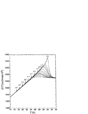
FIG. 1.: Total specific heat of an untwined YBa₂Cu₃O_7-δ single crystal with $T_{c}=91.87$ K for $H_{c}=H\|c$. The numbers on top of the spike indicate the strength of the applied magnetic field and the location of the melting transition. Taken from Schilling et al.[12]

In Fig.1 we displayed the data of Schilling et al.[12] for the temperature dependence of the heat coefficient of a YBa₂Cu₃O_7-δ single crystal with $T_{c}=91.87$ K at various magnetic fields applied parallel to the c-axis ($H_{c}$). As a remnant of the zero field singularity, there is for fixed field strength a broad peak adopting its maximum at $T_{p}$ which is located below $T_{c}$. As $T_{p}$ approaches $T_{c}$, the peak becomes sharper with decreasing $H$ and evolves smoothly to the zero-field singularity, smeared by the inhomogeneity induced finite size effect. The spike at $T_{m}<T_{p}$ is due to the melting transition[12]. Since $T_{p}$ increases systematically with increasing field, condition (33) is satisfied and there is a magnetic field induced finite size effect. Accordingly Eq.(37) for the field dependence of the relative shift should apply as long as 3D critical fluctuations dominate. In Fig.2 we displayed $t_{p}$ versus $H$ for the data shown in Fig.1. The solid line is Eq.(37) with

$$\left|t_{p}\right|=0.012\ H_{c}^{1/2\nu},$$ (39)

$H$ in T and $\nu$ given by Eq.(16). In the low field regime, where this asymptotic form applies it describes the data remarkably well, while for $\left|t_{p}\right|\gtrsim 0.04$ deviations pointing to corrections to scaling become manifest. To fix the universal constant $a$ entering Eq.(23) we use for $\xi_{0c}^{T}$ the estimate $\xi_{0c}^{T}=\sqrt{\xi_{a0}^{-}\xi_{b0}^{-}}=\sqrt{12.4\cdot 14.7}=13.5$A, derived from magnetic torque measurements[18], Eqs.(37) and (39) then yield for the universal constant $a$ entering the limiting length scales the estimate

$$a\approx 3.12.$$ (40)

In ⁴He this value leads with $L_{\Omega}=\sqrt{h/\left(2am_{4}\Omega\right)}$ and $\Omega=\left(2\pi\right)^{-1}$s^-1 to $L_{\Omega}\approx 5$ $10^{-2}$cm, which compares reasonably well with $5$ $10^{-2}$cm, the estimate derived by Haussmann[6]. Since at the lowest attained magnetic field, $H_{c}=1$T, (see Fig.1) a shift from $T_{c}$ to $T_{p}$ occurs, Eq.(37) yields for the inhomogeneities in the ab–plane the lower bound $L_{ab}>257A$, which is close to the estimates derived from the finite size effect in the zero field specific heat coefficient of untwined YBa₂Cu₃O_7-δ single crystals [18, 20].

FIG. 2.: (a)$\left|t_{p}\right|$ versus $H_{c}$ for the data shown in Fig.1. The solid line is Eq.(39) with $\nu$ listed in Eq.(16). (b) Melting line $T_{m}\left(H_{c}\right)$ in terms of $\left|t_{m}\right|$versus $H_{c}$ for the data shown in Fig.1. The solid line is Eq.(41)

The existence of the first order melting transition of the vortex lattice, seen in Fig.1 in terms of the spikes with numbers on the top, implies that the scaling function $G_{3}^{-}(z)$ in the free energy density (Eq.(20)) exhibits at some universal value $z_{m}$ of its argument a smeared singularity. For a magnetic field applied along the c-axis the melting line is then given by Eq.(37). In Fig.2b we compare this prediction with the experimental melting line, derived from the data shown in Fig.1, in terms of the solid line, which is

$$\left|t_{m}\right|=0.029\ H_{c}^{1/2\nu}.$$ (41)

Together with $\xi_{0c}^{T}=13.5$A, the value used to estimate $a$ (Eq.(LABEL:Eq38)), we obtain for the universal value of $z_{m}$ the estimate

$$z_{m}\approx 0.1.$$ (42)

Since a limiting length scale, like $L_{H}$ $\propto H^{-1/2}$, leads also to a rounding of first-order transitions[28], the vortex melting transition is expected to become broader with increasing magnetic field. This behavior appears to be confirmed by the extended study of the vortex melting transition in YBa₂Cu₃O_7-δ single crystals of Roulin et al.[13].

FIG. 3.: $\left|t_{p}\right|$ versus $H$ for YBa₂Cu₃O_6.9 with $T_{c}=92.56$ K derived from the data of Roulin et al.[13]. (a) $\left|t_{p}\right|$ versus $H_{ab}$; (b) $\left|t_{p}\right|$ versus $H_{c}$. The solid lines are Eqs.(43) with $\nu$ listed in Eq.(16).

To explore variations between data and single crystals of different provenance we show in Fig.3 t_p versus $H_{ab}$ and $H_{c}$ for YBa₂Cu₃O_6.9 single crystal with $T_{c}=92.56$K derived from the data of Roulin et al.[13]. The solid lines are

$$\left|t_{p}\left(H_{ab}\right)\right|=0.0033\ H_{ab}^{1/2\nu},\ \left|t_{p}\left(H_{c}\right)\right|=0.0132\ H_{c}^{1/2\nu},$$ (43)

corresponding to Eq.(37) with $H$ in T and $\nu$ given by Eq.(16). They yield with $a=3.12$ (Eq.(40)) the estimates

$$\xi_{0ab}^{T}=5.7\text{A},\ \xi_{0c}^{T}=14.4\text{A, }V_{c}^{-}=\left(\xi_{0ab}^{T}\right)^{2}\xi_{0c}^{T}=469\text{A}^{3}$$ (44)

Since at the lowest attained fields $H_{c}=0.25$T and $H_{ab}=2$T a shift from $T_{c}$ to $T_{p}$ is still present, we derive from Eq.(34) for the length scales of the sample inhomogeneities the lower bounds

$$L_{ab}>515\text{A},\ \ \sqrt{L_{ab}L_{c}}>182\text{A}.$$ (45)

The reported specific heat data also revealed melting lines consistent with the scaling form (37), namely

$$\left|t_{m}\left(H_{ab}\right)\right|=0.008\ H_{ab}^{1/2\nu},\ \left|t_{m}\left(H_{c}\right)\right|=0.032\ H_{c}^{1/2\nu},$$ (46)

with $\nu=2/3$, which is close to the 3D-XY value (Eq.(16)). Together with the expressions for the $t_{p}\left(H_{i}\right)$ lines (Eq.(43)) we obtain for the universal ratio $\left|t_{p}\left(H_{i}\right)\right|/\left|t_{m}\left(H_{i}\right)\right|=\left(az_{m}\right)^{1/2\nu}$ (Eq.38)) the estimates, $\left|t_{p}\left(H_{ab}\right)\right|/\left|t_{m}\left(H_{ab}\right)\right|=0.41$ and $\left|t_{p}\left(H_{c}\right)\right|/\left|t_{m}\left(H_{c}\right)\right|=0.42$, which agree with $\left(az_{m}\right)^{1/2\nu}=\left(3.12\ 0.1\right)^{3/4}$, derived from the independent estimates for $a$ (Eq.(40) and $z_{m}$ (Eq.(42)).

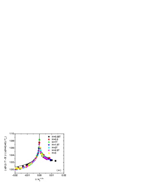
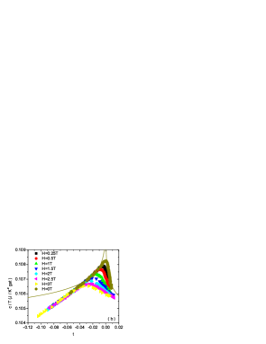
FIG. 4.: (a): $\left(c\left(T,H_{c}\right)/T-B^{-}\right)/\left(A^{-}\left|t\right|^{-\alpha}/\alpha\right)$ versus $t/H_{c}^{1/2\nu}$ for YBa₂Cu₃O_6.9 with $T_{c}=92.56$ K derived from the data of Roulin et al. [13], with $\alpha$ and $\nu$ given by Eq.(16), $\left(c\left(H,t\right)/T-B^{-}\right)$ in J/K²gat and $H$ in T. The values for $A^{-}/\alpha$ and $B^{-}$ are listed in Eq.(48). The solid line is Eq.(47); (b):  Specific heat coefficient $c/T$ versus $t$ of YBa₂Cu₃O_6.9 with $T_{c}=92.56$ K at various magnetic fields derived from the data of Roulin et al.[13]. The solid lines are Eq.(13) with $\alpha$ and $A^{+}/A^{-}$ given by Eq.(16) and the parameters listed in Eq.(48). The deviations of the zero field data from these lines reveal around $t=0$ the finite size effect due to inhomogeneities.

As the data of Roulin et al.[13] are rather dense and extend close to zero field criticality, a more detailed finite size scaling analysis appears to be feasible. Using Eq.(35), it is seen from Fig.4a that data collapse is obtained over a rather wide range of the scaling variable. Indeed, finite size scaling requires the data to collapse on the universal curve $g\left(y\right)$ with $\ y=t\left(\Phi_{0}/\left(aH_{c}\left(\xi_{0c}^{T}\right)^{2}\right)\right)^{1/2\nu}$. Furthermore, scaling also requires that at $T_{p}$, where $y=y_{p}=-1$, and for $\pm y\rightarrow 0$, $g\left(-1\right)=1$ and $g\left(y\right)\propto\left|y\right|^{-\left|\alpha\right|}$ for $\alpha<0$ should hold, respectively. Using $\xi_{0c}^{T}=14.4$A (Eq.(44)), it is seen from Fig.4a that at $y_{p}$, where $\left|t\right|/H_{c}^{1/2}=-0.013$, the scaling function is close to $1$, as required. In addition, the solid line which is

$$\frac{c\left(T,H_{c}\right)/T-B^{-}}{\left(A^{-}\left|t\right|^{-\alpha}/\alpha\right)}=0.957\left(\frac{-t}{H_{c}^{1/2}}\right)^{\alpha},$$ (47)

also confirms the divergence of the scaling function at $\pm y=0$. To qualify the remarkable collapse of the data we note that the estimates for $\widetilde{A}^{-}=A^{-}/\alpha$ and $B^{-}$ have been derived from the zero field data displayed in Fig.4b. The solid line for $t<0$ is Eq.(13) with

$$\frac{A^{-}}{\alpha}=\widetilde{A}^{-}=-0.073\text{(J/K}^{2}\text{gat)},\ \ B^{-}=0.179\text{(J/K}^{2}\text{gat), }B^{+}=0.181\text{(J/K}^{2}\text{gat), }T_{c}=92.56\text{K}$$ (48)

and the critical exponent $\alpha$ listed in Eq.(16), to indicate the inhomogeneity induced deviations from the leading zero field critical behavior of  perfect YBa₂Cu₃O_6.9. Since the data collapse onto the universal finite scaling function has been achieved without any arbitrary fitting parameter, the consistency with the magnetic field induced finite size scenario is well confirmed. Furthermore, Fig.4b shows how the broad anomaly in the specific heat coefficient sharpens and that the maximum height at $T_{p}\left(H_{c}\right)$ increases, evolving smoothly to the zero field peak, rounded by inhomogeneities.

To estimate the correlation volume from the specific heat coefficient in terms of the universal relation Eq.(15) we note that $A^{-}=T_{c}\alpha$ $\widetilde{A}^{-}$, $A^{-}$(cm^-3)$=\left(10^{4}/k_{B}/V_{gat}\right)A^{-}$(mJ/K/cm³) and $V_{gat}=8$cm³ give $A^{-}=7.96\ 10^{-4}$A^-3, yielding with $R^{-}=0.815$ (Eq.(16)) the correlation volume $V_{c}^{-}\approx 680$A³, which is reasonably close to the value derived from the magnetic field induced finite size effect (Eq.(44)). As in zero field the correlation volume $V_{c}^{-}\left|t_{p}\right|^{-3\nu}$ cannot grow beyond the volume $V_{i}$ of the inhomogeneities, this limiting volume scale is obtained from

$$V_{i}=V_{c}^{-}\left|t_{p}\right|^{-3\nu}.$$ (49)

and $t_{p}$ evaluated in zero field. With $V_{c}^{-}=469$A³ (Eq.(44)) and $\left|t_{p}\right|=0.0025$ taken from Fig.4b, we obtain the estimates $V_{i}=7.5\ 10^{7}$A³ and $V_{i}^{1/3}=422$A which is consistent with the aforementioned lower bounds listed in Eq.(45).

Noting that the critical amplitudes, the anisotropy $\gamma$ $=\left(\xi_{ab0}^{T}/\xi_{c0}^{T}\right)^{1/2}$ and the length scale of the inhomogeneities depend on the dopant concentration[19] it is instructive to analyze the data of Junod et al. [17] for underdoped YBa₂Cu₃O_6.6 with $T_{c}=64.2$K and $\gamma\approx 20$[29]. In Fig.5 we displayed the data for $\left|t_{p}\right|$ versus $H_{c}$ together with

$$\left|t_{p}\left(H_{c}\right)\right|=0.045\ H_{c}^{1/2\nu},$$ (50)

corresponding to Eq.(37) with $H$ in T and $\nu$ given by Eq.(16). It yields with $a=3.12$ (Eq.(40)) the estimate

$$\xi_{0c}^{T}=32.6\text{A,}$$ (51)

compared to $\ \xi_{0c}^{T}=14.4$ A (Eq.(44)) obtained close to optimum doping. Thus, the critical amplitude of  the correlation length $\xi_{0c}^{T}$ increases in the underdoped regime, reflecting the approach to the 2D quantum superconductor to insulator transition in the underdoped limit, where $\gamma$ tends to infinity[18, 19]. Typically, the leading scaling behavior becomes valid when $\left|t\right|$ becomes small and $H$ is small. However, one needs to know: How small is small enough? As there are corrections to the leading scaling behavior we know, when $\left|t\right|$ is no longer small, the temperature dependence of the transverse correlation length scales as[15, 16, 18]

$$\xi_{c}^{T}\left(t\right)=\xi_{0c}^{T}\left|t\right|^{-\nu}\left(1+a_{\xi_{c}^{T}}\left|t\right|^{\omega\nu}+..\right)$$ (52)

where $\omega\nu$ is the correction to scaling exponent, adopting in the 3D-XY universality class the value[16]

$$\omega\nu=0.53.$$ (53)

The dimensionless correction amplitude $a_{\xi^{T}}\$will in general become larger near a crossover. As YBa₂Cu₃O_7-δ undergoes with reduced oxygen concentration a 3D-2D crossover, $a_{\xi_{c}^{T}}$ is expected to increase, while the critical regime where the leading term dominates shrinks. To substantiate this expectation and to illustrate the effect of the corrections to scaling, we set  $\xi_{c}^{T}\left(T,H\right)=L_{H_{c}}$, to obtain with Eqs.(31) and (32) for $H_{c}\left(t_{p}\right)$ the expression

$$H_{c}\left(t_{p}\right)=\frac{\Phi_{0}}{a\left(\xi_{0c}^{T}\right)^{2}}\left|t_{p}\right|^{2\nu}\left(1+a_{\xi_{c}^{T}}\left|t_{p}\right|^{\omega\nu}\right)^{-2}.$$ (54)

A fit to the experimental data shown in Fig.5b yields

$$H_{c}=33.97\left|t_{p}\right|^{2\nu}\left(1-1.61\left|t_{p}\right|^{\omega\nu}\right)^{-2},$$ (55)

with $\nu$ and $\omega\nu$ given by Eqs.(16) and (53), respectively. This gives $\xi_{0c}^{T}=40.86$A which is considerably larger than $\xi_{0c}^{T}=32.6$A, the value derived without the correction to scaling. On the contrary, a fit to the data displayed in Fig.3b yields $H_{c}=319.66\left|t_{p}\right|^{2\nu}\left(1-0.014\left|t_{p}\right|^{\omega\nu}\right)^{-2}$, revealing that close to optimum doping the correction is up to $\left|t_{p}\right|=0.04$ negligibly small, while in the underdoped sample it is significant down to $\left|t_{p}\right|=0.02$. This confirms the expectation whereupon the 3D-2D crossover in the underdoped regime enhances the correction to scaling and reduces the critical regime where the leading scaling term dominates. From the data of Junod et al. [17] we also deduce that at the lowest attained field, $H_{c}=0.2$T, a shift from $T_{c}$ to $T_{p}$ occurs. This yields with Eq.(34) the lower bound

$$\sqrt{L_{a}L_{b}}>576\text{A}$$ (56)

compared to $515$ A, the value close to optimum doping (Eq.(45)).

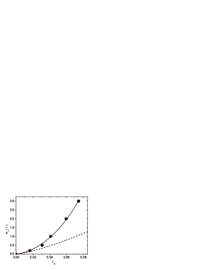
FIG. 5.: (a) $\left|t_{p}\right|$ versus $H_{c}$ for YBa₂Cu₃O_6.6 with $T_{c}=64.2$K derived from the data of Junod et al.[17]. The solid line is Eq.(47) with $\nu$ listed in Eq.(16). (b) $H_{c}$ versus  $\left|t_{p}\right|$ of the same data. The solid curve is Eq.(55) which takes the correction to the leading scaling term, $H_{c}=33.97\left|t_{p}\right|^{2\nu}$, displayed by the dashed line, into account.

Next we turn to Nb₇₇Zr₂₃[5], 2H-NbSe₂[4] and MgB₂[3], type II superconductors supposed to have comparative large correlation volumes. In Fig.6 we displayed $\left|t_{p}\right|$ versus $H$ derived from the respective experimental data. In contrast to the corresponding plot for nearly optimally YBa₂Cu₃O_7-δ (Fig.3), the data points to a linear relationship. Consequently, the critical regime, where $\left|t_{p}\right|$ $\propto$ $H^{1/2\nu\text{ }}$with $\nu\approx 2/3$ holds (Eq.(37)), is not attained. Nevertheless, there is clear evidence for a magnetic field induced finite size effect, because $T_{p}$ shifts monotonically to a lower value with increasing magnetic field. Since the data points to an effective critical exponent $\nu\approx 1/2$ which applies over an unexpectedly extended range, we use Eq.(37) with $\nu=1/2$ to derive estimates for the amplitude of the respective transverse correlation lengths and the correlation volume in terms of

$$\left|t_{p}\right|=b_{i}H_{i}=\frac{\left(\xi_{0i}^{T}\right)^{2}}{L_{H_{i}}^{2}}=\frac{aH_{i}\left(\xi_{0i}^{T}\right)^{2}}{\Phi_{0}},$$ (57)

with $a=3.12$ (Eq.(40). The respective straight lines in Fig.6 are this relation with the parameters listed in Table I. For comparison we included the corresponding parameters for YBa₂Cu₃O_6.9 and YBa₂Cu₃O_6.6 where the critical regime is attained. It is evident that Nb₇₇Zr₂₃, 2H-NbSe and MgB₂ are type II superconductors with comparatively large correlation lengths. Compared to YBa₂Cu₃O_6.9 and YBa₂Cu₃O_6.6 the correlation volume is 3 orders of magnitude larger, which renders the amplitude of the specific heat singularity very weak (see Eq.(13). Nevertheless, the unambiguous evidence for the magnetic field induced finite size effect reveals that fluctuations, even though not critical, are at work. For this reason there is no critical line $T_{c2}\left(H\right)$ of continuous phase transitions, but a line $T_{p}\left(H\right)$ where the specific heat peak, broadening and decreasing with increasing field, adopts its maximum value and the correlation length attains the limiting magnetic length scale $L_{H}$. Because the fluctuations are also subject to the finite size effect arising from inhomogeneities with length scale $L$, the magnetic finite size effect is observable as long as $L>L_{H}$. The resulting lower bounds for the length scale of inhomogeneities affecting the thermodynamic properties are also included in Table I. Noting that these bounds stem from studies where no attempt was made to explore the low field behavior, it is conceivable that the actual length scale of the inhomogeneities is much larger. To our best knowledge, the only absolute reference stems from the finite size scaling analysis of the zero field specific heat data of nearly optimally doped YBa₂Cu₃O_7-δ, where $L$ was found to range from $290$ to $419$A [20, 18]. Interestingly enough, the largest bound found here applies to the cubic superconducting alloy Nb₇₇Zr₂₃. In any case, the lower bounds ranging from $182$ to $814$A raise serious doubts on the relevance of the nanoscale spatial variations in the electronic characteristics observed in underdoped Bi-2212 with scanning tunnelling microscopy[21, 22, 23, 24].

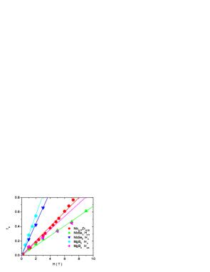
FIG. 6.: $\left|t_{p}\right|$ versus $H$ for Nb₇₇Zr₂₃[5], 2H-NbSe₂[4] and MgB₂[3] derived from the respective references. The straight lines are Eq.(57) with the parameters listed in Table I.

	$T_{c}$(K)	$b,b_{ab}$	$b_{c}$	$\xi_{0}^{T},\ \xi_{0ab}^{T}$(A)	$\xi_{0c}^{T}$(A)	V${}_{c}^{-}$(A3)	$L,\ L_{ab}$(A)	$\sqrt{L_{ab}L_{c}}$(A)
Nb77Zr23	$10.79$	$0.1$	$-$	$55.1$	$-$	$1.7\ 10^{5}$	$>814$	$-$
2H-NbSe2	$7.1$	$0.068$	$0.22$	$42.91$	$93.87$	$1.7\ 10^{5}$	$>258$	$>258$
MgB2	$35$	$0.09$	$0.28$	$51.73$	$110.24$	$2.9\ 10^{5}$	$>364$	$>258$
YBa2Cu3O6.95	$92.56$	$0.0033$	$0.0132$	$5.7$	$14.4$	$4.7\ 10^{2}$	$>515$	$>182$
YBa2Cu3O6.6	$64.2$	$-$	$0.045$	$-$	$32.6$	$-$	$>576$	$-$

Table I: Summary of the estimates for the transverse correlation length amplitudes, correlation volume $V_{c}=\left(\xi_{0ab}^{T}\right)^{2}\xi_{0c}^{T}$, lower bounds for the length scales $L_{ab}$ and $\sqrt{L_{ab}L_{c}}$ of inhomogeneities, derived from the magnetic field induced finite size effect. For Nb₇₇Zr₂₃, 2H-NbSe₂ and MgB₂ we used Eq.(57), describing the intermediate critical behavior displayed in Fig.6. Using the fact that at the lowest attained magnetic fields, $H=0.1$T (Nb₇₇Zr₂₃) [5], $H_{ab}=H_{c}=1$T (2H-NbSe₂) [4] and $H_{ab}=1$T, $H_{c}=0.5$T (MgB₂)[3], a shift from $T_{c}$ to $T_{p}$ was observed, we obtain with Eq.(34) the quoted lower bounds for the length scale of the inhomogeneities which affect the thermodynamic properties. For YBa₂Cu₃O_7-δ the estimates stem from the critical behavior shown in Figs.3 and 5, quoted in Eqs.(43), (44), (50) and (51), and the lower bounds are Eqs.(45) and (56).

The occurrence of fluctuations in type II superconductors with comparatively large correlation lengths also implies a rounding of the specific heat peak in zero field, where inhomogeneities set the limiting length scale. Such a rounding was found in the specific heat data of polycrystalline Mg¹¹B₂, obtained with high resolution ac calorimetry[39]. Further evidence for the relevance of fluctuations can be deduced from the specific heat coefficient at $T_{p}$. In Fig.7 we show the experimental data for Nb₇₇Zr₂₃[5]. For comparison we included Eq.(2) in the form

$$\frac{\Delta c\left(H,T_{p}\right)}{T_{p}}=c\left(1-bH\right)$$ (58)

with the parameters

$$c=18.1\text{mJ/K}^{2}\text{gat, \ \ }b=0.12\text{T}^{-1}.$$ (59)

Here fluctuations enter via the coefficient $b$ (Eq.(57)). For $H>0.2$T the data is consistent with a linear relationship and the coefficient $b$ derived from the field dependence of $T_{p}$ (see Table I). The difference between the zero field value $\Delta c\left(H=0,T_{c}\right)/T_{c}c=21$mJ/K²gat and the limit $\Delta c\left(H\rightarrow 0,T_{p}\right)/T_{p}$ $=c=18.1$mJ/K²gat is due to the triangular vortex lattice, for which the ratio between these coefficients should be $1.16$[2, 5].

FIG. 7.: $\Delta c\left(H,T_{p}\right)/T_{p}$ versus $H$ for Nb₇₇Zr₂₃. Experimental data taken from Mirmelstein et al.[5]. The solid line is Eq.(2) rewritten in the form (58) and the parameters listed in Eq.(59).

Although we concentrated hitherto on the specific heat, it should be kept in mind that the magnetic field induced finite size effect also affects other thermodynamic and the transport properties, including the magnetoconductivity. As an example we consider the linear magentoconductivity of a bulk sample. In the isotropic case the fluctuation contribution scales in zero field as $\sigma\propto\left(\xi^{T}\right)^{z-1}$[18], where $z$ is the dynamic critical exponent. Together with the evidence for static 3D-XY critical exponents there is mounting evidence for $z=2$ [18, 30, 40, 41] deduced from zero field data of the fluctuation contribution to the conductivity. In the presence of a magnetic field we obtain from Eq.(28) the scaling form

$$\sigma\propto\left(\xi^{T}\right)^{z-1}F(y),\text{ \ }y=\frac{aH\left(\xi^{T}\right)^{2}}{\Phi_{0}}=\left(\frac{\xi^{T}}{L_{H}}\right)^{2}$$ (60)

where $F(y)$ is a universal scaling function of its argument Since in an applied field the correlation length cannot grow beyond $L_{H}$, there is at $T_{p}$ the residual conductivity

$$\sigma\left(H_{p}\right)\propto\left(\frac{\Phi_{0}}{aH_{p}}\right)^{\left(z-1\right)/2}F(1),$$ (61)

where, using Eq.(23),

$$H_{p}\left(T\right)=\frac{\Phi_{0}}{a\xi_{0}^{2}}t^{2\nu}=\frac{\Phi_{0}}{a\xi_{0}^{2}}\left(1-\frac{T}{T_{c}}\right)^{2\nu},$$ (62)

This implies that type II superconductors in a magnetic field do not undergo a phase transition to a state with zero resistance. In particular there is no resistive upper critical field $H_{c2}\left(T\right)$. It is replaced by the line $H_{p}\left(T\right)$ where the resistivity attains the residual value $\rho\left(H_{p}\right)=1/\sigma\left(H_{p}\right)$. A characteristic feature is the positive curvature, $d^{2}H_{p}\left(T\right)/dT^{2}>0$, for $\nu>1/2$. This anomalous behavior has been found in a variety of cuprate superconductors[42, 43] and close to $T_{c}$ the data appears to be consistent with $2\nu\approx 4/3$, the value for 3D-XY critical behavior (Eq.(16)).

To summarize, we have shown that in type II superconductors subject to a magnetic field the correlation lengths cannot grow beyond the magnetic length scale $L_{H}$. Invoking the finite size scaling theory and the scaling form of the of the scaling form of the free energy density of an anisotropic type II superconductor close to zero field criticality we determined $L_{H}$ and explored the resulting finite size effect. In contrast to its inhomogeneity induced counterpart, arising from inhomogeneities with length scale $L$, $L_{H}\propto H^{-1/2}$ can be varied continuously in terms of the magnetic field strength. Thus, as long as $L>L_{H}$ the magnetic field induced finite size effect is observable and allows to assess the importance of fluctuations, to extract critical point properties of the homogeneous system and to derive a lower bound for the length scale of inhomogeneities which affect thermodynamic properties. Our analysis of specific heat data for under- and optimally doped YBa₂Cu₃O_7-δ, where the critical regime is attained, revealed remarkable agreement with the finite size scaling scenario. On the other hand the existence of the limiting magnetic length scale does have even away from the regime where critical fluctuations dominate essential consequences. Since the correlation length $\xi^{T}$ cannot grow beyond $L_{H}$, there is no critical line $H_{c2}\left(T\right)$ retaining the continuous character of the zero field transition. To illustrate this point we considered MgB₂, 2H-NbSe₂ and Nb₇₇Zr₂₃, type II superconductors with comparatively large correlation lengths. Although the analyzed experimental data do not extend to the critical regime, we have shown that there is a magnetic field induced finite size effect and with that fluctuations at work. Furthermore, lower bounds for the inhomogeneities affecting the thermodynamic properties have been derived. Their length scales range from $182$ A to $814$ A. Since the available data does not extend to low fields, much larger values are conceivable. This raises serious doubts on the relevance of the nanoscale spatial variations in the electronic characteristics observed with scanning tunnelling microscopy[21, 22, 23, 24]. In any case, we have shown that the various predictions we have made here are experimentally verifiable. In particular, the analogy with finite size scaling is robust and it should be possible to determine in exactly what regions the data collapses onto a one-variable scaling formulation and to what extent corrections to scaling can describe any deviations. Furthermore, in spite of the consensus that in type II superconductors in an applied magnetic field a phase transition to a state of zero resistance should occur, we have shown that the magnetic finite size effect points to the opposite conclusion. This is in agreement with the work reported in Refs.[25] and [26].

We thank H. Angst, H. Keller and C. Meingast for useful comments and suggestions.

REFERENCES

- [1] F. J. Morin et al., Phys. Rev. Lett. 14, 419 (1974)
- [2] A. L. Fetter and P. C. Hohenberg, in: Superconductivity, Ed. R. D. Parks, Vol. 2, M. Dekker Inc. 1969
- [3] L. Lyard et al., cond-mat/020623
- [4] D. Sanchez, A. Junod, J. Muller, H. Berger and F. Levy, Physica B 204,167 (1995)
- [5] A. Mirmelstein, A. Junod, E. Walker, B. Revaz, Y.-Y. Genoud, and G. Triscone, J. Superconductivity 10, 527 (1997)
- [6] R. Haussmann, Phys. Rev. B 60, 12373 (1999)
- [7] P. A. Lee and S. R. Shenoy, Phys. Rev. Lett. 28, 1025 (1972)
- [8] D. J. Thouless, Phys. Rev. Lett.34, 946 (1975)
- [9] E. Brezin, A. Fujita and S. Hikami, Phys. Rev. Lett. 65, 1949 (1990)
- [10] S. Hikami and S. Fujita, Phys. Rev. B 41, 6379 (1990)
- [11] R. Lortz, Report FZKA 6750, Forschungszentrum Karlsruhe (2002)
- [12] A. Schilling et al., Phys. Rev. Lett. 78, 4833 (1997)
- [13] M. Roulin, A. Junod and E. Walker, Physica C 296, 137 (1998)
- [14] P. C. Hohenberg et al., Phys. Rev. B 13, 2986 (1976)
- [15] V. Privmanet al., in: Phase Transitions and Critical Phenomena, Ed. C. Domb and J. L. Lebowitz, Vol. 14, Academic Press, 1991
- [16] A. Peliasetto and E. Vicari, cond-mat/0012164
- [17] A. Junod, A. Erb and Ch. Renner, Physica C 317, 333 (1999)
- [18] T. Schneider and J. M. Singer, Phase Transition Approach To High Temperature Superconductivity, Imperial College Press, London, 2000
- [19] T. Schneider, cond-mat/0204236
- [20] T. Schneider and J. M. Singer, Physica C 341-348, 87 (2000)
- [21] J. Liu, J. Wan, A. Goldman, Y. Chang and P. Jiang, Phys. Rev.Lett. 67, 2195 (1991)
- [22] A. Chang, Z. Rong, Y. Ivanchenko, F. Lu and E. Wolf, Phys. Rev. B 46, 5692 (1992)
- [23] T. Cren et al.,Phys. Rev. Lett. 84, 147 (2000)
- [24] K. M. Lang et al., cond-mat/0112232
- [25] D. R. Strachan, M. C. Sullivan, P. Fournier, S. P. Pai, T. Venkatesan, and C. J. Lobb, Phys. Rev. Lett. 87, 67007 (2001)
- [26] D. R. Strachan, M. C. Sullivan, and C. J. Lobb, cond-mat/0206120
- [27] M. E. Fisher and M. N. Barber, Phys. Rev. Lett. 28, 1516 (1972); M. E. Fisher, Rev. Mod. Phys. 46, 597 (1974)
- [28] V. Privman, Finite size scaling and numerical simulation of statistical systems, World Scientific, Singapore, 1990
- [29] B. Janossy, D. Prost, S. Pekker and L. Fruchter, Physica C 181, 91 (1991)
- [30] T. Schneider and H. Keller, Int. J. Mod. Phys. B 8, 487 (1993)
- [31] A. B. Harris, J. Phys. C 7, 1671 (1974)
- [32] E. Schultka and E. Manousakis, Phys. Rev. Lett. 75, 2710 (1995)
- [33] E. Schultka and E. Manousakis, Phys. Rev. B 52, 7528 (1995)
- [34] T. Schneider, J. Hofer, M. Willemin, J. M. Singer and H. Keller, Eur. Phys. J., B 3, 413 (1998)
- [35] J. Hofer et al., Phys. Rev. B 62, 631 (2000)
- [36] I. D. Lawrie, Phys. Rev. Lett. 79, 131 (1997)
- [37] X. Hu, S. Miyashita, and M. Tachiki, Phys. Rev. Lett. 79, 3498 (1997)
- [38] A. K. Nguyen and A. Sudbo, Phys. Rev. B 57, 3123 (1998)
- [39] T. Park et al., cond-mat/0204233
- [40] T. Schneider, G. I. Meijer, J. Perret, J.-P. Locquet and P. Martinoli, Phys. Rev. B 63, 144527 (2001)
- [41] K. D. Osborn et al., cond-mat/0204417
- [42] A. P. Mackenzie et al., Phys. Rev. Lett. 71,1238 (1993)
- [43] Y. Ando et al., Phys. Rev. B 60, 1475 (1999)