The segregation of sheared binary fluids in the Bray-Humayun model

Abstract

The phase separation process which follows a sudden quench inside the coexistence region is considered for a binary fluid subjected to an applied shear flow. This issue is studied in the framework of the convection-diffusion equation based on a Ginzburg-Landau free energy functional in the approximation scheme introduced by Bray and Humayun [Phys.Rev.Lett. 68, 1559, (1992)]. After an early stage where domains form and shear effects become effective the system enters a scaling regime where the typical domains sizes $L_{\parallel}$, $L_{\perp}$ along the flow and perpendicular to it grow as $t^{5/4}$ and $t^{1/4}$. The structure factor is characterized by the existence of four peaks, similarly to previous theoretical and experimental observations, and by exponential tails at large wavevectors.

I Introduction

The process of phase-separation occurring in binary systems quenched below the coexistence line has been matter of intensive investigations since many years. The overall phenomenology is nowadays reasonably well understood. In an early stage, whose properties depend on the system specific details, domains of the two phases form; the relative concentration of the two species well inside the domains quickly saturates to a value very similar to the equilibrium composition. Then a crossover leads to the late stage dynamics which is characterized by the growth of ordered regions of typical size $L(t)$ and by a statistically invariant morphology. This phenomenology is at the basis of the well known scaling property according to which a single length $L(t)$ is asymptotically relevant: system configurations at different times are simply related by a scale transformation with a scale factor $L(t)$. In particular, for the equal time density-density correlation function one has

$$G(\vec{r},t)=g\left[\frac{r}{L(t)}\right],$$ (1)

meaning precisely that $G$ is invariant as a function of scaled lengths $r/L(t)$. The growth of $L(t)$ is of the power law type $L(t)\sim t^{1/z}$. The dynamic exponent $z$ depends on the specific microscopic mechanisms responsible for the segregation process; in general different dynamical regimes can be observed, characterized by different values of $z$, by changing the experimental time window [1]. When the system enters the late stage the memory of the initial state is lost and, due to the presence of one single growing length, its properties become universal. Then the dynamical exponents, the scaling function $g$ and other observables become independent on the system specific details and are only determined by a few relevant parameters. Besides the spatial dimensionality, the presence of conservation laws is a relevant feature. For binary fluids, to which we restrict our attention, the concentration of the species is conserved as the phase-separation proceeds. The initial stage of the scaling regime, before hydrodynamic effects become relevant, is the subject of this paper. For viscous fluid this time window can be sufficiently wide to be detected experimentally. In this condition the phase-separation process is ruled by the evaporation, diffusion and subsequent recondensation of monomers [2] and the exponent $z$ is known to be $3$, independent on the space dimension $d$.

The spatial properties are encoded into the scaling function $g(x)$ or, equivalently, into its Fourier transform $f(q)$. For large $q$, $f$ has a power-law tail of the form $q^{-(d+1)}$: This is the famous Porod’s law [3], long recognized as arising from sharp domains walls.

Another relevant parameter affecting the scaling properties is the number of components $N$ of the order parameter $\phi$. For binary fluids $\phi$ is a scalar field. Most of the analytical techniques developed to study the kinetics, among which the Bray-Humayun scheme that is considered throughout this article, are however suited for vectorial systems with large-$N$. Let us briefly discuss the main features of vectorial systems that will be recalled in this paper. For systems with a continuous symmetry, rotations of the order parameter on the ${\cal O}(N)$ symmetric manifold of the local ground state of the Hamiltonian, instead of evaporation and condensation, is the important growth mechanism. This changes $z$ to $4$, regardless both of $d$ and $N$ (apart from exceptional cases [1]). Concerning the large-$q$ behavior of $f$ a generalization of the Porod’s law, $f(q)\sim q^{-(d+N)}$ is obeyed [4] for $N\leq d$. This form relies on the existence of stable localized topological defects. Much less is known about the tails of $f$ when these defects are not present, for $N>d$. Numerical simulations [5] found a stretched-exponential decay $f(q)\sim\exp[-q^{\nu}]$.

Despite this rather simple phenomenology the problem of deriving the scaling properties from first principles is still open. On the analytical side, the only soluble model [6] for conserved order parameter is the one with $N=\infty$. When considering this unphysical limit one hopes that the gross features of the kinetic process are retained for $N=\infty$ leaving further refinements to $1/N$ perturbation theories. However, although the global behavior of the $N=\infty$ model is qualitatively resemblant [7] of real systems, the scaling symmetry (1) is violated already at a qualitative level. The explicit solution of the model [6] shows in fact that instead of the standard scaling (1) one has a multiscaling symmetry produced by the existence of two logarithmically different lengths. Actually the ordering process with $N=\infty$ is more a condensation in momentum space [8], than a genuine phase-separation process. These results shadow the possibility to develop a successful theory of the segregation process by systematic $1/N$ expansions around the large-$N$ limit.

In this scenario a prominent role is played by a class of approximate theories known as gaussian auxiliary field theories, originally introduced by Mazenko [9]. The essence of these is a non-linear mapping between the order parameter $\phi(\vec{x},t)$ and an auxiliary field $m(\vec{x},t)$. The actual form of the relationship $m(\phi)$ is largely arbitrary and, depending on different physically motivated choices, different schemes have been developed [10]. The basic idea is that with a proper choice of $m(\phi)$ the equation obeyed by the auxiliary field can be treated to lowest order in a mean-field approximation while the basic non-linearities of the evolution are still retained through the non-linear mapping $m(\phi)$. This ad hoc assumption is generally uncontrolled and its use is justified a posteriori by the satisfactory quality of the predictions. Starting from the method of Mazenko, Bray and Humayun (BH) have derived [11] a non-linear closed equation of motion for the correlation function $G(\vec{r},t)$ within the framework of the $1/N$ perturbative expansion. Letting $N\to\infty$ in the BH equation one recovers the large-$N$ model previously discussed; the BH approach, however, does not amount to a straightforward $1/N$-expansion because all orders in $1/N$ are reintroduced through the gaussian auxiliary field approximation. On one side, the uncontrolled character is the limit of the BH scheme, since it is not clear how to improve the approximation, but on the other side, represents a powerful tool to overcome the shortcomings of standard perturbation theory previously discussed. As shown by BH their equation reinstates standard scaling (1) as a truly asymptotic symmetry, leaving to multiscaling a merely pre-asymptotic role. An additional feature at variance with the $N=\infty$ limit is the form of the scaling function $f(q)$, which, in the BH approximation falls exponentially at large momenta, as opposed to the quartic exponential decay of the $N=\infty$ model.

In this paper we are interested in the diffusive phase separation process of a binary fluid in the presence of an applied shear flow, namely an imposed fluid velocity along $x$ with a constant gradient along $y$. The presence of the flow radically changes the behavior and even the phenomenology is much less understood. A first trivial effect is the anisotropic deformation of the growing pattern that appears greatly elongated along $x$ [12, 13, 14, 15]. Then, when dealing with growth laws one has to specify the length of the equilibrated regions for each direction, $L_{x}(t),L_{y}(t),L_{z}(t)$, and in general $L_{x}(t)>>L_{y}(t),L_{z}(t)$. A more subtle point, that may have important consequences, is the following: stretching of the domains causes ruptures of the network [14] that may render the segregation incomplete. Actually, the characteristic lengths in the different directions could keep on growing indefinitely, as without shear, or due to domains break-up the system may eventually enter a stationary state characterized by domains with a finite thickness. In general there is no agreement on this point both from the experimental [15] and theoretical point of view. On the theoretical side large-$N$ calculations [16, 17] show the existence of a multiscaling regime with ever growing lengths in all directions. However numerical simulations [18] cannot still establish a clear evidence due to finite size and discretization effects. Another intriguing feature which is probably related to the stretching and break-up of the domains is the observation of an oscillatory pattern in the observables. Let us consider the excess viscosity $\Delta\eta$ as an example. Stretching of domains require work against surface tension leading to an increase of $\Delta\eta$. However when a domain breaks up the stress is released since the fragments are more isotropic; this produces a decrease of $\Delta\eta$. If repeated in time this mechanism produces an oscillatory pattern that is observed in simulations [18] and possibly in experiments [19]. In the large-$N$ limit it can be shown that this process has a periodicity in $\log t$. Similar patterns are also reported in apparently different contexts as fractures in heterogeneous solids [20] or in stock market indices [21], suggesting a possible common underlying interpretation. However we do not have nowadays analytical tools to enlighten this feature.

The spatial properties of the mixture are encoded into the correlation function $G(\vec{r},t)$ or, equivalently, into its Fourier transform $C(\vec{k},t)$, the structure factor. The latter is directly measured with scattering techniques and is more suited for comparison with the experiments. The form and the evolution of $C$ are themselves modified by the presence of the flow. When the shear becomes effective, after an initial isotropic regime where $C$ has the shape of a circular volcano, the tip of $C$ is deformed into an ellipses. This is expected as a consequence of the anisotropy, and is generally observed in experiments. In some cases the presence of four pronounced peaks on the edge of $C$ can be detected [22]. The existence of these multiple maxima has been also observed in numerical studies [18] of phase separation and in different physical systems such as stationary microemulsion in shear flow [23], suggesting that this is a rather general feature of sheared fluids. A peak in the structure factor is generally interpreted as the signature of a characteristic length proportional to the inverse of the wavevector where the peak is located. In this anisotropic case to each peak one associates one typical length for each space direction. Taking into account the symmetry $\vec{k}\to-\vec{k}$ this suggests that a couple of characteristic lengths for each direction is present: It is not completely clear, however, to which extent this interpretation can be pushed.

In this partly unclear scenario the development of theoretical tools for reliable predictions to be tested in experiments is important. In the case without shear the BH scheme turns out to be a reference theory capable to describe the main ingredients of the phenomenology. Therefore in this paper we address a numerical solution of the BH equation in the presence of shear flow. We will compare its behavior with previous results pertaining to the large-$N$ limit or to numerical simulations of the fully non-linear scalar model. Our results confirm the occurrence of a scaling regime with growing lengths in every direction. The dynamical exponents are found to coincide with those of the $N=\infty$ model. The four peak pattern for the structure factor is exhibited, similarly to what observed both for $N=\infty$ and in the scalar model, the actual form of $C$ being, however, rather different in the three cases. Concerning the oscillating behavior of the typical lengths and of the excess viscosity, on the other hand, the BH model behaves quite differently, in that these are strongly inhibited or even absent, at variance with $N=\infty$ and $N=1$.

This paper is divided in 4 Sections: In Sec. II we introduce the BH equation and discuss some numerical details about its integration; in Sec. III the results of the numerical solution are presented and a comparison with different approaches is proposed. In Sec. IV we draw the conclusions of this work.

II The model

We consider a system described by an order parameter with $N$ components. The evolution is described by the convection-diffusion equation [1] that generalizes the Cahn-Hilliard-Cook equation in the case of an applied velocity field $\vec{v}$

$$\frac{\partial{\bf\phi}(\vec{x},t)}{\partial t}+\vec{\nabla}\cdot\left[{\bf\phi}(\vec{x},t)\vec{v}(\vec{x},t)\right]=\Gamma\nabla^{2}\frac{\delta{\cal F}\left(\{{\bf\phi}\}\right)}{\delta{\bf\phi}}+{\bf\eta}(\vec{x},t)$$ (2)

where ${\bf\phi}\equiv\{\phi_{\alpha}\}$ is the vector order parameter that in the scalar case represents the concentration difference between the two species of the fluid, $\vec{x}\equiv\{x,y,z\}$ is the space coordinate, $\Gamma$ is a transport coefficient and ${\bf\eta}$ is a gaussian stochastic field with expectations

$$\langle{\bf\eta}(\vec{x},t)\rangle = 0$$ (3)

$$\langle{\bf\eta}(\vec{x},t){\bf\eta}(\vec{x}^{\prime},t^{\prime})\rangle = -2T\Gamma\nabla^{2}\delta(\vec{x}-\vec{x}^{\prime})\delta(t-t^{\prime})$$ (4)

describing thermal fluctuations. The symbol $\langle\dots\rangle$ means an ensemble average. ${\cal F}$ is the equilibrium Ginzburg-Landau free energy

$${\cal F}(\{{\bf\phi}\})=\int d\vec{x}\left[\frac{r}{2}{\bf\phi}^{2}+\frac{g}{4N}\left({\bf\phi}^{2}\right)^{2}+\frac{u}{2}|\nabla{\bf\phi}|^{2}\right]$$ (5)

where $\phi^{2}=\sum_{\alpha}\phi_{\alpha}\phi_{\alpha}$. The parameter $r$ distinguishes between the mixed state with $r>r_{c}(T)$ ($r_{c}(T)<0$) and the phase separated states with $r<r_{c}(T)$. For a plane shear flow the velocity term is given by

$$\vec{v}=\gamma y\vec{e}_{x}$$ (6)

where $\vec{e}_{x}$ is the unit vector in the flow direction $x$ and $\gamma$ is the shear rate.

In the approximation framework developed by BH [11] the following equation of motion can be derived for the equal time correlation function $G(\vec{r},t)=\langle\phi_{\alpha}(\vec{x},t)\phi_{\alpha}(\vec{x}+\vec{r},t)\rangle$

$$\frac{\partial G(\vec{r},t)}{\partial t}+\gamma y\frac{\partial G(\vec{r},t)}{\partial x}=-2\nabla^{2}\left\{\nabla^{2}G(\vec{r},t)-R(t)\left[G(\vec{r},t)+\frac{1}{N}G^{3}(\vec{r},t)\right]\right\}$$ (7)

where we have dropped the component indices due to internal symmetry. In deriving Eq. (7) from Eq. (2) we have let $\Gamma=1$ and $u=1$ since this simply amounts to a redefinition of time and space scales and we have neglected the thermal disturbance $\eta$ because it can be shown [24, 18] that the temperature is an irrelevant parameter below the coexistence line. The quantity $R(t)$ is a function of time that is asymptotically determined by the requirement $\lim_{t\to\infty}G(0,t)=S_{eq}=-r/g$. Here we use the self-consistent determination of $R(t)$

$$R(t)=g[G(0,t)-S_{eq}]$$ (8)

that is usually adopted [11, 25]. For $N=\infty$, namely dropping the cubic term on the r.h.s., Eq. (7) becomes the $N=\infty$ model.

We have considered the evolution of Eq. (7) with $N=1$. Some comments about the role of $N$ are in order. Eq. (7) is derived in an $1/N$ perturbative framework. Then, in principle, the quality of the approximation is expected to be better for large $N$ and, in any case, this whole approach is meaningful for vectorial systems with continuous symmetry. Given that the nature of the symmetry is relevant for the scaling properties, as discussed in Sec. I, one cannot pretend to push this scheme down to the physically relevant case with $N=1$ in a completely successful way. However, besides numerical simulation that are quite difficult and not particularly instructive in this case, most of the understanding of phase separation with shear comes nowadays from the $N=\infty$ model, which surely suffers of much more profound shortcomings than the present approach, if used to infer the properties of physical systems. The BH scheme represents a first step beyond $N=\infty$, despite of course being not conclusive. It must be recalled, moreover, that at least without shear the BH equation substantially reproduces the behavior of the system with $N=\infty$, including multiscaling, in a preasymptotic time domain $t<t^{*}(N)\sim(\Delta N)^{4/d}(\ln N)^{3}$ after which the cubic correction in Eq. (7) becomes effective [11]. The choice $N=1$, besides being appropriate for physical systems, is also the most efficient in order to amplify as much as possible the role of finite-$N$ corrections, given the limited timescale numerically accessible.

Eq. (7) have been solved on a two dimensional lattice of size $L=4096$, the lattice constant being $\Delta x=1$, via a finite difference first order Euler scheme with $\Delta t=0.01$. Periodic boundary conditions have been adopted. The initial condition $G(\vec{r},0)=\Delta\delta(\vec{r})$, $\Delta$ being a constant, corresponds to a quench from an equilibrium state at infinite temperature. The parameter of the free energy we use are $-r=g=1$; different choices correspond to a redefinition of the order parameter amplitude. We will present data relative to the case $\gamma=0.01$ and $\Delta=0.01$; we have tested that other choices produce similar results.

The structure factor $C(\vec{k},t)=\langle\hat{\phi}(\vec{k},t)\hat{\phi}(-\vec{k},t)\rangle$ obeys the equation

$$\frac{\partial C(\vec{k},t)}{\partial t}-\gamma k_{x}\frac{\partial C(\vec{k},t)}{\partial k_{y}}=-2k^{2}\left[k^{2}+R(t)\right]C(\vec{k},t)-2\frac{k^{2}}{N}R(t)D(\vec{k},t)$$ (9)

where $D(\vec{k},t)$ is the Fourier transform of $G^{3}(\vec{r},t)$. Due to the structure of this Equation, however, it is more efficient to compute $G$ from Eq. (7) and to obtain $C$ by Fourier transform. From the knowledge of $C$ one can extract the characteristic lengths along $x$ and $y$ as

$$L_{x}(t) = \left(\frac{\int d\vec{k}|k_{x}|C(\vec{k},t)}{\int d\vec{k}C(\vec{k},t)}\right)^{-1}$$ (10)

$$L_{y}(t) = \left(\frac{\int d\vec{k}|k_{y}|C(\vec{k},t)}{\int d\vec{k}C(\vec{k},t)}\right)^{-1}$$ (11)

and rheological indicators such as the shear stress

$$\sigma_{xy}(t)=\int\frac{d\vec{k}}{(2\pi)^{d}}k_{x}k_{y}C(\vec{k},t)$$ (12)

For a steady flow the excess viscosity is defined in terms of the shear stress as $\Delta\eta(t)=-\gamma^{-1}\sigma_{xy}(t)$.

III results

The anisotropic character of the evolution, with the ordered regions aligning along the flow direction, is reflected in the behavior of the correlation function $G$, shown in Fig. (1). $G$ has a peak at $\vec{r}=0$ and is continuously stretched along the $x$-direction, assumining increasingly eccentric elliptical patterns.

Snapshots of the structure factor at the same times are shown in the $k_{x},k_{y}$ plane in Fig. (2). Initially, not shown here, $C$ develops the form of a circular volcano, as in the case without shear. A later observation, at $\gamma t=1$, shows a deep in the volcano profile along the direction $k_{y}=-k_{x}$. This deep becomes progressively more pronounced until $C$ appears separated into two symmetric foils. At times of order $\gamma t=5$ in each foil a couple of maxima are built up. We denote by the letter A the peak that in the figure at time $\gamma t=5$ is higher. With respect to the other maximum, denoted by B, A is characterized by having $|k_{x}|>>|k_{y}|$, whereas in B $|k_{x}|\simeq|k_{y}|$. The relative height of these maxima changes in time. This is observable in Fig. (2) at time $\gamma t=9$: now B is prevailing.

Up to this time the qualitative evolution of the structure factor is comparable to what reported for $N=\infty$ [17] and for the numerical solution [18] of the full model equation with $N=1$. Computer limitations prevent the observation of the system on longer times. Only in the $N=\infty$ case the dynamics can be followed by numerical integration of the equations on larger timescales and it can be shown that the repeated prevalence of either A or B maxima continues cyclically in time. It turns also out that the recurrent dominance of A and B is periodic in the logarithm of the strain $\gamma t$. A physical interpretation of this pattern in terms of stretching and break-up of domains is proposed in [18].

The spherical average

$$C_{sf}(k,t)={\cal N}^{-1}\int d\theta C(\vec{k},t),$$ (13)

where $\tan\theta=k_{y}/k_{x}$ and ${\cal N}$ is the number of lattice points contained in a circular shell of width $\pi/256$ centered around $k$, and the averages along $k_{x}$ or $k_{y}$

$$C_{x}(k_{y},t)=L^{-1}\int dk_{x}C(\vec{k},t)$$ (14)

and

$$C_{y}(k_{x},t)=L^{-1}\int dk_{y}C(\vec{k},t)$$ (15)

are plotted in Fig. (3). This figure shows that in the large-$\vec{k}$ tail the structure factor decays exponentially, as already observed without imposed flow [25], at variance with the faster decay observed for $N=\infty$ [16]. As already mentioned, the absence of power-law tails is related to the absence of stable localized topological defects in the Bray-Humayun approximation.

Next we consider the growth laws. For $N=\infty$, in the large time region [16, 17] $L_{x}$ and $L_{y}$ keep increasing with (logarithmically corrected) power laws $L_{x}\sim\gamma(t^{5}/\ln t)^{1/4}$, $L_{y}\sim(t/\ln t)^{1/4}$ modulated by a log-periodic oscillation. The short time part of this pattern is observed in Fig. (4b). The same growth exponents are expected for the BH model (but without logarithmic corrections); this is because the model amounts to an $1/N$ perturbative expansion and, therefore, it is accurate for vectorial systems whose growth exponents belong to the same universality class of $N=\infty$. Actually the value of the exponents can be easily determined by means of a scaling analysis. If standard scaling holds the structure factor can be cast as

$$C(\vec{k},t)=L_{x}(t)L_{y}(t)f(X,Y)$$ (16)

where $X=k_{x}L_{x}(t)$ and $Y=k_{y}L_{y}(t)$ and $f$ is a scaling function. From (16) one also has

$$D(\vec{k},t)=bL_{x}(t)L_{y}(t)h(X,Y)$$ (17)

where $b$ is a constant and $h$ another scaling function. Inserting expressions (16,17) into the equation of motion of $C$ (9) and assuming that asymptotically $L_{x}$ prevails over $L_{y}$ one obtains

$$2Y^{4}f(X,Y) = -2R(t)L_{y}(t)^{2}\left[f(X,Y)+\frac{b}{N}h(X,Y)\right]Y^{2}+\frac{L_{y}(t)^{5}}{L_{x}(t)}\gamma X\frac{\partial f(X,Y)}{\partial Y}$$ (18)

$$- \frac{1}{4}\frac{dL_{y}(t)^{4}}{dt}\left\{1+\frac{\frac{d\left[\ln L_{x}(t)\right]}{dt}}{\frac{d\left[\ln L_{y}(t)\right]}{dt}}\right\}$$ (19)

The l.h.s. of Eq. (19) does not depend explicitly either on time and $\gamma$. Then in order to fulfill this equation for each $X,Y$ both $t$ and $\gamma$ must drop out from the r.h.s. Then one has

$$\left\{\begin{array}[]{ll}L_{x}(t)\sim\gamma t^{\frac{5}{4}}\\ L_{y}(t)\sim t^{\frac{1}{4}}\\ R(t)\sim t^{-\frac{1}{2}}\end{array}\right.$$ (20)

As already anticipated the exponents are those pertaining to systems with continuous symmetry. Furthermore one can observe that the shear rate enters linearly in $L_{x}$ but the growth in the shear direction $y$ is unaffected by $\gamma$. For completeness we recall that in the full scalar model one expects different exponents, namely $L_{x}\sim\gamma t^{4/3}$, $L_{y}\sim t^{1/3}$ from scaling [16] or renormalization group [18] arguments, but these are not yet clearly observed in simulations. Moreover the very existence of an asymptotic scaling dynamics is debated in this case. Fig. (4a) shows that initially both $L_{x}$ and $L_{y}$ start growing with an exponent which is consistent with the value $1/4$ as in absence of shear. In this time regime the fluid essentially does not feel the presence of the flow, as already discussed for the structure factor. Then, starting from $\gamma t\simeq 0.5$, $L_{y}$ keeps growing unexpectedly larger than $L_{x}$ untill at $\gamma t\simeq 2$ it decreases. Up to this point the BH model roughly resembles the $N=\infty$ case, despite the fact that the overshoot of $L_{y}$ is much more pronounced in the latter case. Fig. (4c), instead, shows that the full scalar model behaves quite differently, with a pronounced decrease of $L_{y}$ in the range of times where in the other models a fast growth was observed. For longer times the asymptotic stage is entered. The numerical integration of the BH model presented insofar shows that Eq. (20) is obeyed but, at variance with the other two cases, the oscillatory pattern is absent or, at least, strongly depressed.

Now we turn to the discussion of Fig. (5) where the behavior of the excess viscosity is reported. In all the cases considered $\Delta\eta$ initially grows to a maximum, then falls negative and raises to a second maximum. This pattern has been observed also in experiments [19] and is referred to as double overshoot. After the second maximum the asymptotic stage is entered. On the basis of scaling arguments one expects that $\Delta\eta$ scales as $\gamma^{-1}$ times the inverse of the typical volume $L_{x}L_{y}$ of the domains of the two species. Then $\Delta\eta\sim\gamma^{-2}t^{-3/2}$ for vector order parameter and $\Delta\eta\sim\gamma^{-2}t^{-5/3}$ for the scalar model. The former exponent is observed in Fig. (5a) for the BH model, although in the very last part of the simulation. For $N=\infty$ the same exponent (with logarithmic corrections) has been exactly computed [16] and observed numerically on larger timescales, but modulated by log-time periodic oscillations [17]. In the scalar case a definite exponent cannot be extracted from simulations, but the oscillations are observed.

IV conclusions

In this Article we have considered the behavior of a binary fluid quenched below the mixing temperature in the presence of an applied shear flow. The description of this system has been carried out in the context of the continuum convection-diffusion equation based on the Ginzburg-Landau equilibrium free energy. The nature of our approach, which neglects hydrodynamic effects, limits the domain of applicability of the model to the diffusive regime which takes place at short times. We have studied this model in the approximation scheme introduced by Bray and Humayun. This amounts to an expansion in $1/N$ on top of the auxiliary field theory approximation originally introduced by Mazenko. A comparison is also presented with two different approaches: the $N=\infty$ limit and the full scalar model, which is the most appropriate for fluids. The first has the great advantage to be fully soluble analytically, al least in the large time domain, providing an unambiguous description. Furthermore it can be easily studied numerically from the instant of the quench onwards. However, besides the fact that the case $N=\infty$ is far from physical, it has also proved to violate the qualitative symmetry of standard scaling in favor of multiscaling, rendering this model insecure as an approximation to real systems. On the other hand the full scalar model is well suited for describing fluids but it cannot be studied analytically. Numerical simulations, although important, have not yet provided clear evidences of the basic phenomenology, due to technical limitations. The BH model is ideally located in between these two: It shares with the large-$N$ limit the property of being a closed equation for an observable, the correlation function, that is already an ensemble average. Then, even if one resorts in the end to a numerical solution, one still has the great advantage to avoid the average over a large number of realizations. Secondly, due to its perturbative character, it is believed to represent a step forward with respect to the case $N=\infty$. This statement has been proven to be correct at least without shear.

Given the essence of the BH scheme, one does not expect to obtain a fully reliable approximation to real systems with $N=1$. The spirit of this work is more to establish if and to which extent its phenomenology compares better to the numerical simulations of the physical model than to the case $N=\infty$. From the analysis of the behavior of the characteristic lengths and of the excess viscosity we can conclude that the BH model behaves more like the $N=\infty$ case with damped oscillations than like the full scalar model, despite that, with the choice $N=1$, the corrections to the case $N=\infty$ contained in Eq. (7) are effective almost from the beginning, as it is clear from Figs. (4,5). This is true not only for the value of the dynamic exponents, but also for the qualitative behavior of the typical lengths.

On the other hand, regarding the oscillating character of most observables, the BH model behaves rather differently from both $N=\infty$ and $N=1$ in that strong oscillations are observed in the latter two while they are practically absent in the former. Under this respect the BH model is atypical and cannot be regarded as a bridge between $N=\infty$ and $N=1$. It is possible that the BH scheme resembles more the behavior of vectorial system with a finite $N$ under shear, but this is a totally unexplored field.

Regarding the important issue of the existence of an asymptotic scaling regime characterized by ever growing lengths $L_{x},L_{y}$, in the time range accessed in this work we do not see any saturation effect and both $L_{x}$ and $L_{y}$ keep firmly growing with the expected power laws. In the BH scheme, then, the presence of an asymptotic scaling regime is confirmed while a stationary state with domains of a finite thickness is not observed.

Acknowledgments

We warmly acknowledge Marco Zannetti for suggesting this study. F.C. and G.G. acknowledge partial support by the European TMR Network-Fractals Contract No. FMRXCT980183 and by INFM PRA-HOP 1999.

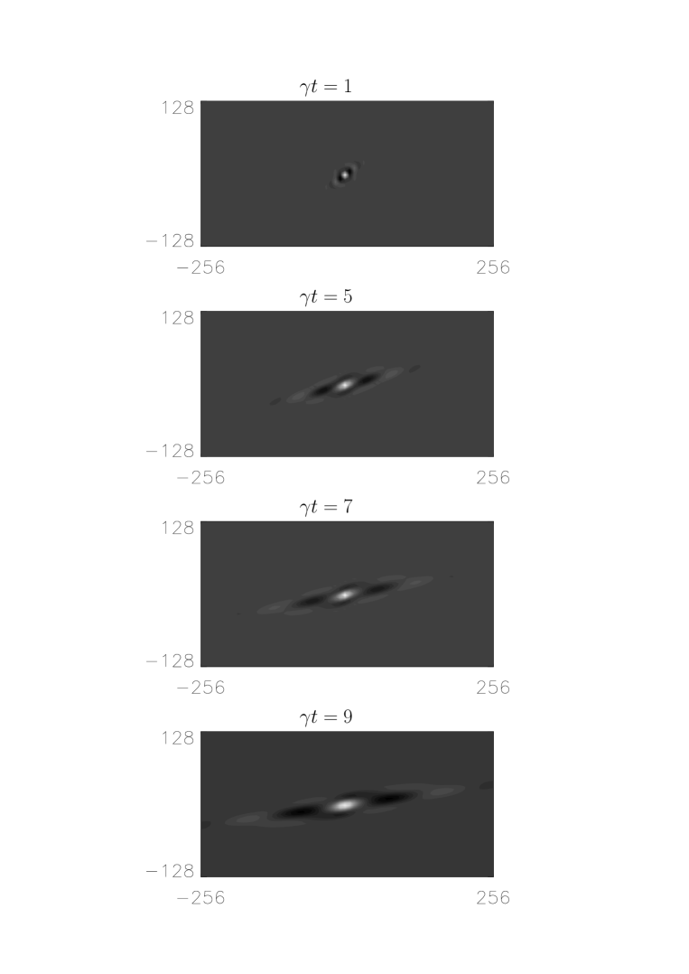
FIG. 1.: The real-space correlation function $G(\vec{r},t)$ is shown (only a part of the whole lattice) at four different values of the strain, $\gamma t=1,5,7,9$. $x$ is on the horizontal axis.

FIG. 2.: The structure factor $C(\vec{k},t)$ is shown at four different values of the strain, $\gamma t=1,5,7,9$. $k_{x}$, on the horizontal axis, increases from left to right; $ky$ increases toward the back of the figure.

FIG. 3.: The structure factors averaged along the $k_{x}$ and $k_{y}$ directions and spherically are shown for $\gamma t=10$ ($\bullet$), 15 ($\ast$), 20 ($\triangle$), 25 ($\circ$) and 30 ($\star$).

FIG. 4.: The evolution of the characteristic lengths $L_{x}(t),L_{y}(t)$ is shown for a) the BH model, b) the $N=\infty$ limit, c) the full scalar model (numerical simulation). In a) and b) the straight lines represent the expected power law behaviors $L_{x}(t)\sim t^{5/4}$, $L_{y}(t)\sim t^{1/4}$.

FIG. 5.: The evolution of the excess viscosity $\Delta\eta(t)$ is shown for a) the BH model, b) the $N=\infty$ limit, c) the full scalar model (numerical simulation). The straight lines represent the power law behavior $\Delta\eta(t)\sim t^{-3/2}$.

REFERENCES

- [1] A.J. Bray Adv. Phys. 43, 357, (1994); J.D. Gunton, M. San Miguel and P.S. Sahni, in Phase Transitions and Critical Phenomena, edited by C. Domb and J.L. Lebowitz (Academic Press, London 1983), Vol.8.
- [2] I.M. Lifshitz and V.V. Slyozov, J. Phys. Chem. Solids 19, 35 (1961); C. Wagner, Z. Elettrochem. 65, 581, (1961).
- [3] G. Porod, in Small-Angle X-ray Scattering, edited by O. Glatter and O. Kratky (Academic, London, 1983).
- [4] A.J. Bray and S. Puri, Phys. Rev. Lett. 67, 2670 (1991); H. Toyoki, Phys. Rev. B 45, 1965 (1992).
- [5] M. Rao and A. Chakrabarti, Phys. Rev. E 49, 3727 (1994).
- [6] A. Coniglio and M. Zannetti, Europys. Lett. 10 , 575, (1989).
- [7] A. Coniglio, P. Ruggiero and M. Zannetti Phys. Rev. E 50, 1046 (1994); U. Marini Bettolo Marconi and F. Corberi, Europhys. Lett. 30, 349, (1995); S. Glotzer and A. Coniglio, Phys. Rev. E 50, 4241, (1994); F. Corberi and C. Castellano, phys. Rev. E 58, 4658 (1998); C. Castellano and F. Corberi, Phys. Rev. E 57, 672 (1998).
- [8] C. Castellano, F. Corberi and M. Zannetti Phys. Rev. E 56, 4973 (1997).
- [9] G.F. Mazenko, Phys. Rev. Lett. 63, 1605 (1989); Phys. Rev. B 42, 4487 (1990); 43, 5747 (1990).
- [10] C. Yeung, Y. Oono and A.Shinozaki, Phys. Rev. E 49, 2693, (1994); S. De Siena and M. Zannetti, Phys. Rev. E 50, 2621, (1994); T. Otha, D. Jasnow and K. Kawasaky, Phys. Rev. Lett. 49, 1223, (1982); A.J. Bray and K. Humayun, Phys. Rev. E 48, R1609 (1993).
- [11] A.J. Bray and K. Humayun, Phys.Rev.Lett. 68, 1559, (1992).
- [12] For a review, see A. Onuki, J. Phys: Condens. Matter. 9, 6119, (1997).
- [13] D.H. Rothman, Europhys. Lett. 14, 337, (1991); K. Matsuzaka, T. Koga and T. Hashimoto, Phys. Rev. Lett. 80, 5441, (1998).
- [14] T. Otha, H. Nozaki and M. Doi, Phys. Lett. A 145, 304, (1990).
- [15] T. Hashimoto, K. Matsuzaka, E. Moses and A. Onuki, Phys. Rev. Lett. 74, 126, (1995); T. Takebe, F. Fujioka, R. Sawaoka and T. Hashimoto, J. Chem. Phys. 98, 717, (1993); J. Läuger, C. Laubner and W. Gronsky, Phys. Rev. Lett. 75, 3576, (1995); C.K. Chan, F. Perrot and D. Beysens, Phys. Rev. A 43, 1826, (1991).
- [16] N.P. Rapapa and A.J. Bray, Phys. Rev. Lett. 83, 3856, (1999).
- [17] F. Corberi, G. Gonnella and A. Lamura, Phys. Rev. Lett. 81, 3852, (1998); F. Corberi, G. Gonnella and A. Lamura, Phys. Rev. E 61, 6621, (2000).
- [18] F. Corberi, G. Gonnella and A. Lamura, Phys. Rev. Lett. 83, 4057, (1999); F. Corberi, G. Gonnella and A. Lamura, Phys. Rev. E 62, 8064, (2000).
- [19] Z. Laufer, H.L. Jalink and A.J. Staverman, Journal of Polymer Science 11, 3005, (1973); S. Mani, M.F. Malone, H.H. Winter, J.L. Halary and L. Monnerie, Macromolecules 24, 5451, (1991); S. Mani, M.F. Malone and H.H. Winter, Macromolecules 25, 5671, (1992).
- [20] M. Sahimi and S. Arbabi, Phys. Rev. Lett. 77, 3689, (1996); D. Sornette, Phys. Rep. 297, 239, (1998).
- [21] A. Johansen and D. Sornette, cond-mat/9907270.
- [22] K. Migler, C. Liu and D.J. Pine, Macromolecules 29, 1422 (1996).
- [23] F. Corberi, G. Gonnella and D. Suppa, Phys. Rev. E 63, 040501 (2001).
- [24] A.J. Bray, Phys. Rev. B 41, 6724, (1990).
- [25] C. Castellano and M. Zannetti Phys. Rev. E 53, 1430, (1996).