Fractional ac Josephson effect in $\bm{p}$- and $\bm{d}$-wave superconductors

Abstract

For certain orientations of Josephson junctions between two $p_{x}$-wave or two $d$-wave superconductors, the subgap Andreev bound states produce a $4\pi$-periodic relation between the Josephson current $I$ and the phase difference $\phi$: $I\propto\sin(\phi/2)$. Consequently, the ac Josephson current has the fractional frequency $eV/\hbar$, where $V$ is the dc voltage. In the tunneling limit, the Josephson current is proportional to the first power (not square) of the electron tunneling amplitude. Thus, the Josephson current between unconventional superconductors is carried by single electrons, rather than by Cooper pairs. The fractional ac Josephson effect can be observed experimentally by measuring frequency spectrum of microwave radiation from the junction. We also study junctions between singlet $s$-wave and triplet $p_{x}$-wave, as well as between chiral $p_{x}\pm ip_{y}$-wave superconductors.

I Introduction

In many materials, the symmetry of the superconducting order parameter is unconventional, i.e. not $s$-wave. In the high-$T_{c}$ cuprates, it is the singlet $d_{x^{2}-y^{2}}$-wave vanHarlingen . There is experimental evidence that, in the quasi-one-dimensional (Q1D) organic superconductors $\rm(TMTSF)_{2}X$ TMTSF , the symmetry is triplet Chaikin , most likely the $p_{x}$-wave Abrikosov82 ; Lebed , with the $x$ axis along the conducting chains. Experiments indicate that $\rm Sr_{2}RuO_{4}$ has the triplet chiral $p_{x}\pm ip_{y}$-wave pairing symmetry Maeno .

The unconventional pairing symmetry typically results in formation of subgap Andreev bound states Andreev on the surfaces of these superconductors Bruder . For $d$-wave cuprate superconductors, the midgap Andreev states were predicted theoretically in Ref. Hu and observed experimentally as a zero-bias conductance peak in tunneling between normal metals and superconductors (see review Tanaka-review ). For the Q1D organic superconductors, the midgap states were theoretically predicted to exist at the edges perpendicular to the chains Ours1 ; Tanuma . In the chiral superconductor $\rm Sr_{2}RuO_{4}$, the subgap surface states are expected to have a chiral energy dispersion Honerkamp98 . Their contribution to tunneling is more complicated we-Sr2RuO4 than a simple zero-bias conductance peak found for the midgap Andreev states. Various ways of observing electron edge states experimentally are discussed in Ref. we-Synth .

When two unconventional superconductors are joined together in a Josephson junction, their Andreev surface states hybridize to form Andreev bound states in the junction. These states play an important role in the Josephson current through the junction Kulik . Andreev bound states in high-$T_{c}$ junctions were reviewed in Ref. Wendin-review . The Josephson effect between two Q1D $p_{x}$-wave superconductors was studied in Refs. Tanaka-pp ; Vaccarella . Andreev reflection Andreev-reflection at the interfaces between the A and B phases of superfluid ³He was studied in Ref. Nishida . However, Andreev bound states were not mentioned in this paper.

In the present paper, we predict a new effect for Josephson junctions between unconventional nonchiral superconductors, which we call the fractional ac Josephson effect. Suppose both superconductors forming a Josephson junction have surface midgap states originally. This is the case for the butt-to-butt junction between two $p_{x}$-wave Q1D superconductors, as shown in Fig. 1(a), and for the $45^{\circ}/45^{\circ}$ in-plane junction between two $d$-wave superconductors, as shown in Fig. 5(a). (The two angles indicate the orientation of the junction line relative to the $\bm{b}$ axes of each $d_{x^{2}-y^{2}}$ superconductor.) We predict that the contribution of the hybridized Andreev bound states produces a $4\pi$-periodic relation between the supercurrent $I$ and the superconducting phase difference $\phi$: $I\propto\sin(\phi/2)$ 2phi . Consequently, the ac Josephson effect has the frequency $eV/\hbar$, where $e$ is the electron charge, $V$ is the applied dc voltage, and $\hbar$ is the Planck constant. The predicted frequency is a half of the conventional Josephson frequency $2eV/\hbar$ originating from the conventional Josephson relation $I\propto\sin{\phi}$ with the period of $2\pi$. Qualitatively, the predicted effect can be interpreted as follows. The Josephson current across the two unconventional superconductors is carried by tunneling of single electrons (rather than Cooper pairs) between the two resonant midgap states. Thus, the Cooper pair charge $2e$ is replaced the single charge $e$ in the expression for the Josephson frequency. This interpretation is also supported by the finding that, in the tunneling limit, the Josephson current is proportional to the first power (not square) of the electron tunneling amplitude Tanaka2 ; Riedel ; Barash . Possibilities for experimental observation of the fractional ac Josephson effect are discussed in Sec. V. A summary of this work is published in the conference proceedings Brazil .

The predicted current-phase relation $I\propto\sin(\phi/2)$ is quite radical, because every textbook on superconductivity says that the Josephson current must be $2\pi$-periodic in the superconducting phase difference $\phi$ 2phi . To our knowledge, the only paper that discussed the $4\pi$-periodic Josephson effect is Ref. Kitaev by Kitaev. He considered a highly idealized model of spinless fermions on a one-dimensional (1D) lattice with superconducting pairing on the neighboring sites. The pairing potential in this case has the $p_{x}$-wave symmetry, and midgap states exist at the ends of the chain. They are described by the Majorana fermions, which Kitaev proposed to use for nonvolatile memory in quantum computing. He found that, when two such superconductors are brought in contact, the system is $4\pi$-periodic in the phase difference between the superconductors. Our results are in agreement with his work. However, we formulate the problem as an experimentally realistic Josephson effect between known superconducting materials.

For completeness, we also calculate the spectrum of Andreev bound states and the Josephson current between a singlet $s$-wave and a triplet $p$-wave superconductors, as well as between two chiral $p$-wave superconductors Barash-chiral . In agreement with previous literature Yip ; Tanaka-sp ; Asano , we find that a Josephson current is permitted between singlet and triplet superconductors, contrary to a common misconception that it is forbidden by the symmetry difference. However, we do not find the fractional Josephson effect in these cases.

II The basics

The spin symmetry of the Cooper pairing is classified as either singlet $\langle\hat{c}_{\sigma}(\bm{k})\hat{c}_{\sigma^{\prime}}(-\bm{k})\rangle\propto\epsilon_{\sigma\sigma^{\prime}}\Delta(\bm{k})=i\hat{\sigma}^{(y)}_{\sigma\sigma^{\prime}}\Delta(\bm{k})$ or triplet $\langle\hat{c}_{\sigma}(\bm{k})\hat{c}_{\sigma^{\prime}}(-\bm{k})\rangle\propto i\hat{\sigma}^{(y)}(\hat{\bm{\sigma}}\cdot\bm{n})\Delta(\bm{k})$ Leggett . Here $\hat{c}_{\sigma}(\bm{k})$ is the annihilation operator of an electron with the spin $\sigma$ and momentum $\bm{k}$; $\epsilon_{\sigma\sigma^{\prime}}$ is the antisymmetric metric tensor and $\hat{\mbox{\boldmath$\sigma$}}$ are the Pauli matrices acting in the spin space; $\bm{n}$ is a unit vector characterizing polarization of the triplet state. In this paper, we consider only the class of triplet superconductors where the spin-polarization vector $\bm{n}$ has a uniform, momentum-independent orientation. Everywhere in the paper, except in Sec. III.6, we select the spin quantization axis $z$ along the vector $\bm{n}$. Then the Cooper pairing takes place between electrons with the opposite $z$-axis spin projections $\sigma$ and $\bar{\sigma}$: $\langle\hat{c}_{\sigma}(\bm{k})\hat{c}_{\bar{\sigma}}(-\bm{k})\rangle\propto\Delta_{\sigma}(\bm{k})$. Because the fermion operators $\hat{c}$ anticommute, the pairing potential has the symmetry $\Delta_{\sigma}(\bm{k})=\mp\Delta_{\bar{\sigma}}(\bm{k})=\pm\Delta_{\sigma}(-\bm{k})$, where the upper and lower signs correspond to the singlet and triplet cases.

We select the coordinate axis $x$ perpendicular to the Josephson junction plane. We assume that the interface between the two superconductors is smooth enough, so that the electron momentum component $k_{y}$, parallel to the junction plane, is a conserved good quantum number.

Electron states in a superconductor are described by the Bogoliubov operators $\hat{\gamma}$, which are related to the electron operators $\hat{c}$ by the following equations Zagoskin

$$\hat{\gamma}_{n\sigma k_{y}}=\int dx\,[u_{n\sigma k_{y}}^{*}(x)\,\hat{c}_{\sigma k_{y}}(x)+v_{n\sigma k_{y}}^{*}(x)\,\hat{c}_{\bar{\sigma}\bar{k}_{y}}^{\dagger}(x)],$$ (1)

$$\hat{c}_{\sigma k_{y}}(x)=\sum_{n}[u_{n\sigma k_{y}}(x)\,\hat{\gamma}_{n\sigma k_{y}}+v_{n\bar{\sigma}\bar{k}_{y}}^{*}(x)\,\hat{\gamma}_{n\bar{\sigma}\bar{k}_{y}}^{\dagger}],$$ (2)

where $\bar{k}_{y}=-k_{y}$, and $n$ is the quantum number of the Bogoliubov eigenstates. The two-components vectors $\psi_{n\sigma k_{y}}(x)=[u_{n\sigma k_{y}}(x),v_{n\sigma k_{y}}(x)]$ are the eigenstates of the Bogoliubov-de Gennes (BdG) equation with the eigenenergies $E_{n\sigma k_{y}}$

$$\left(\begin{array}[]{cc}\varepsilon_{k_{y}}(\hat{k}_{x})+U(x)&\hat{\Delta}_{\sigma k_{y}}(x,\hat{k}_{x})\\ \hat{\Delta}_{\sigma k_{y}}^{\dagger}(x,\hat{k}_{x})&-\varepsilon_{k_{y}}(\hat{k}_{x})-U(x)\end{array}\right)\psi_{n}=E_{n}\psi_{n},$$ (3)

where $\hat{k}_{x}=-i\partial_{x}$ is the $x$ component of the electron momentum operator, and $U(x)$ is a potential. In Eq. (3) and below, we often omit the indices $\sigma$ and $k_{y}$ to shorten notation where it does not cause confusion.

III Junctions between quasi-one-dimensional superconductors

In this section, we consider junctions between two Q1D superconductors, such as organic superconductors $\rm(TMTSF)_{2}X$, with the chains along the $x$ axis, as shown in Fig. 1(a). For a Q1D conductor, the electron energy dispersion in Eq. (3) can be written as $\varepsilon=\hbar^{2}\hat{k}_{x}^{2}/2m-2t_{b}\cos(bk_{y})-\mu$, where $m$ is an effective mass, $\mu$ is the chemical potential, $b$ and $t_{b}$ are the distance and the tunneling amplitude between the chains. The superconducting pairing potentials in the $s$- and $p_{x}$-wave cases have the forms

$$\hat{\Delta}_{\sigma k_{y}}(x,\hat{k}_{x}) = \left\{\begin{array}[]{cc}\sigma\Delta_{\beta},&\mbox{$s$-wave},\\ \Delta_{\beta}\,\hat{k}_{x}/k_{F},&\mbox{$p_{x}$-wave},\end{array}\right.$$ (6)

where $\hbar k_{F}=\sqrt{2m\mu}$ is the Fermi momentum, and $\sigma$ is treated as $+$ for $\uparrow$ and $-$ for $\downarrow$. The index $\beta=R,L$ labels the right ($x>0$) and left ($x<0$) sides of the junction, and $\Delta_{\beta}$ acquires a phase difference $\phi$ across the junction:

$$\Delta_{R}=\Delta_{0}e^{i\phi},\qquad\Delta_{L}=\Delta_{0}~{}.$$ (7)

The potential $U(x)=U_{0}\delta(x)$ in Eq. (3) represents the junction barrier located at $x=0$. Integrating Eq. (3) over $x$ from –0 to +0, we find the boundary conditions at $x=0$:

$$\psi_{L}=\psi_{R},\quad\partial_{x}\psi_{R}-\partial_{x}\psi_{L}=k_{F}Z\,\psi(0),$$ (8)

$$Z=2mU_{0}/\hbar^{2}k_{F},\quad D=4/(Z^{2}+4),$$ (9)

where $D$ is the transmission coefficient of the barrier.

III.1 Andreev bound states

A general solution of Eq. (3) is a superposition of the terms with the momenta close to $\alpha k_{F}$, where the index $\alpha=\pm$ labels the right- and left-moving electrons:

$$\psi_{\beta\sigma}={e^{\beta\kappa x}}\left[A_{\beta}\left(\begin{array}[]{c}u_{\beta\sigma+}\\ v_{\beta\sigma+}\end{array}\right)e^{i\tilde{k}_{F}x}+B_{\beta}\left(\begin{array}[]{c}u_{\beta\sigma-}\\ v_{\beta\sigma-}\end{array}\right)e^{-i\tilde{k}_{F}x}\right],$$ (10)

where $\beta=\mp$ for $R$ and $L$. Eq. (10) describes a subgap state with an energy $|E|<\Delta_{0}$, which is localized at the junction and decays exponentially in $x$ within the length $1/\kappa$. The coefficients $(u_{\beta\sigma\alpha},v_{\beta\sigma\alpha})$ in Eq. (10) are determined by substituting the right- and left-moving terms separately into Eq. (3) for $x\neq 0$, where $U(x)=0$. In the limit $k_{F}\gg\kappa$, we find

$$\eta_{\beta\sigma\alpha}={v_{\beta\sigma\alpha}\over u_{\beta\sigma\alpha}}={{E+i\alpha\beta\hbar\kappa v_{F}}\over\Delta_{\beta\sigma\alpha}},\quad\kappa={\sqrt{\Delta_{0}^{2}-|E|^{2}}\over\hbar v_{F}},$$ (11)

where $v_{F}=\hbar k_{F}/m$ is the Fermi velocity, and

$$\Delta_{\beta\sigma\alpha} = \left\{\begin{array}[]{cc}\sigma\Delta_{\beta},&\mbox{$s$-wave},\\ \alpha\Delta_{\beta},&\mbox{$p_{x}$-wave},\end{array}\right.$$ (14)

with $\Delta_{\beta}$ given by Eq. (7). The $k_{y}$-dependent Fermi momentum $\hbar\tilde{k}_{F}=\hbar k_{F}+2t_{b}\cos(bk_{y})/v_{F}$ in Eq. (10) eliminates the dispersion in $k_{y}$ from the BdG equation.

Substituting Eq. (10) into the boundary conditions (8), we obtain four linear homogeneous equations for the coefficients $A_{\beta}$ and $B_{\beta}$. These equations are compatible if the determinant of the corresponding $4\times 4$ matrix is zero. This compatibility condition has the following form:

$${(u_{+\sigma-}v_{-\sigma-}-v_{+\sigma-}u_{-\sigma-})(u_{+\sigma+}v_{-\sigma+}-v_{+\sigma+}u_{-\sigma+})\over(u_{+\sigma-}v_{-\sigma+}-v_{+\sigma-}u_{-\sigma+})(u_{+\sigma+}v_{-\sigma-}-v_{+\sigma+}u_{-\sigma-})}$$

$$=1-D.$$ (15)

Using the variables $\eta$ defined in Eq. (11), Eq. (15) can be written in a simpler form

$${(\eta_{-\sigma-}-\eta_{+\sigma-})(\eta_{-\sigma+}-\eta_{+\sigma+})\over(\eta_{-\sigma+}-\eta_{+\sigma-})(\eta_{-\sigma-}-\eta_{+\sigma+})}=1-D.$$ (16)

Substituting Eq. (11) into Eq. (16), we obtain an equation for the energies of the Andreev bound states. For a given $\sigma$, there are two subgap states with the energies $E_{a}=aE_{0}(\phi)$ labeled by the index $a=\pm$, where

$$E_{0}^{(s)}(\phi) = -\Delta_{0}\sqrt{1-D\sin^{2}(\phi/2)},\;\mbox{$s$-$s$ junction},$$ (17)

$$E_{0}^{(p)}(\phi) = -\Delta_{0}\sqrt{D}\cos(\phi/2),\quad\mbox{$p_{x}$-$p_{x}$ junction}.$$ (18)

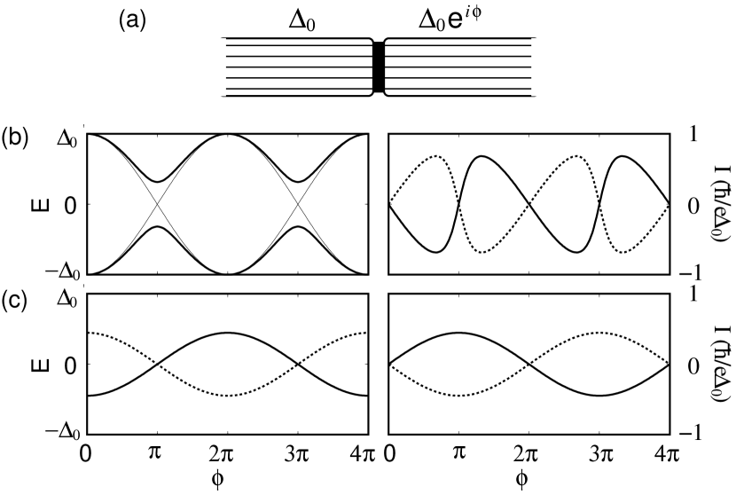
Figure 1: (a) Butt-to-butt Josephson junction between two Q1D $p_{x}$-wave superconductors. (b) The energies (left panel) and the currents (right panel) of the Andreev subgap states in the $s$-$s$ junction as functions of the phase difference $\phi$ for $D=1$ (thin lines) and $D=0.9$ (thick lines). (c) The same as (b) for the $p_{x}$-$p_{x}$ junction at $D=0.2$.

The energies (17) and (18) are plotted as functions of $\phi$ in the left panels (b) and (c) of Fig. 1. Without barrier ($D=1$), the spectra of the $s$-$s$ and $p_{x}$-$p_{x}$ junctions are the same and consist of two crossing curves $E=\mp\Delta_{0}\cos\phi/2$, shown by the thin lines in the left panel of Fig. 1(b). A nonzero barrier ($D<1$) affects the energies of the Andreev bound states in the $s$-$s$ and $p_{x}$-$p_{x}$ junctions in different ways. In the $s$-$s$ case, the two energy levels repel near $\phi=\pi$ and form two separated $2\pi$-periodic branches shown by the thick lines in the left panel of Fig. 1(b). This is well known for the $s$-$s$ junctions Zagoskin ; Furusaki99 . In contrast, in the $p_{x}$-$p_{x}$ case, the two energy levels continue to cross at $\phi=\pi$, and they detach from the continuum of states above $+\Delta_{0}$ and below $-\Delta_{0}$ at $\phi=0$ and $2\pi$, as shown in the left panel of Fig. 1(c). The absence of energy levels repulsion at $\phi=\pi$ indicates that there is no matrix element between these levels in the $p_{x}$-$p_{x}$ case, unlike in the $s$-$s$ case.

As shown in Sec. IV.1, the $45^{\circ}/45^{\circ}$ junction between two $d$-wave superconductors is mathematically equivalent to the $p_{x}$-$p_{x}$ junction. Eq. (18) was derived for the $45^{\circ}/45^{\circ}$ junction in Refs. Tanaka1 ; Riedel ; Barash .

III.2 dc Josephson effect in thermodynamic equilibrium

It is well known Zagoskin ; A-B that the current carried by a quasiparticle state $a$ is

$$I_{a}={2e\over\hbar}\,{\partial E_{a}\over\partial\phi}.$$ (19)

The two subgap states carry opposite currents, which are plotted vs. $\phi$ in the right panels (b) and (c) of Fig. 1 for the $s$-$s$ and $p_{x}$-$p_{x}$ junctions. In thermodynamic equilibrium, the total current is determined by the Fermi occupation numbers $f_{a}$ of the states at a temperature $T$:

$$I={2e\over\hbar}\sum_{a=\pm}{\partial E_{a}\over\partial\phi}\,f_{a}=-{2e\over\hbar}{\partial E_{0}\over\partial\phi}\tanh\left({E_{0}\over 2T}\right).$$ (20)

For the $s$-$s$ junction, substituting Eq. (17) into Eq. (20), we recover the Ambegaokar-Baratoff formula AB in the tunneling limit $D\ll 1$

$$I_{s}\approx D\sin\phi\,{e\Delta_{0}\over 2\hbar}\tanh\left({\Delta_{0}\over 2T}\right)=\sin\phi\,{\pi\Delta_{0}\over 2eR}\tanh\left({\Delta_{0}\over 2T}\right)$$ (21)

and the Kulik-Omelyanchuk formula KO in the transparent limit $D\to 1$

$$I_{s}\approx\sin\left({\phi\over 2}\right){e\Delta_{0}\over\hbar}\tanh\left({\Delta_{0}\cos(\phi/2)\over 2T}\right).$$ (22)

Taking into account that the total current is proportional to the number $N$ of conducting channels in the junction (e.g. the number of chains), we have replaced the transmission coefficient $D$ in Eq. (21) by the junction resistance $R=h/2Ne^{2}D$ in the normal state.

Substituting Eq. (18) into Eq. (20), we find the Josephson current in the $p_{x}$-$p_{x}$ junction in thermodynamic equilibrium:

$$I_{p}=\sqrt{D}\sin\left({\phi\over 2}\right){e\Delta_{0}\over\hbar}\tanh\left({\Delta_{0}\sqrt{D}\cos(\phi/2)\over 2T}\right)$$

$$=\sin\left({\phi\over 2}\right){\pi\Delta_{0}\over\sqrt{D}eR}\tanh\left({\Delta_{0}\sqrt{D}\cos(\phi/2)\over 2T}\right).$$ (23)

The temperature dependences of the critical currents for the $s$-$s$ and $p_{x}$-$p_{x}$ junctions are shown in Fig. 2. They are obtained from Eqs. (21) and (23) assuming the BCS temperature dependence for $\Delta_{0}$. In the vicinity of $T_{c}$, $I_{p}$ and $I_{s}$ have the same behavior. With the decrease of temperature, $I_{s}$ quickly saturates to a constant value, because, for $D\ll 1$, $E_{a}^{(s)}\approx\mp\Delta_{0}$ (17), thus, for $T\lesssim\Delta_{0}$, the upper subgap state is empty and the lower one is completely filled. In contrast, $I_{p}$ rapidly increases with decreasing temperature as $1/T$ and saturates to a value enhanced by the factor $2/\sqrt{D}$ relative to the Ambegaokar-Baratoff formula (17) at $T=0$. This is a consequence of two effects. As Eqs. (21) and (23) show, $I_{s}\propto D$ and $I_{p}\propto\sqrt{D}$, thus $I_{p}\gg I_{s}$ in the tunneling limit $D\ll 1$. At the same time, the energy splitting between the two subgap states in the $p_{x}$-$p_{x}$ junction is small compared to the gap: $E_{0}^{(p)}\propto\sqrt{D}\Delta_{0}\ll\Delta_{0}$. Thus, for $\sqrt{D}\Delta_{0}\lesssim T\lesssim\Delta_{0}$, the two subgap states are almost equally populated, so the critical current has the $1/T$ temperature dependence analogous to the Curie spin susceptibility.

Figure 2: Critical currents of the $s$-$s$ (dashed line) and $p_{x}$-$p_{x}$ (solid line) Josephson junctions as functions of temperature for $D=0.3$.

Eq. (23) was derived analytically for the $45^{\circ}/45^{\circ}$ junction between two $d$-wave superconductors in Refs. Riedel ; Tanaka2 , and a similar result was calculated numerically for the $p_{x}$-$p_{x}$ junction in Ref. Tanaka-pp ; Vaccarella . Notice that Eq. (23) gives the Josephson current $I_{p}(\phi)$ that is a $2\pi$-periodic functions of $\phi$, both for $T=0$ and $T\neq 0$. This is a consequence of the thermodynamic equilibrium assumption. At $T=0$, this assumption implies that the subgap state with the lower energy is occupied, and the one with the higher energy is empty. As one can see in Fig. 1, the lower energy is always a $2\pi$-periodic functions of $\phi$. The assumption of thermodynamic equilibrium was explicitly made in Ref. Riedel and was implicitly invoked in Refs. Tanaka2 ; Tanaka-pp ; Vaccarella by using the Matsubara diagram technique. In Ref. Arie , temperature dependence of the Josephson critical current was measured in the YBCO ramp-edge junctions with different crystal angles and was found to be qualitatively consistent with the upper curve in Fig. 2.

III.3 Dynamical fractional ac Josephson effect

The calculations of the previous section apply in the static case, where a given phase difference $\phi$ is maintained for an infinitely long time, so the occupation numbers of the subgap states have enough time to relax to thermodynamic equilibrium. Now let us consider the opposite, dynamical limit. Suppose a small voltage $eV\ll\Delta_{0}$ is applied to the junction, so the phase difference acquires dependence on time $t$: $\phi(t)=2eVt/\hbar$. In this case, the state of the system is determined dynamically starting from the initial conditions. Let us consider the $p_{x}$-$p_{x}$ junction at $T=0$ in the initial state $\phi=0$, where the two subgap states (18) with the energies $\pm E_{0}$ are, correspondingly, occupied and empty. If $\phi(t)$ changes sufficiently slowly (adiabatically), the occupation numbers of the subgap states do not change. In other words, the states shown by the solid and dotted lines in Fig. 1(c) remains, correspondingly, occupied and empty. The occupied state (18) produces the current (19):

$$I_{p}(t)={\sqrt{D}e\Delta_{0}\over\hbar}\sin\left({\phi(t)\over 2}\right)={\sqrt{D}e\Delta_{0}\over\hbar}\sin\left({eVt\over\hbar}\right).$$ (24)

The frequency of the ac current (24) is $eV/\hbar$, a half of the conventional Josephson frequency $2eV/\hbar$. The fractional frequency can be traced to the fact that the energies Eq. (18) and the corresponding wave functions have the period $4\pi$ in $\phi$, rather than conventional $2\pi$. Although at $\phi=2\pi$ the spectrum in the left panel of Fig. 1(c) is the same as at $\phi=0$, the occupation numbers are different: The lower state is empty and the upper state is occupied. Only at $\phi=4\pi$ the occupation numbers are the same as at $\phi=0$.

The $4\pi$ periodicity is the consequence of the energy levels crossing at $\phi=\pi$. (In contrast, in the $s$-wave case, the levels repel at $\phi=\pi$ in Fig. 1(b), thus the energy curves are $2\pi$-periodic.) As discussed at the end of Sec. III.1, there is no matrix element between the crossing energy levels at $\phi=\pi$. Thus, there are no transitions between them, so the occupation numbers of the solid and dotted curves in Fig. 1(c) are preserved. In order to show this more formally, we can write a general solution of the time-dependent BdG equation as a superposition of the two subgap states with the time-dependent $\phi(t)$: $\psi(t)=\sum_{a}C_{a}(t)\,\psi_{a}[\phi(t)]$. The matrix element of transitions between the states is proportional to $\dot{\phi}\langle\psi_{+}|\partial_{\phi}\psi_{-}\rangle=\dot{\phi}\langle\psi_{+}|\partial_{\phi}\hat{H}|\psi_{-}\rangle/(E_{-}-E_{+})$. We found that it is zero in the $p_{x}$-wave case, thus there are no transitions, and the initial occupation numbers of the subgap states at $\phi=0$ are preserved dynamically.

As one can see in Fig. 1(c), the system is not in the ground state when $\pi<\phi<3\pi$, because the upper energy level is occupied and the lower one is empty. In principle, the system might be able to relax to the ground state by emitting a phonon or a photon. At present time, we do not have an explicit estimate for such inelastic relaxation time, but we expect that it is quite long. (The other papers Riedel ; Tanaka2 ; Tanaka-pp ; Vaccarella that assume thermodynamic equilibrium for each value of the phase $\phi$ do not have an estimate of the relaxation time either.) To observe the predicted ac Josephson effect with the fractional frequency $eV/\hbar$, the period of Josephson oscillations should be set shorter than the inelastic relaxation time, but not too short, so that the time evolution of the BdG equation can be treated adiabatically. Controlled nonequilibrium population of the upper Andreev bound state was recently achieved experimentally in an $s$-wave Josephson junction in Ref. Baselmans .

Eq. (24) can be generalized to the case where initially the two subgap states are populated thermally at $\phi=0$, and these occupation numbers are preserved by dynamical evolution

$$I_{p}(t) = {2e\over\hbar}\sum_{a}{\partial E_{a}[\phi(t)]\over\partial\phi}\,f[E_{a}(\phi=0)]$$ (25)

$$= \sin\left({eVt\over\hbar}\right){\pi\Delta_{0}\over\sqrt{D}eR}\tanh\left({\Delta_{0}\sqrt{D}\over 2T}\right).$$ (26)

Notice that the periodicities of the dynamical equation (26) and the thermodynamic Eq. (23) are different. The latter equation assumes that the occupation numbers of the subgap states are in instantaneous thermal equilibrium for each $\phi$.

III.4 Tunneling Hamiltonian approach

In the infinite barrier limit $D\to 0$, the energies $\pm E_{0}^{(p)}$ of the two subgap states (18) degenerate to zero, i.e. they become midgap states. The wave functions (10) simplify as follows:

$$\psi_{\pm 0} = {\psi_{L0}(x)\mp\psi_{R0}(x)\over\sqrt{2}},$$ (27)

$$\psi_{L0} = \sqrt{2\kappa}\,\sin(k_{F}x)\,e^{\kappa x}\left(\begin{array}[]{c}1\\ i\end{array}\right)\theta(-x),$$ (30)

$$\psi_{R0} = \sqrt{2\kappa}\,\sin(k_{F}x)\,e^{-\kappa x}\left(\begin{array}[]{c}e^{i\phi/2}\\ -ie^{-i\phi/2}\end{array}\right)\theta(x).$$ (33)

Since at $D=0$ the Josephson junction consists of two semi-infinite uncoupled $p_{x}$-wave superconductors, $\psi_{L0}$ and $\psi_{R0}$ are the wave functions of the surface midgap states Ours1 belonging to the left and right superconductors. Let us examine the properties of the midgap states in more detail.

If $(u,v)$ is an eigenvector of Eq. (3) with an eigenvalue $E_{n}$, then $(-v^{*},u^{*})$ for $s$-wave and $(v^{*},u^{*})$ for $p$-wave are the eigenvectors with the energy $E_{\bar{n}}=-E_{n}$. It follows from these relations and Eq. (1) that $\hat{\gamma}_{\bar{n}\bar{\sigma}\bar{k}_{y}}=C\hat{\gamma}_{n\sigma k_{y}}^{\dagger}$ with $|C|=1$. Notice that in the $s$-wave case, because $(u,v)$ and $(-v^{*},u^{*})$ are orthogonal for any $u$ and $v$, the states $n$ and $\bar{n}$ are always different. However, in the $p$-wave case, the vectors $(u,v)$ and $(v^{*},u^{*})$ may be proportional, in which case they describe the same state with $E=0$. The states (30) and (33) indeed have this property:

$$v_{L0}=iu_{L0}^{*},\qquad v_{R0}=-iu_{R0}^{*}.$$ (34)

Substituting Eq. (34) into Eq. (1), we find the Bogoliubov operators of the left and right midgap states

$$\hat{\gamma}^{\dagger}_{L0\sigma k_{y}}=i\hat{\gamma}_{L0\bar{\sigma}\bar{k}_{y}},\quad\hat{\gamma}^{\dagger}_{R0\sigma k_{y}}=-i\hat{\gamma}_{R0\bar{\sigma}\bar{k}_{y}}.$$ (35)

Operators (35) correspond to the Majorana fermions discussed in Ref. Kitaev . In the presence of a midgap state, the sum over $n$ in Eq. (2) should be understood as $\sum_{n>0}+(1/2)\sum_{n=0}$, where we identify the second term as the projection ${\cal P}\hat{c}$ of the electron operator onto the midgap state. Using Eqs. (34), (35), and (2), we find

$${\cal P}\hat{c}_{\sigma k_{y}}(x)=u_{0}(x)\hat{\gamma}_{0\sigma k_{y}}=v_{0}^{*}(x)\hat{\gamma}_{0\bar{\sigma}\bar{k}_{y}}^{\dagger}.$$ (36)

Let us consider two semi-infinite $p_{x}$-wave superconductors on a 1D lattice with the spacing $l$, one occupying $x\leq\bar{l}=-l$ and another $x\geq l$. They are coupled by the tunneling matrix element $\tau$ between the sites $\bar{l}$ and $l$:

$$\hat{H}_{\tau}=\tau\sum_{\sigma k_{y}}[\hat{c}^{\dagger}_{L\sigma k_{y}}(\bar{l})\,\hat{c}_{R\sigma k_{y}}(l)+\hat{c}^{\dagger}_{R\sigma k_{y}}(l)\,\hat{c}_{L\sigma k_{y}}(\bar{l})].$$ (37)

In the absence of coupling ($\tau=0$), the subgap wave functions of each superconductor are given by Eqs. (30) and (33). Using Eqs. (36), (34), (30), and (33), the tunneling Hamiltonian projected onto the basis of midgap states is

$${\cal P}\hat{H}_{\tau}=\tau\,[u_{L0}^{*}(\bar{l})u_{R0}(l)+{\rm c.c.}]\,(\hat{\gamma}_{L0\uparrow}^{\dagger}\hat{\gamma}_{R0\uparrow}+{\rm H.c.})$$

$$=\Delta_{0}\sqrt{D}\,\cos(\phi/2)\,(\hat{\gamma}_{L0\uparrow}^{\dagger}\hat{\gamma}_{R0\uparrow}+\hat{\gamma}_{R0\uparrow}^{\dagger}\hat{\gamma}_{L0\uparrow}),$$ (38)

where $\sqrt{D}=4\tau\sin^{2}k_{F}l/\hbar v_{F}$ is the transmission amplitude, and we omitted summation over the diagonal index $k_{y}$. Notice that Eq. (38) is $4\pi$-periodic in $\phi$ Kitaev .

Hamiltonian (38) operates between the two degenerate states of the system related by annihilation of the Bogoliubov quasiparticle in the right midgap state and its creation in the left midgap state. In this basis, Hamiltonian (38) can be written as a $2\times 2$ matrix

$${\cal P}\hat{H}_{\tau}=\Delta_{0}\sqrt{D}\cos(\phi/2)\left(\begin{array}[]{cc}0&1\\ 1&0\end{array}\right).$$ (39)

The eigenvectors of Hamiltonian (39) are $(1,\mp 1)$, i.e. the antisymmetric and symmetric combinations of the right and left midgap states given in Eq. (27). Their eigenenergies are $E_{\pm}(\phi)=\mp\Delta_{0}\sqrt{D}\cos(\phi/2)$, in agreement with Eq. (18). The tunneling current operator is obtained by differentiating Eqs. (38) or (39) with respect to $\phi$. Because $\phi$ appears only in the prefactor, the operator structures of the current operator and the Hamiltonian are the same, so they are diagonal in the same basis. Thus, the energy eigenstates are simultaneously the eigenstates of the current operator with the eigenvalues

$$I_{\pm}=\pm{\sqrt{D}e\Delta_{0}\over\hbar}\sin\left({\phi\over 2}\right),$$ (40)

in agreement with Eq. (24). The same basis $(1,\mp 1)$ diagonalizes Hamiltonian (39) even when a voltage $V$ is applied and the phase $\phi$ is time-dependent. Then the initially populated eigenstate with the lower energy produces the current $I_{p}=\sqrt{D}(e\Delta_{0}/\hbar)\sin(eVt/\hbar)$ with the fractional Josephson frequency $eV/\hbar$, in agreement with Eq. (24).

III.5 Josephson current carried by single electrons, rather than Cooper pairs

In the tunneling limit, the transmission coefficient $D$ is proportional to the square of the electron tunneling amplitude $\tau$: $D\propto\tau^{2}$. Eqs. (24) and (40) show that the Josephson current in the $p_{x}$-$p_{x}$ junction is proportional to the first power of the electron tunneling amplitude $\tau$. This is in contrast to the $s$-$s$ junction, where the Josephson current (21) is proportional to $\tau^{2}$. This difference results in the big ratio $I_{p}/I_{s}=2/\sqrt{D}$ between the critical currents at $T=0$ in the $p_{x}$- and $s$-wave cases, as shown in Fig. 2 and discussed in Sec. III.2. The reason for the different powers of $\tau$ is the following. In the $p_{x}$-wave case, the transfer of just one electron between the degenerate left and right midgap states is a real (nonvirtual) process. Thus, the eigenenergies are determined from the secular equation (39) already in the first order of $\tau$. In the $s$-wave case, there are no midgap states, so the transferred electron is taken from below the gap and placed above the gap, at the energy cost $2\Delta_{0}$. Thus, the transfer of a single electron is a virtual (not real) process. It must be followed by the transfer of another electron, so that the pair of electrons is absorbed into the condensate. This gives the current proportional to $\tau^{2}$.

This picture implies that the Josephson supercurrent across the interface is carried by single electrons in the $p_{x}$-$p_{x}$ junction and by Cooper pairs in the $s$-$s$ junction. Because the single-electron charge $e$ is a half of the Cooper-pair charge $2e$, the frequency of the ac Josephson effect in the $p_{x}$-$p_{x}$ junction is $eV/\hbar$, a half of the conventional Josephson frequency $2eV/\hbar$ for the $s$-$s$ junction. These conclusions also apply to a junction between two cuprate $d$-wave superconductors in such orientation that both sides of the junction have surface midgap states, e.g. to the $45^{\circ}/45^{\circ}$ junction (see Sec. IV.1).

In both the $p_{x}$-$p_{x}$ and $s$-$s$ junctions, electrons transferred across the interface are taken away into the bulk by the supercurrent of Cooper pairs. In the case of the $p_{x}$-$p_{x}$ junction, a single transferred electron occupies a midgap state until another electron gets transferred. Then the pair of electrons becomes absorbed into the bulk condensate, the midgap state returns to the original configuration, and the cycle repeats. In the case of the $s$-$s$ junction, two electrons are simultaneously transferred across the interface and become absorbed into the condensate. Clearly, electric charge is transferred across the interface by single electrons at the rate proportional to $\tau$ in the first case and by Cooper pairs at the rate proportional to $\tau^{2}$ in the second case, but the bulk supercurrent is carried by the Cooper pairs in both cases.

III.6 Josephson effect between triplet superconductors with nonparallel $\bm{n}$-vectors

In this section, we consider the Josephson effect between two $p_{x}$-wave superconductors with nonparallel spin-polarization vectors $\bm{n}$ forming an angle $\theta$. This problem was studied in Ref. Vaccarella using a tunneling Hamiltonian approach. Here we analyze the problem using the BdG formulation. There are experimental indications that the spin-polarization vector $\bm{n}$ is parallel to the crystal axis $\bm{c}$ in the $\rm(TMTSF)_{2}X$ compounds Chaikin ; Lebed . Then the considered junction can be realized in the geometry shown in Fig. 1(a) where the $\bm{c}$ axes of the two superconductors are rotated relative to each other by the angle $\theta$ around the common $\bm{a}$ axis along the chains.

Let us select the spin quantization axis $z$ perpendicular to both vectors $\bm{n}$, and the $x$ axis in the spin space parallel to the vector $\bm{n}$ of the left superconductor. Then the vector $\bm{n}$ of the right superconductor lies in the $(x,y)$ plane at the angle $\theta$ to the $x$ axes: $\bm{n}=(\cos\theta,\sin\theta,0)$. In this representation, the superconducting pairing takes place between electrons with parallel spins:

$$\langle\hat{c}_{\sigma}(\bm{k})\hat{c}_{\sigma^{\prime}}(-\bm{k})\rangle \propto i\hat{\sigma}^{(y)}\,(\hat{\sigma}^{(x)}n_{x}+\hat{\sigma}^{(y)}n_{y})\,\Delta(\bm{k})$$ (43)

$$= \left(\begin{array}[]{cc}e^{i\theta}&0\\ 0&-e^{-i\theta}\end{array}\right)\Delta(\bm{k}).$$

Then, the Josephson effect can be considered separately for the spin up and down sectors having the phase differences $\phi\pm\theta$, correspondingly. Using Eq. (18) for the $p_{x}$-$p_{x}$ junction, we find the energies of the Andreev bound states for each spin sector

$$E_{a,\uparrow} = -a\Delta_{0}\sqrt{D}\cos\left({\phi+\theta\over 2}\right),$$ (44)

$$E_{a,\downarrow} = -a\Delta_{0}\sqrt{D}\cos\left({\phi-\theta\over 2}\right).$$ (45)

The total Josephson current is obtained by adding the currents carried by the two spin sectors double . For simplicity, below we consider only the case of zero temperature. In the dynamical limit, assuming that the states (44) and (45) with $a=+$ are occupied initially and the occupation numbers are preserved dynamically and using Eq. (24), we find a $4\pi$-periodic current:

$$I(t) = {\sqrt{D}e\Delta_{0}\over 2\hbar}\left[\sin\left({\phi+\theta\over 2}\right)+\sin\left({\phi-\theta\over 2}\right)\right]$$ (46)

$$= {\sqrt{D}e\Delta_{0}\over\hbar}\,\sin\left({\phi(t)\over 2}\right)\,\cos\left({\theta\over 2}\right).$$

In the static thermodynamic limit, using Eq. (23) at $T=0$, we find the dc Josephson current:

$$I = {\sqrt{D}e\Delta_{0}\over 2\hbar}\left\{\sin\left({\phi+\theta\over 2}\right)\,{\rm sgn}\left[\cos\left({\phi+\theta\over 2}\right)\right]\right.$$ (47)

$$+\left.\sin\left({\phi-\theta\over 2}\right)\,{\rm sgn}\left[\cos\left({\phi-\theta\over 2}\right)\right]\right\}.$$

For completeness, let us also consider the Josephson effect between two $p_{y}$-wave or two $p_{z}$-wave superconductors, where the $y$ and $z$ axes are parallel to the junction plane. In these junctions, midgap states are absent in the $D\to 0$ limit, thus the current-phase relation is conventional $I=I_{c}\sin\phi$. For nonparallel vectors $\bm{n}$, the total Josephson current is the sum of the spin up and down sectors:

$$I = {I_{c}\over 2}\,[\sin(\phi+\theta)+\sin(\phi-\theta)]$$ (48)

$$= I_{c}\cos\theta\sin\phi=I_{c}(\bm{n}_{L}\cdot\bm{n}_{R})\sin\phi.$$

Eq. (48) is consistent with Ref. Vaccarella . In the case where the two vectors $\bm{n}$ are perpendicular ($\theta=\pi/2$), the Josephson current (48) for the superconductors without midgap states vanishes, but, according to Eqs. (46) and (47), it is not zero if the midgap states are present.

III.7 $s$-$p_{x}$ junction between singlet and triplet superconductors

In this section, we consider a junction between a singlet $s$-wave and a triplet $p_{x}$-wave superconductors. The junction geometry is the same as in Fig. 1(a), where one of the superconductors is taken to be a conventional $s$-wave superconductor and another one a Q1D triplet $p_{x}$-wave superconductor, such as $\rm(TMTSF)_{2}X$.

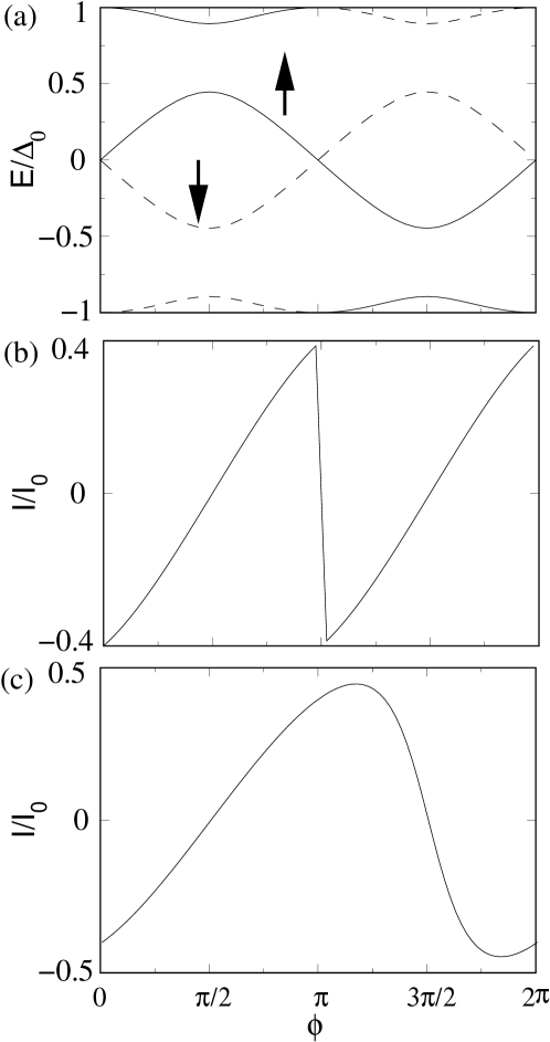
Figure 3: The subgap energy levels and the Josephson currents in the $s$-$p_{x}$ junction. Here $D=0.8$ and $I_{0}=e\Delta_{0}/2\hbar$. (a) The energies (49) of the Andreev bound states. The solid and dashed lines correspond to $\sigma=\uparrow$ and $\sigma=\downarrow$. (b) The Josephson current in the static thermodynamic limit, where the states with $E<0$ are occupied. (c) The Josephson current in the dynamical limit, where the central branch with $\sigma=\downarrow$ and the lower branches touching $-\Delta_{0}$ are occupied.

We choose the spin quantization axis $z$ along the polarization vector $\bm{n}$ of the triplet superconductor, so the spin projection $\sigma$ on the $z$ axis is a good quantum number. In both triplet and singlet superconductors, the Cooper pairing takes place between electrons with opposite spins. However, the pairing potential has the same sign for $\sigma$ and $\bar{\sigma}$ in the triplet superconductor and the opposite signs in the singlet superconductor. Thus, the phase difference across the Josephson junction is $\phi$ for quasiparticles with $\sigma=\uparrow$ and $\phi+\pi$ for $\sigma=\downarrow$. The energies of the Andreev bound states can be found for each $\sigma$ from Eq. (16) together with Eq. (11), where we should use the upper line of Eq. (14) for the left superconductor and the lower line for the right superconductor. To simplify calculations, we consider the case where the magnitudes of the gaps are equal for the $s$- and $p_{x}$-wave superconductors: $|\Delta_{L}|=|\Delta_{R}|=\Delta_{0}$. The energies of the Andreev bound states are

$$E_{a,\sigma}=\sigma\,{\rm sgn}(\sin\phi)\Delta_{0}\sqrt{1+a\sqrt{1-D^{2}\sin^{2}\phi}\over 2}.$$ (49)

For each value of the spin index $\sigma=\pm$, Eq. (49) gives two Andreev states labeled by the index $a=\pm$. In the tunneling limit $D\ll 1$, we have

$$E_{+,\sigma} \approx \sigma\,{\rm sgn}(\sin\phi)\,\Delta_{0}\left(1-\frac{1}{8}\,D^{2}\sin^{2}\phi\right),$$ (50)

$$E_{-,\sigma} \approx \frac{1}{2}\,\sigma\Delta_{0}D\sin\phi.$$ (51)

The energies (49) are plotted in Fig. 3(a) vs. $\phi$ by the solid lines for $\sigma=\uparrow$ and by the dashed lines for $\sigma=\downarrow$. We observe that the branches (50) with $a=+$ touch the gap boundaries $\pm\Delta_{0}$ at $\phi=0$ and $\pi$, whereas the branches (51) with $a=-$ stay in the center of the gap.

In the limit $D\ll 1$, the central branches with $a=-$ dominate the energy dependence on $\phi$, and energy minima are achieved at $\phi=\pi/2$ or $3\pi/2$. Notice that if the system selects the energy minimum at $\phi=\pi/2$, then the spin down states, shown by the dashed lines in Fig. 3(a), are populated, and the spin up states are empty, so the junction accumulates the spin $-\hbar/2$ per conducting channel double . If the system selects the energy minimum at $\phi=3\pi/2$, then the junction accumulates the spin $\hbar/2$ per conducting channel.

In the limit $D\ll 1$, we can neglect the energies (50) and obtain the Josephson current by differentiating the energies (51) with respect to $\phi$ using Eq. (19) double . In the dynamical limit, the occupation numbers of the Andreev states (51) are preserved, and the Josephson current has the $2\pi$-periodicity, as shown in Fig. 3(c):

$$I(t)\approx-{e\over 2\hbar}\Delta_{0}D\cos\phi(t).$$ (52)

In the static thermodynamic limit, the system occupies the branch of the minimal energy for each $\phi$, and the Josephson current is $\pi$-periodic, as shown in Fig. 3(b):

$$I(\phi)\approx-{e\over 2\hbar}\Delta_{0}D\,{\rm sgn}(\sin\phi)\,\cos\phi.$$ (53)

The thermodynamic assumption implies that the spin accumulation at the $s$-$p_{x}$ junction changes sign when the phase $\phi$ crosses $\pi$.

Figure 4: A Q1D $p_{x}$-wave superconductor closed in a loop by an $s$-wave superconductor. No current is circulating in the loop in equilibrium. However, there is accumulation of spins up in one $s$-$p_{x}$ junction and spins down in another junction. The sketch at the top illustrates the Fermi surface of a Q1D metal with the opposite signs of the superconducting $p_{x}$-wave pairing potential on the two sheets of the Fermi surface.

Now let us consider the circuit shown in Fig. 4, where a $p_{x}$-wave superconductor has Josephson junctions at both ends with an $s$-wave superconductor closed in a loop. Because the sign of the $p_{x}$-wave pairing potential is opposite for the $+k_{F}$ and $-k_{F}$ sheets of the Fermi surface, the two junctions have the relative phase shift $\pi$. Naively, one might expect a spontaneous current in this circuit by analogy with the corner SQUID in the cuprates vanHarlingen . However, the system shown in Fig. 4 can accommodate the phase shift $\pi$ by selecting the energy minimum at $\phi=\pi/2$ for one junction and the energy minimum at $\phi=3\pi/2$ for another junction. Then, no current circulates in the loop. However, one junction accumulates spins up and another junction spins down, which might be possible to detect experimentally.

The results of the this section clearly show that a Josephson current is possible between singlet and triplet superconductors, in agreement with the earlier findings by Yip Yip . Recently, the Josephson current was calculated for the $s$-$p_{x}$ junction in Ref. Asano , but spin accumulation at the junction was not recognized in this paper. The $s$-$p_{x}$ junction considered in this section is mathematically equivalent to the $0^{\circ}/45^{\circ}$ $d$-$d$ junction and the $45^{\circ}$ junction between an $s$-wave and a $d$-wave superconductors (see Sec. IV.1). Eq. (49) was obtained for that case in Refs. Riedel ; Barash ; Tanaka2 . However, there is no spin accumulation in junctions between singlet $s$- and $d$-wave superconductors, unlike in the $s$-$p_{x}$ junction.

IV Junctions between quasi-two-dimensional superconductors

In this section, we study junctions between quasi-two-dimensional (Q2D) superconductors such as nonchiral $d$-wave cuprates and chiral $p_{x}\pm ip_{y}$-wave ruthenates. For simplicity, we use an isotropic electron energy dispersion law $\varepsilon=\hbar^{2}(k_{x}^{2}+k_{y}^{2})/2m-\mu$ in the $(x,y)$ plane. As before, we select the coordinate $x$ perpendicular to the junction line and assume that the electron momentum component $k_{y}$ parallel to the junction line is a conserved good quantum number. Then, the 2D problem separates into a set of 1D solutions (10) in the $x$ direction labeled by the index $k_{y}$. The Fermi momentum $k_{F}$ and velocity $v_{F}$ are replaced by their $x$-components $k_{Fx}=\sqrt{k_{F}^{2}-k_{y}^{2}}$ and $v_{Fx}=\hbar k_{Fx}/m$. The transmission coefficient of the barrier (9) becomes $k_{y}$-dependent

$$Z(k_{y})=Z_{0}{k_{F}\over\sqrt{k_{F}^{2}-k_{y}^{2}}},\quad D(k_{y})={4\over Z^{2}(k_{y})+4},$$ (54)

where $Z_{0}=\sqrt{2mU_{0}}/\hbar k_{F}$. The total Josephson current is given by a sum over all occupied subgap states labeled by $k_{y}$.

IV.1 Josephson junctions between $d$-wave superconductors

For the cuprates, let us consider a junction parallel to the $[1,\bar{1}]$ crystal direction in the $(\bm{a},\bm{b})$ plane and select the $x$ axis along the diagonal $[1,1]$, as shown in Fig. 5(a). In these coordinates, the $d$-wave pairing potential is

$$\hat{\Delta}_{\sigma k_{y}}(x,\hat{k}_{x})=\sigma 2\Delta_{\beta}\,k_{y}\hat{k}_{x}/k_{F}^{2},$$ (55)

where the same notation as in Eq. (6) is used. Direct comparison of Eqs. (55) and (6) demonstrates that the $d$-wave superconductor with the $45^{\circ}$ junction maps to the $p_{x}$-wave superconductor by the substitution $\Delta_{0}\to\sigma 2\Delta_{0}k_{y}/k_{F}$. Thus, the results obtained in Sec. III for the $p_{x}$-$p_{x}$ junction apply to the $45^{\circ}/45^{\circ}$ junction between two $d$-wave superconductors with the appropriate integration over $k_{y}$. The energies of the subgap Andreev states are given by Eq. (18) with the $k_{y}$-dependent parameters $\Delta_{0}$ and $D$, and the energies and the wave functions are $4\pi$-periodic functions of $\phi$. Thus, the ac Josephson current in the dynamical limit is $4\pi$-periodic and has the fractional frequency $eV/\hbar$, as in Eqs. (24), (26), and (40). The energies (18) of the subgap states Tanaka1 ; Riedel and the dc Josephson current (23) in the thermodynamic limit Riedel ; Tanaka2 were calculated for the $45^{\circ}/45^{\circ}$ $d$-$d$ junction before. However, these papers did not recognize the fractional, $4\pi$-periodic character of the Josephson effect in the dynamical limit.

Figure 5: Schematic drawing of the $45^{\circ}/45^{\circ}$ junction (panel a) and $0^{\circ}/0^{\circ}$ junction (panel b) between two $d$-wave superconductors. The thick line represents the junctions line. The circles illustrate the Fermi surfaces, where positive and negative pairing potentials $\Delta$ are shown by the solid and dotted lines. The points A, B, C, and D in the momentum space are connected by transmission and reflection from the barrier.

On the other hand, if the junction is parallel to the $[0,1]$ crystal direction, as shown in Fig. 5(b), then $\hat{\Delta}_{\sigma k_{y}}(x,\hat{k}_{x})=\sigma\Delta_{\beta}\,(\hat{k}_{x}^{2}-k_{y}^{2})/k_{F}^{2}$. This pairing potential is an even function of $\hat{k}_{x}$, thus it is analogous to the $s$-wave pairing potential in Eq. (6). Then, the $0^{\circ}/0^{\circ}$ junction between two $d$-wave superconductors is analogous to the $s$-$s$ junction. It should exhibit the conventional $2\pi$-periodic Josephson effect with the frequency $2eV/\hbar$.

For a generic orientation of the junction line, the $d$-wave pairing potential is $p_{x}$-like for some momenta $k_{y}$ and $s$-like for other $k_{y}$. Thus, the total Josephson current is a sum of the unconventional and conventional terms:

$$I=C_{0}\sin(\phi/2)+C_{1}\sin(\phi)+\ldots~{},$$ (56)

where $C_{0}$ and $C_{1}$ are some coefficients. We expect that both terms in Eq. (56) are present for any real junction between $d$-wave superconductors because of imperfections in junction orientation. However, the ratio $C_{0}/C_{1}$ should be maximal for the junction shown in Fig. 5(a) and minimal for the junction shown in Fig. 5(b). In general, whenever the superconductors on both sides of the junction have surface midgap states, we expect to observe the $4\pi$-periodic fractional ac Josephson effect. In principle, the effect may be spoiled by the gapless quasiparticles that exist near the gap nodes in a $d$-wave superconductor. However, they would affect only a small portion of the Fermi surface near the nodes, and the $4\pi$-periodic Josephson effect should survive on the other parts of the Fermi surface, where the gap is big.

The $45^{\circ}/45^{\circ}$ junction shown in Fig. 5(a) should not be confused with the $0^{\circ}/45^{\circ}$ $d$-$d$ junction Wendin-ac or the $45^{\circ}$ $s$-$d$ junction Tanaka-sd ; Zagoskin-sd , much discussed in literature. None of the papers Tanaka-sd ; Zagoskin-sd ; Wendin-ac treated the problem correctly, because they did not take into account the Andreev bound states in the junction properly. The correct energy spectrum of the Andreev bound states was obtained in Refs. Tanaka1 ; Riedel ; Barash . In the $0^{\circ}/45^{\circ}$ $d$-$d$ and $45^{\circ}$ $s$-$d$ junctions, only one superconductor has midgap states, thus these junctions are mathematically analogous to the $s$-$p_{x}$ junction considered in Sec. III.7. The spectrum of the Andreev bound states is given by Eq. (49) without the factor $\sigma$, because both superconductors are singlet. The energy levels are plotted vs. $\phi$ in Fig. 3(a), where the solid and dashed lines represent not spin, but positive and negative momenta $k_{y}$. The junction has two energy minima at $\phi=\pi/2$ or $3\pi/2$, where the states with only negative or positive momenta $k_{y}$ are filled, thus there are persistent currents along the junction line Huck ; Amin . (On the other hand, there is no spin accumulation, unlike in the $s$-$p_{x}$ junction discussed in Sec. III.7.) In the thermodynamic limit, the current-phase relation shown in Fig. 3(b) is $\pi$-periodic; however, it requires reversing the currents along the junction line when $\phi$ passes through 0 or $\pi$. In the dynamical limit, the current-phase relation shown in Fig. 3(c) is $2\pi$-periodic. The first two harmonics $I=C_{1}\sin(\phi)+C_{2}\sin(2\phi)$ have been recently observed experimentally in the $0^{\circ}/45^{\circ}$ $d$-$d$ junction Lindstrom .

IV.2 Josephson junctions with chiral superconductors

In this section, we study junctions between the chiral $p_{x}\pm ip_{y}$-wave superconductors $\rm Sr_{2}RuO_{4}$, where the pairing potential is assumed to be $\Delta({\bf k})=\Delta_{0}(k_{x}\pm ik_{y})/k_{F}$ Maeno , and the two signs correspond to opposite chiralities. We assume a uniform orientation of the spin-polarization vector $\bm{n}$ across the junction. This problem was investigated in Ref. Barash-chiral using the Eilenberger equation for Green’s functions. It was found that the chiral subgap states at the junctions enhance the low-temperature critical Josephson current in symmetric junctions. Here we use the BdG equation to obtain the spectrum of the Andreev bound states. As before, we assume that the momentum component $k_{y}$ parallel to the junction is conserved. Thus, the problem separates into a set of 1D solutions in the $x$ direction perpendicular to the junction plane, and we can use the method of Sec. III.1.

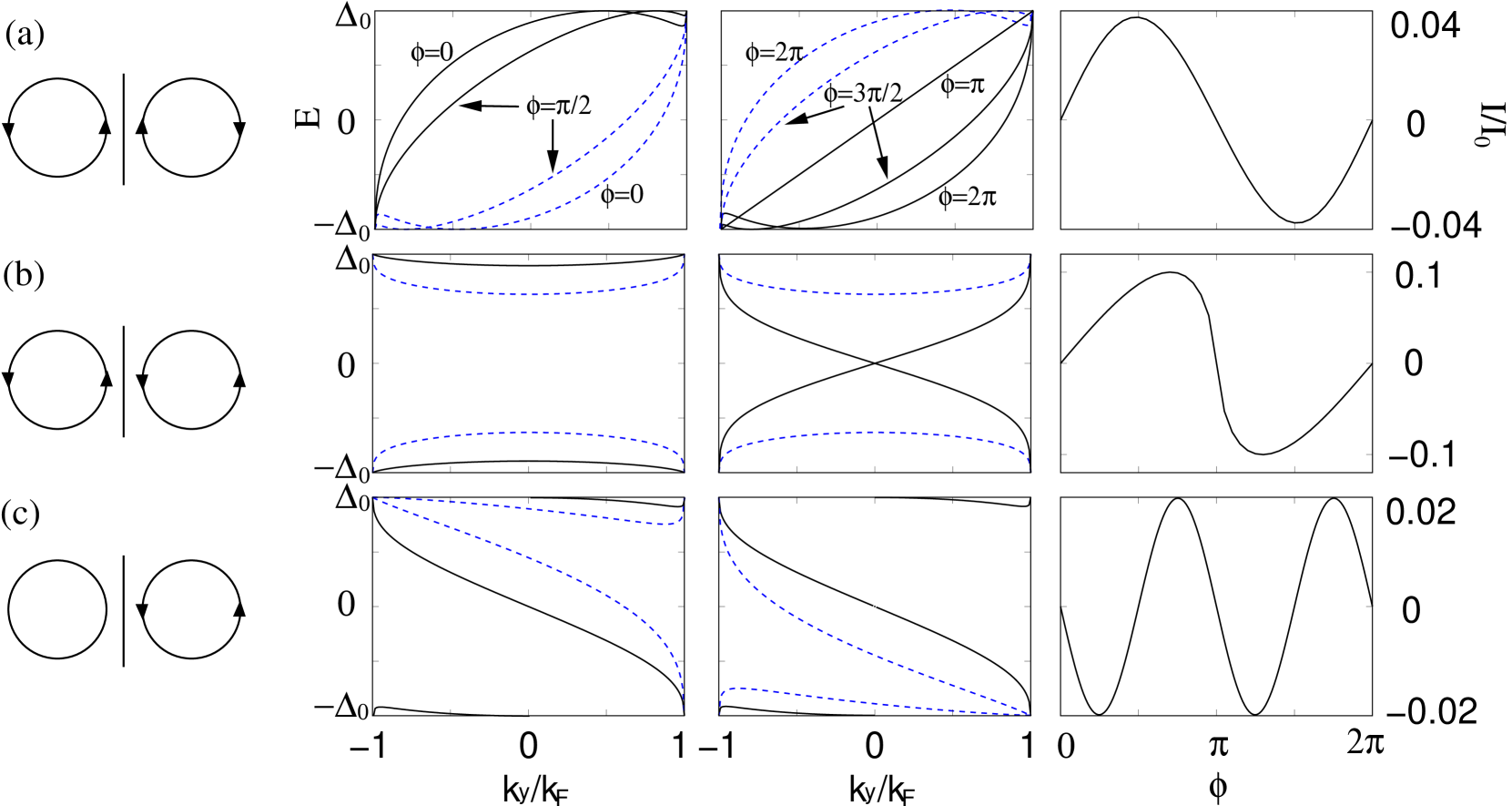
Figure 6: The subgap energy spectra and the Josephson currents in the junctions with chiral $p_{x}\pm ip_{y}$-wave superconductors, calculated for $Z_{0}=1$. (a) Junction between two $p$-wave superconductors with opposite chiralities. (b) Junction between two $p$-wave superconductors with the same chirality. (c) Junction between $s$-wave and chiral $p$-wave superconductors. In the second and third columns of row (a), the solid and dashed lines show the $a=\pm$ branches of Eq. (57) for different values of $\phi$. In rows (b) and (c), the energies (58) and (IV.2) are shown by the solid and dashed lines for $\phi=0$ and $\pi/2$ in the second column and for $\phi=\pi$ and $3\pi/2$ in the third column. The energies of quasiparticles with $\sigma=\downarrow$ are the same as with $\sigma=\uparrow$ for rows (a) and (b), and they can be obtained by the shift $\phi\to\phi+\pi$ for row (c). The fourth column shows the Josephson current in the static thermodynamic limit, normalized by $I_{0}=e\Delta_{0}L_{y}k_{F}/2\pi\hbar$, where $L_{y}$ is the length of the junction.

First we consider a junction between two superconductors with opposite chiralities, as illustrated in the first column of Fig. 6(a). In this case, $\Delta_{L}=\Delta_{0}(k_{x}+ik_{y})/k_{F}$ and $\Delta_{R}=e^{i\phi}\Delta_{0}(k_{x}-ik_{y})/k_{F}$. When the barrier is not transparent ($D=0$), each superconductor has chiral Andreev surface states with the same energy dispersion $E(k_{y})=k_{y}\Delta_{0}/k_{F}$ Honerkamp98 . The electron tunneling amplitude $\tau\propto\sqrt{D}$ produces a matrix element mixing the two states in the first-order degenerate perturbation theory. Thus, the two energy spectra repel with the splitting proportional to $\sqrt{D}$. From Eq. (16), we find the following subgap energies:

$$E={\Delta_{0}\over k_{F}}\left(k_{y}\sqrt{1-D\cos^{2}{\phi\over 2}}\pm\sqrt{k_{F}^{2}-k_{y}^{2}}\sqrt{D}\cos{\phi\over 2}\right).$$ (57)

The energy levels splitting oscillates with the period $4\pi$ as a function of $\phi$: $\delta E=(\Delta_{0}/k_{F})\sqrt{k_{F}^{2}-k_{y}^{2}}\sqrt{D}\cos\phi/2$. The splitting depends on $k_{y}$ through the square-root prefactor and through the dependence of $D$ on $k_{y}$ in Eq. (54), and vanishes at $k_{y}=\pm k_{F}$. The energy dispersion (57) is plotted vs. $k_{y}$ in the second and third columns of Fig. 6(a) for several values of $\phi$. The spectrum of excitations is gapless because of the chiral dispersion in $k_{y}$. Thus, it is reasonable to assume that the occupation numbers of the subgap states are in instantaneous thermodynamic equilibrium for any phase $\phi$. Then, the Josephson current is a $2\pi$-periodic function of $\phi$, as illustrated at zero temperature in the fourth column of Fig. 6(a), even though the energy levels (57) are $4\pi$-periodic functions of $\phi$.

Now let us consider the case of two superconductors with opposite chiralities, as illustrated in the first column of Fig. 6(b). When the two superconductors are disconnected ($D=0$), their chiral Andreev surface states have opposite dispersions $E=\pm k_{y}\Delta_{0}/k_{F}$, thus they are nondegenerate. The electron tunneling amplitude $\tau\propto\sqrt{D}$ repels the energy levels around the intersection point $k_{y}=0$. From Eq. (16), we find the following subgap energies:

$$E=\pm{\Delta_{0}\over k_{F}}\sqrt{(1-D)k_{y}^{2}+Dk_{F}^{2}\cos^{2}{\phi\over 2}}.$$ (58)

The energy dispersion (58) is plotted vs. $k_{y}$ in the second and third columns of Fig. 6(b) for several values of $\phi$. The energy splitting around $k_{y}=0$ is a $2\pi$-periodic function of $\phi$ and vanishes at $\phi=\pi$. The Josephson current is a $2\pi$-periodic function of $\phi$, as illustrated at zero temperature in the fourth column of Fig. 6(b).

Now let us consider a junction between an $s$-wave and a $p_{x}+ip_{y}$-wave superconductors shown in the first column of Fig. 6(c). The Josephson current was calculated in this case in Ref. Asano using the method of Green’s functions. However, the energies of the Andreev bound states were not written explicitly. The subgap states in this junction are obtained by solving Eq. (16) in the manner similar to the 1D $s$-$p_{x}$ junction. For simplicity, we assume that the magnitudes of the pairing potentials in both superconductors are the same: $|\Delta_{L}|=|\Delta_{R}|=\Delta_{0}$. The square of the subgap energies is given by the following expression

$$E_{a,\sigma}^{2} = {\Delta_{0}^{2}\over 2}\bigg{(}1+R\tilde{k}_{y}^{2}-\sigma D\tilde{k}_{y}\sin\phi$$

$$\left.{}+a\sqrt{1-\tilde{k}_{y}^{2}}\sqrt{1-(R\tilde{k}_{y}-\sigma D\sin\phi)^{2}}\right),$$

where $R=1-D$ is the reflection coefficient, and $\tilde{k}_{y}=k_{y}/k_{F}$. The signs of the energies are

$${\rm sgn}E_{a,\sigma} = {\rm sgn}\bigg{(}-R\tilde{k}_{y}+\sigma D\sin\phi$$

$$\left.{}+a\tilde{k}_{y}\sqrt{1-(R\tilde{k}_{y}-\sigma D\sin\phi)^{2}\over 1-\tilde{k}_{y}^{2}}\right).$$

For a given $\sigma$, there are two branches of energies labeled by the index $a=\pm$. The energy dispersions $E_{\pm,\uparrow}(k_{y})$ are shown in the second and third columns of Fig. 6(c) for several phases $\phi$. In the limit of impenetrable barrier $D\to 0$, the energy branch with $a=+$ approaches to the gap edges $|E_{+}|\to\Delta_{0}$, whereas the branch with $a=-$ approaches to the energy dispersion $E_{-}\to-k_{y}\Delta_{0}/k_{F}$ of the chiral surface states in the $p_{x}+ip_{y}$-wave superconductor Honerkamp98 .

The energy $E_{a,\sigma}(k_{y})$ for a given $\sigma$ is a $2\pi$-periodic function of $\phi$. The energy $E_{a,\bar{\sigma}}(k_{y})$ is obtained from $E_{a,\sigma}(k_{y})$ by the shift $\phi\to\phi+\pi$, as discussed in Sec. III.7. Thus, the Josephson current (20) in the static thermodynamic limit, obtained by summation over $\sigma$ and $k_{y}$, is a $\pi$-periodic function of $\phi$, as shown in the fourth column of Fig. 6(c), in agreement with Ref. Asano . Similarly to the $s$-$p_{x}$ junction considered in Sec. III.7, the $s$-($p_{x}+ip_{y}$) junction has two equal energy minima Asano at $\phi=\pi/2$ and $3\pi/2$ accompanied by accumulation of the down spin for $\phi=\pi/2$ and the up spin for $\phi=3\pi/2$.

V Experimental observation of the fractional ac Josephson effect

Conceptually, the setup for experimental observation of the fractional ac Josephson effect is straightforward. One should apply a dc voltage $V$ to the junction and measure frequency spectrum of microwave radiation from the junction, expecting to detect a peak at the fractional frequency $eV/\hbar$. Higher harmonics, such as $2eV/\hbar$, may also be present because of Eq. (56) and circuit nonlinearities, but an observation of the 1/2 subharmonic of the conventional Josephson frequency $2eV/\hbar$ would be the signature of the effect.

Josephson radiation at the conventional frequency $2eV/\hbar$ was first observed experimentally almost 40 years ago in Kharkov Yanson1 ; Yanson2 , followed by further work Langenberg ; Yanson3 . In Ref. Yanson2 , the spectrum of microwave radiation from tin junctions was measured, and a sharp peak at the frequency $2eV/\hbar$ was found. Without any attempt to match impedances of the junction and waveguide, Dmitrenko and Yanson Yanson2 found the signal several hundred times stronger than the noise and the ratio of linewidth to the Josephson frequency less than $10^{-3}$. More recently, a peak of Josephson radiation was observed in Ref. Lukens in indium junctions at the frequency 9 GHz with the width 36 MHz. In Ref. Mulller , a peak of Josephson radiation was observed around 11 GHz with the width 50 MHz in $\rm Bi_{2}Sr_{2}CaCu_{2}O_{8}$ single crystals with the current along the $\bm{c}$ axis perpendicular to the layers.

To observe the fractional ac Josephson effect predicted in this paper, it is necessary to perform the same experiment with the $45^{\circ}/45^{\circ}$ cuprate junctions shown in Fig. 5(a). For control purposes, it is also desirable to measure frequency spectrum for the $0^{\circ}/0^{\circ}$ junction shown in Fig. 5(b), where a peak at the frequency $eV/\hbar$ should be minimal. It should be absent completely in a conventional $s$-$s$ junction, unless the junction enters a chaotic regime with period doubling Miracky ; Lobb . The high-$T_{c}$ junctions of the required geometry can be manufactured using the step-edge technique. Bicrystal junctions are not appropriate, because the crystal axes $\bm{a}$ and $\bm{b}$ of the two superconductors are rotated relative to each other in such junctions. As shown in Fig. 5(a), we need the junction where the crystal axes of the two superconductors have the same orientation. Unfortunately, attempts to manufacture Josephson junctions from the Q1D organic superconductors $\rm(TMTSF)_{2}X$ failed thus far.

The most common way of studying the ac Josephson effect is observation of the Shapiro steps Shapiro . In this setup, the Josephson junction is irradiated by microwaves with the frequency $\omega$, and steps in dc current are detected at the dc voltages $V_{n}=n\hbar\omega/2e$. Unfortunately, this method is not very useful to study the effect that we predict. Indeed, our results are effectively obtained by the substitution $2e\to e$. Thus, we expect to see the Shapiro steps at the voltages $V_{m}=m\hbar\omega/e=2m\hbar\omega/2e$, i.e. we expect to see only even Shapiro steps. However, when both terms are present in Eq. (56), they produce both even and odd Shapiro steps, so it would be difficult to differentiate the novel effect from the conventional Shapiro effect. Notice also that the so-called fractional Shapiro steps observed at the voltage $V_{1/2}=\hbar\omega/4e$ corresponding to $n=1/2$ have nothing to do with the effect that we propose. They originate from the higher harmonics in the current-phase relation $I\propto\sin(2\phi)$. The fractional Shapiro steps have been observed in cuprates Early ; Horng ; Borisenko , but also in conventional $s$-wave superconductors Clarke . Another method of measuring the current-phase relation in cuprates was employed in Ref. ZK , but connection with our theoretical results is not clear at the moment.

VI Conclusions

In this paper, we study suitably oriented $p_{x}$-$p_{x}$ or $d$-$d$ Josephson junctions, where the superconductors on both sides of the junction originally have the surface Andreev midgap states. In such junctions, the Josephson current $I$, carried by the hybridized subgap Andreev bound states, is a $4\pi$-periodic function of the phase difference $\phi$: $I\propto\sin(\phi/2)$, in agreement with Ref. Kitaev . Thus, the ac Josephson current should exhibit the fractional frequency $eV/\hbar$, a half of the conventional Josephson frequency $2eV/\hbar$. In the tunneling limit, the Josephson current is proportional to the first power of the electron tunneling amplitude, not the square as in the conventional case Tanaka2 ; Riedel ; Barash . Thus, the Josephson current in the considered case is carried across the interface by single electrons with charge $e$, rather than by Copper pairs with charge $2e$. The fractional ac Josephson effect can be observed experimentally by measuring frequency spectrum of microwave radiation from the junction and detecting a peak at $eV/\hbar$.

In $p_{x}$-$p_{x}$ junctions with nonparallel orientation of the spin-polarization vectors $\bm{n}$, the Josephson current depends on the relative angle between the vectors $\bm{n}$ Vaccarella . The Josephson current is permitted between singlet and triplet superconductors, but, in the static thermodynamic limit, the current-phase relation is $\pi$-periodic Yip . The $s$-$p$ junction has two equal minima in energy at $\phi=\pi/2$ and $3\pi/2$ Asano , characterized by accumulation of the up or down spins (oriented relative to the vector $\bm{n}$) in the junction. In Josephson junctions between chiral $p_{x}\pm ip_{y}$-wave superconductors, the Andreev bound states are also chiral. In the static thermodynamic limit, the current-phase relation has the period of $2\pi$ in the chiral $p$-$p$ junctions Barash-chiral and the period of $\pi$ in the chiral $s$-$p$ junctions Asano .

Note added in proof. The fractional Josephson effect discussed in our paper is similar to the fractional quantum Hall effect Thouless . Both involve existence of several equivalent ground states, whose energy levels cross: Compare Fig. 1c of our paper and Fig. 2a of Ref. Thouless .

- (1) D. J. Van Harlingen, Rev. Mod. Phys. 67, 515 (1995); C. Tsuei and J. Kirtley, ibid. 72, 969 (2000).
- (2) TMTSF stands for tetramethyltetraselenafulvalene, and X represents inorganic anions such as or .
- (3) I. J. Lee, S. E. Brown, W. G. Clark, M. J. Strouse, M. J. Naughton, W. Kang, and P. M. Chaikin, Phys. Rev. Lett. 88, 017004 (2002); I. J. Lee, M. J. Naughton, G. M. Danner, and P. M. Chaikin, ibid. 78, 3555 (1997); I. J. Lee, P. M. Chaikin, and M. J. Naughton, Phys. Rev. B62, R14669 (2000).
- (4) A. A. Abrikosov, J. Low Temp. Phys. 53, 359 (1983).
- (5) A. G. Lebed, Phys. Rev. B59, R721 (1999); A. G. Lebed, K. Machida, and M. Ozaki, ibid. 62, R795 (2000).
- (6) Y. Maeno, T. M. Rice, and M. Sigrist, Physics Today 54, # 1, 42 (January 2001); Erratum 54, # 3, 104 (March 2001); A. P. Mackenzie and Y. Maeno, Rev. Mod. Phys. 75, 657 (2003).
- (7) P. G. de Gennes and D. Saint-James, Phys. Lett. 4, 151 (1963); A. F. Andreev, Zh. Eksp. Teor. Fiz. 49, 655 (1965) [Sov. Phys. JETP 22, 455 (1966)].
- (8) C. Bruder, Phys. Rev. B41, 4017 (1990).
- (9) C.-R. Hu, Phys. Rev. Lett. 72, 1526 (1994).
- (10) S. Kashiwaya and Y. Tanaka, Rep. Prog. Phys. 63, 1641 (2000).
- (11) K. Sengupta, I. Žutić, H.-J. Kwon, V. M. Yakovenko, and S. Das Sarma, Phys. Rev. B63, 144531 (2001).
- (12) Y. Tanuma, K. Kuroki, Y. Tanaka, and S. Kashiwaya, Phys. Rev. B64, 214510 (2001); Y. Tanuma, K. Kuroki, Y. Tanaka, R. Arita, S. Kashiwaya, and H. Aoki, ibid. 66, 094507 (2002).
- (13) C. Honerkamp and M. Sigrist, J. Low T. Phys. 111, 895 (1998); M. Matsumoto and M. Sigrist, J. Phys. Soc. Jpn. 68, 994 (1999).
- (14) K. Sengupta, H.-J. Kwon, and V. M. Yakovenko, Phys. Rev. B65, 104504 (2002).
- (15) H.-J. Kwon, V. M. Yakovenko, and K. Sengupta, Synthetic Metals 133-134, 27 (2003).
- (16) I. O. Kulik, Zh. Eksp. Teor. Fiz. 57, 1745 (1969) [Sov. Phys. JETP 30, 944 (1970)]; C. Ishii, Progr. Theor. Phys. 44, 1525 (1970); J. Bardeen and J. L. Johnson, Phys. Rev. B5, 72 (1972).
- (17) T. Löfwander, V. S. Shumeiko, and G. Wendin, Supercond. Sci. Technol. 14, R53 (2001).
- (18) Y. Tanaka, T. Hirai, K. Kusakabe, and S. Kashiwaya, Phys. Rev. B60, 6308 (1999).
- (19) C. D. Vaccarella, R. D. Duncan, and C. A. R. Sá de Melo, Physica C 391, 89 (2003).
- (20) A. F. Andreev, Zh. Eksp. Teor. Fiz. 46, 1823 (1964) [Sov. Phys. JETP 19, 1228 (1964)].
- (21) M. Nishida, N. Hatakenaka, and S. Kurihara, Phys. Rev. Lett. 88, 145302 (2002).
- (22) The current-phase relation that we propose should not be confused with another unconventional current-phase relation with the period , which was predicted theoretically for junctions between - and -wave superconductors Yip ; Tanaka-sd ; Zagoskin-sd , - and -wave superconductors Yip ; Tanaka-sp ; Asano , and for the junctions between two -wave superconductors Wendin-ac .
- (23) Y. Tanaka and S. Kashiwaya, Phys. Rev. B56, 892 (1997).
- (24) R. A. Riedel and P. F. Bagwell, Phys. Rev. B57, 6084 (1998).
- (25) Yu. S. Barash, Phys. Rev. B61, 678 (2000).
- (26) H.-J. Kwon, K. Sengupta, and V. M. Yakovenko, Brazil. J. Phys. 33, 653 (2003).
- (27) A. Yu. Kitaev, eprint cond-mat/0010440.
- (28) Yu. S. Barash, A. M. Bobkov, and M. Fogelström, Phys. Rev. B64, 214503 (2001).
- (29) S. Yip, J. Low T. Phys. 91, 203 (1993).
- (30) N. Yoshida, Y. Tanaka, S. Kashiwaya, and J. Inoue, J. Low T. Phys. 117, 563 (1999).
- (31) Y. Asano, Y. Tanaka, M. Sigrist, and S. Kashiwaya, Phys. Rev. B67, 184505 (2003).
- (32) A. J. Leggett, Rev. Mod. Phys. 47, 331 (1975).
- (33) A. M. Zagoskin, Quantum Theory of Many-Body Systems (Springer, New York, 1998).
- (34) A. Furusaki, Superlattices and Microstructures 25, 809 (1999).
- (35) Y. Tanaka and S. Kashiwaya, Phys. Rev. B53, 9371 (1996).
- (36) Eq. (19) can be equivalently obtained as a difference between the right- and left-moving currents using the formula with the normalization condition Furusaki99 .
- (37) V. Ambegaokar and A. Baratoff, Phys. Rev. Lett. 10, 486 (1963); Erratum 11, 104 (1963).
- (38) I. O. Kulik and A. N. Omel’yanchuk, Fiz. Nizk. Temp. 4, 296 (1978) [Sov. J. Low Temp. Phys. 4, 142 (1978)].
- (39) H. Arie, K. Yasuda, H. Kobayashi, I. Iguchi, Y. Tanaka and S. Kashiwaya, Phys. Rev. B62, 11864 (2000).
- (40) J. J. A. Baselmans, T. T. Heikkilä, B. J. van Wees, and T. M. Klapwijk, Phys. Rev. Lett. 89, 207002 (2002).
- (41) It is well-known that using the BdG formalism for the spin up and down sectors constitutes double-counting Leggett . Thus, the total energy and current are obtained by adding the contributions of the spin up and down sectors and dividing the result by two.
- (42) T. Löfwander, G. Johansson, M. Hurd, and G. Wendin, Phys. Rev. B57, R3225 (1998); M. Hurd, T. Löfwander, G. Johansson, and G. Wendin, ibid. 59, 4412 (1999).
- (43) Y. Tanaka, Phys. Rev. Lett. 72, 3871 (1994).
- (44) A. M. Zagoskin, J. Phys. Condens. Matter 9, L419 (1997).
- (45) A. Huck, A. van Otterlo, and M. Sigrist, Phys. Rev. B56, 14163 (1997).
- (46) M. H. S. Amin, S. N. Rashkeev, M. Coury, A. N. Omelyanchouk, and A. M. Zagoskin, Phys. Rev. B66, 174515 (2002).
- (47) T. Lindström, S. A. Charlebois, A. Ya. Tzalenchuk, Z. Ivanov, M. H. S. Amin, and A. M. Zagoskin, Phys. Rev. Lett. 90, 117002 (2003).
- (48) I. K. Yanson, V. M. Svistunov, and I. M. Dmitrenko, Zh. Eksp. Teor. Fiz. 48, 976 (1965) [Sov. Phys. JETP 21, 650 (1965)].
- (49) I. M. Dmitrenko and I. K. Yanson, JETP Lett. 2, 154 (1965).
- (50) D. N. Langenberg, D. J. Scalapino, B. N. Taylor, and R. E. Eck, Phys. Rev. Lett. 15, 294 (1965).
- (51) I. M. Dmitrenko, I. K. Yanson, and I. I. Yurchenko, Fiz. Tverd. Tela 9, 3656 (1967) [Sov. Phys. Solid State 9, 2889 (1968)].
- (52) A. K. Jain, K. K. Likharev, J. E. Lukens, and J. E. Savageau, Phys. Repts. 109, 309 (1984).
- (53) R. Kleiner, F. Steinmeyer, G. Kunkel, and P. Müller, Phys. Rev. Lett. 68, 2394 (1992).
- (54) R. F. Miracky, J. Clarke, and R. H. Koch, Phys. Rev. Lett. 50, 856 (1983).
- (55) C. B. Whan, C. J. Lobb, and M. G. Forrester, J. Appl. Phys. 77, 382 (1995).
- (56) S. Shapiro, Phys. Rev. Lett. 11, 80 (1963); S. Shapiro, A. R. Janus, and S. Holly, Rev. Mod. Phys. 36, 223 (1964).
- (57) E. A. Early, A. F. Clark, and K. Char, Appl. Phys. Lett. 62, 3357 (1993).
- (58) L. C. Ku, H. M. Cho, J. H. Lu, S. Y. Wang, W. B. Jian, H. C. Yang, and H. E. Horng, Physica C 229, 320 (1994).
- (59) I. V. Borisenko, P. B. Mozhaev, G. A. Ovsyannikov, K. Y. Constantinian, and E. A. Stepantsov, Physica C 368, 328 (2002).
- (60) J. Clarke, Phys. Rev. Lett. 21, 1566 (1968).
- (61) E. Il’ichev, M. Grajcar, R. Hlubina, R. P. J. IJsselsteijn, H. E. Hoenig, H.-G. Meyer, A. Golubov, M. H. S. Amin, A. M. Zagoskin, A. N. Omelyanchouk, and M. Yu. Kupriyanov, Phys. Rev. Lett. 86, 5369 (2001).
- (62) D. J. Thouless, Phys. Rev. B40, 12034 (1989).