Mixing patterns and community structure
in networks

Abstract

Common experience suggests that many networks might possess community structure—division of vertices into groups, with a higher density of edges within groups than between them. Here we describe a new computer algorithm that detects structure of this kind. We apply the algorithm to a number of real-world networks and show that they do indeed possess non-trivial community structure. We suggest a possible explanation for this structure in the mechanism of assortative mixing, which is the preferential association of network vertices with others that are like them in some way. We show by simulation that this mechanism can indeed account for community structure. We also look in detail at one particular example of assortative mixing, namely mixing by vertex degree, in which vertices with similar degree prefer to be connected to one another. We propose a measure for mixing of this type which we apply to a variety of networks, and also discuss the implications for network structure and the formation of a giant component in assortatively mixed networks.

1 Introduction

Much of the recent research on the structure of networks of various kinds has looked at properties like path lengths, transitivity, degree distributions, and resilience of networks to vertex deletion [1, 2, 3], all of which, while of exceptional importance in many contexts, tend to focus our attention on the properties of individual vertices or vertex pairs—how far apart they are, what their degrees are, and so forth. However, in other contexts it may be equally important to ask about the large-scale properties of the network as a whole. Numbers of components and their distribution of sizes would be an example of such a property, one which is relevant to issues of accessibility [4] and to epidemiology [5, 6, 7]. Searchability and the performance of search algorithms on networks would be another [8, 9, 10]. A third is the existence and effects of large-scale inhomogeneity in networks—what we call “community structure”, the presence (or absence) in the network of regions with high densities of connections between vertices and other regions with low densities—and it is with a discussion of this topic that we begin this paper. (In some circles, this phenomenon is called “clustering”, an unfortunate terminology which risks confusion with another use of the word clustering introduced recently by Watts and Strogatz [11]. We will use the word clustering only in reference to hierarchical clustering, which is a standard technique for community detection; otherwise we will avoid it.) Our investigation of community structure will lead us to consideration of mixing patterns in networks—which vertices connect to which others and why—as an explanation for observed communities in networks of all kinds, and eventually to consideration of more general classes of correlated networks including networks with correlations between the degrees of adjacent vertices.

Much of the work reported in this article has appeared previously in various papers, which the reader may like to consult for more detail than we can give here [12, 13, 14].

2 Community structure

The oldest studies by far of the large-scale statistical properties of networks are the studies of social networks carried out within the sociological community, which stretch back at least to the 1930s [15, 16]. Social networks are network representations of relationships of some kind, generically called “ties”, between people or groups of people, generically called “actors”. Actors might be individuals, organizations or companies, while ties might represent friendship, acquaintance, business relationships or financial transactions, amongst other things.

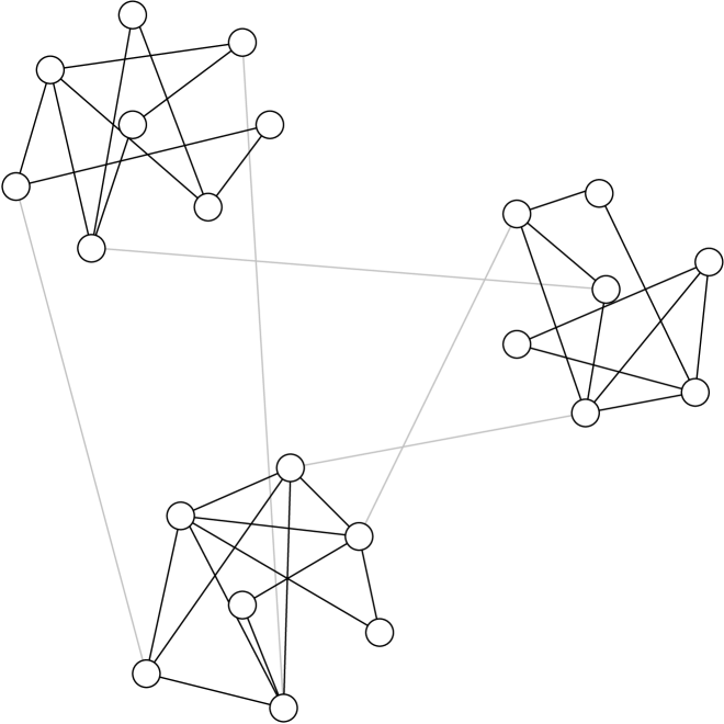
Figure 1: A figurative sketch of a network possessing community structure of the type discussed here.

A long-standing goal among social network analysts has been to find ways of analysing network data to reveal the structure of the underlying communities that they represent. It is commonly supposed that the actors in most social networks divide themselves naturally into groups of some kind, such that the density of ties within groups is higher than the density of ties between them. A sketch of a network with such community structure is shown in Fig. 1.

It is a matter of common experience that social networks do contain communities. We look around ourselves and see that we belong to this clique or that, that we have a circle of close friends and others whom we know less well, that there are groupings within our personal networks on the basis of interest, occupation, geographical location and so forth. This does not however guarantee that a network contains community structure of type that we are considering here. It would be perfectly possible for each person in a network to have a well-defined set of close acquaintances, their own personal network neighbourhood, but for the network neighbourhoods of different people to overlap only partially, so that the network as a whole is quite homogeneous, with no clear communities emerging from the pattern of vertices and edges. A network model showing precisely this type of structure has been proposed and studied recently by Kleinberg [17]. Our purpose in this section will be to investigate methods for detecting whether true community structure does exist in networks and for extracting the communities, and to apply those methods to particular networks. As we will see, the early intuition of the sociologists was correct, and many of the networks studied, including non-social networks, do possess large-scale inhomogeneity of precisely the type that would indicate the presence of community divisions.

The problem then is to take a network, specified in the simplest case by a list of $n$ vertices joined in pairs by $m$ edges, and from this structure to extract a set of communities—non-overlapping subsets of vertices that are, in some sense, tightly knit, having stronger within-group connections than between-group connections. The traditional, and still most common, method for detecting structure of this kind is the method of “hierarchical clustering” [15, 16]. In this method one defines a connection strength for each pair of vertices in the network, i.e., $\mbox{$\frac{1}{2}$}n(n-1)$ numbers that represent a distance or weight for the connection between each pair. (In some versions of the method not all pairs are assigned a connection strength, in which case those that are not can be assumed to have a connection strength of zero.) Examples of possible definitions for the strengths include geodesic (shortest path) distances between pairs, or their inverses if one wants a measure that increases when pairs are more closely connected, counts of numbers of vertex- or edge-independent paths between pairs (“maxflow” methods) or weighted counts of total numbers of paths between pairs (adjacency matrix methods).

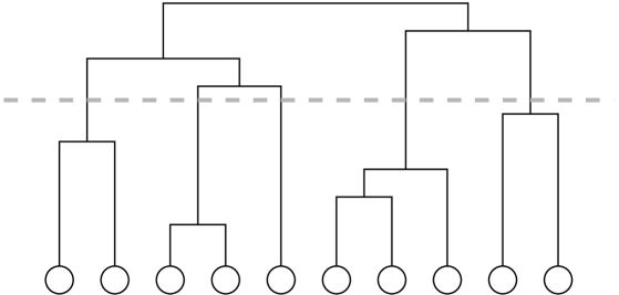
Figure 2: An example of a dendrogram showing the hierarchical clustering of ten vertices. A horizontal cut through the dendrogram, such as that denoted by the dotted line, splits the vertices into a set of communities, five in this case.

Then, starting with the $n$ vertices but no edges between them, one joins vertices together in decreasing order of the weights of vertex pairs, ignoring the edges of the original network. One can pause at any stage in this process and observe the pattern of components formed by the connections added so far, which are taken to be the communities of the network at that stage. The heirarchical clustering method thus defines not just a single decomposition of the network into communities, but a nested hierarchy of possible decompositions, having varying numbers of communities. This hierarchy can be represented as a tree or “dendrogram”, an example of which is shown in Fig. 2. A horizontal cut through the dendrogram at any given height, such as that denoted by the dotted line in Fig. 2, splits the tree into the communities for the corresponding stage in the hierarchical clustering process. By varying the height of the cut, one can arrange for the number of communities to take any desired value.

The construction of dendrograms is a popular technique for the analysis of network data, particularly within the sociological community. Software packages for network analysis, such as Pajek and UCInet, incorporate hierarchical clustering as a standard feature: for any network one can calculate a huge variety of vertex–vertex weights of different types and construct the corresponding dendrogram for any of them. The method however has some problems. There are many cases in which networks have rather obvious community structure, but hierarchical clustering fails to find it. One particular pathology that is frequently observed is that peripheral vertices tend to get disconnected from the bulk of the network, rather than being associated with the groups or communities that they are primarily attached to. For example, if a vertex is connected to the rest of the network by only a single edge, then presumably, were one to assign it to a community, it would be assigned to the community that the single edge leads to. In many cases, however, the hierarchical clustering method will declare the vertex instead to be a single-vertex community in its own right, in disagreement with our intuitive ideas of community structure.

In a recent paper therefore [12] we have proposed an alternative method for detecting community structure, based on calculations of so-called edge betweenness for vertex pairs. As we will see, this method detects the known community structure in a number of networks with remarkable accuracy.

2.1 Edge betweenness and community detection

Freeman [18] proposed a measure of centrality for the actors in a social network which he called “betweenness”. The betweenness of an actor is defined to be the number of shortest paths between pairs of vertices that pass through that actor. In cases where the number $p$ of shortest paths between a vertex pair is greater than one, each path is given an equal weight of $1/p$. Trivial algorithms for calculating betweenness take ${\rm O}(mn^{2})$ time to calculate betweenness for all vertices, or ${\rm O}(n^{3})$ time on a sparse graph (i.e., one in which the number of edges per vertex is constant in the limit of large graph size). This makes the calculation prohibitively costly on large networks. Recently however, two new algorithms have been proposed [19, 20] that both allow the same calculation to be performed faster, in time ${\rm O}(mn)$, or ${\rm O}(n^{2})$ on a sparse graph, by eliminating needless recalculations of geodesic paths. The betweenness of a vertex gives an indication, as the name implies, of how much the vertex is “between” other vertices. If, for example, information (or anything else) spreads through a network primarily by following shortest paths, then betweenness scores will indicate through which vertices most information will flow on average. The vertices with highest betweenness are also those whose removal will result in an increase to the geodesic distance between the largest number of other vertex pairs.

Here we consider an extension of Freeman’s betweenness to the edges in a network. The betweenness of an edge is defined to be the number of shortest paths between pairs of vertices that run along that edge, with paths again being given weights $1/p$ when there are $p>1$ between a given pair of vertices. In fact, the concept of edge betweenness actually appears to predate Freeman’s work on vertex betweenness, having appeared in an obscure technical report by an Amsterdam mathematician some years earlier [21]. Edge betweenness has received very little attention in other literature until recently, but it provides us with an excellent measure of which edges in a network lie between different communities. In a network with strong community structure—groups of vertices with only a few inter-group edges joining them—at least some of the inter-group edges will necessarily receive high edge betweenness scores, since they must carry the geodesic paths between vertex pairs that lie in different communities. This implies that eliminating edges with high edge betweenness from a graph will remove the inter-group edges, and hence split the graph efficiently into its different groups. This is the principle behind our method for the detection of community structure. Our algorithm is as follows.

1. We calculate the edge betweenness of every edge in the network.

2. We remove the edge with the highest betweenness score, or randomly choose one such if more than one edge ties for the honour.

3. We recalculate betweenness scores on the resulting network and repeat from step 2 until no edges remain.

The recalculation in step 3 is crucial to the method’s success. When there is more than one inter-group edge between two groups of vertices, there is no guarantee that both will receive high betweenness scores; in some cases most geodesic paths will flow along one edge and only that one will receive a high score. Recalculation ensures that at some stage in the working of the algorithm each inter-group edge receives a high score and thus gets removed.

The calculation of all edge betweennesses takes time ${\rm O}(mn)$, and its repetition for all $m$ edges thus gives the algorithm a worst-case running time of ${\rm O}(m^{2}n)$, or ${\rm O}(n^{3})$ on a sparse graph. The results of the algorithm can be represented as a dendrogram, just as in traditional hierarchical clustering, although one should be aware that the construction of the tree is not logically the same: the recalculation of the betweennesses after each edge removal means that there is no single function that can be defined for each edge in the initial graph such that the resulting dendrogram is the representation of a hierarchical clustering construction carried out using that function.

2.2 Examples

Here we give three examples of the application of our community structure finding algorithm to different networks. The first example is a set of computer generated graphs, specifically created to test the algorithm. We created a large number of graphs of 128 vertices each, divided into four groups of 32 vertices. Edges were placed at random between vertices within the same group with probability $p_{\rm in}$ and between vertices in different groups with probability $p_{\rm out}$, with the values of $p_{\rm in}$ and $p_{\rm out}$ chosen to make the average degree of a vertex equal to 16, and $p_{\rm out}\leq p_{\rm in}$. These graphs were then fed into our community structure algorithm, and we measured what fraction of the vertices were correctly classified into their communities as a function of the ratio of $p_{\rm in}$ to $p_{\rm out}$, or equivalently the mean number $z_{\rm out}$ of edges from a vertex to vertices in other communities. The results are shown in Fig. 3. As the figure shows, the algorithm performs almost perfectly for values of $z_{\rm out}$ up to about 6. Beyond this point, as $z_{\rm out}$ approaches the value of 8 at which each vertex has as many inter-group edges as intra-group ones, the fraction of successfully classified vertices falls off sharply.

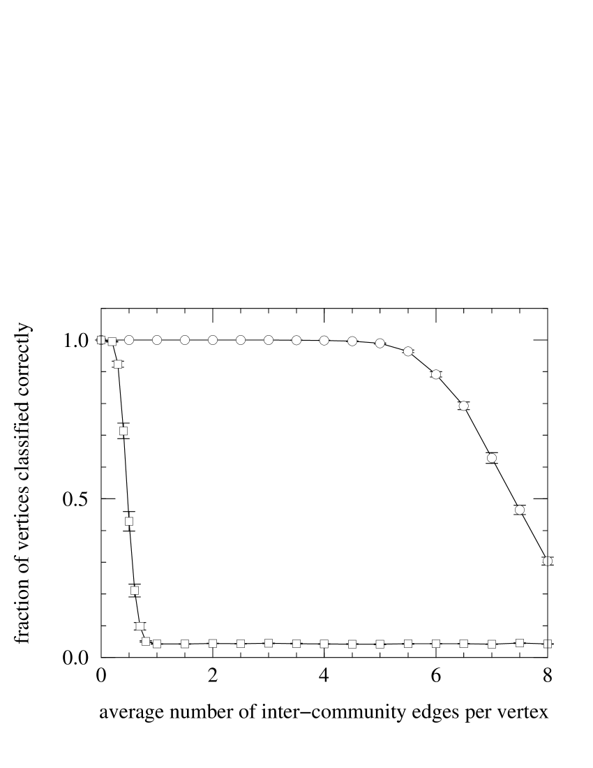
Figure 3: The fraction of vertices correctly classified in applications of community structure finding algorithms to the computer-generated graphs described in the text. The circles are results for the method presented in this paper and the squares are for the standard hierarchical clustering method, using a maximum-flow measure of connection strength between vertex pairs. Each point is an average over 100 realizations of the graphs.

On the same plot we also show the performance of a standard hierarchical clustering algorithm based on edge-independent path counts (maxflow) on the same set of random graphs. As the figure shows, the traditional method is far inferior to our new algorithm in finding the known community structure.

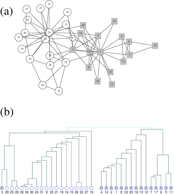
Figure 4: (a) The friendship network given by Zachary [22] for his karate club study. Grey squares represent individuals who in the fission of the club sided with the club’s instructor, while open circles represent individuals who sided with the club’s president. (b) The dendrogram representing the community divisions found by our method for this network, with the same colouring scheme for the vertices.

For our second example, we move to real-world network data. In 1977, Wayne Zachary published the results of an ethnographic study he had conducted of social interactions between 34 members of a karate club at an American university [22]. He recorded social contacts between members of the club over a two year period and published his results in the form of social networks. Fortuitously there arose, during the course of the study, a dispute between the two leaders of the club, the karate teacher and the club’s president, over whether to raise the club’s fees. Ultimately, the dispute resulted in the departure of the karate teacher and his starting another club of his own, taking with him about a half of the original club’s members. Here we analyse a network constructed by Zachary of friendships between club members before the split occurred. We compare the predictions of our community-finding algorithm applied to this network with the known lines along which the club divided. Our results are shown in Fig. 4.

In panel (a) of the figure we show the original network, with the grey squares representing the faction that ultimately sided with the teacher (who is vertex number 1), and the open circles the faction that sided with the club’s president (vertex number 34). In panel (b) we show the dendrogram output by our algorithm for this network. As the figure shows, the algorithm again performs nearly perfectly, with only one vertex, vertex number 3, being misclassified. (Inspection of panel (a) reveals that vertex 3 is in fact precisely caught in the middle of the network between the two factions, and so it is not entirely surprising that this vertex was misclassified.) Bear in mind that the network in this example was recorded before the fission of the club, so that the results of panel (b) are in some sense a prediction of events that were, at that time, yet to occur.

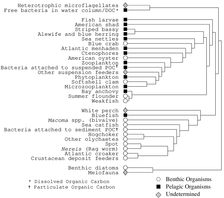
Figure 5: The dendrogram found by our method for Baird and Ulanowicz’s food web of marine organisms in the Chesapeake Bay [23].

Finally, for our third example, we take a network for which we do not have any strong presuppositions about a “correct” division into communities. This example is a true experiment to see what information the algorithm can give us about a network whose structure is not wholly understood. The network in question is a food web, the web of trophic interactions (who eats whom) of marine organisms living in the Chesapeake Bay. The network was assembled by Baird and Ulanowicz [23] and contains 33 vertices representing the ecosystem’s most prominent taxa. The edges in a food web are, technically, directed; they can be thought of as pointing from prey to their predators, thus indicating the direction of energy (or carbon) flow up the food chain. Here however we have ignored the directed nature of the network, considering the edges merely to be undirected indicators of trophic interaction between taxon pairs.

The dendrogram produced for this food web by our community structure algorithm is shown in Fig. 5. As we can see, the algorithm splits the network into two principle communities and a couple of smaller peripheral ones. We have shaded the vertices in the dendrogram to show which taxa are surface dwellers in the bay (pelagic species) and which bottom dwellers (benthic species). A few species are of undetermined status. It is clear that our algorithm has in this case primarily extracted from the network the distinction between pelagic and benthic taxa. Thus our results appear to imply that the food web in question can be split roughly into separate surface- and bottom-dwelling subsystems, with relatively weak interaction between the two. A small number of benthic species are found to belong more strongly to the pelagic community than to the benthic one, perhaps indicating that a simple classification of species by where they live is not telling the whole story for this system. The results of our analysis might also be helpful in assigning a type to the undetermined species in the network.

3 Origins of community structure and assortative mixing

There is certainly more than one possible explanation for the presence of community structure in a network, and different explanations may be appropriate to different networks. In the case of a social network, for example, Jin et al. [24] have shown that communities can arise as a result of the growth dynamics of a network. If an acquaintance network grows by the introduction of pairs of people to one another by a mutual acquaintance, then an initial chance acquaintance with a member of a certain community will lead to introductions to other members of that community, so that one ultimately becomes linked to many of the community’s members and so becomes a member oneself. Using a simple computer model of this process, Jin et al. found that even networks with no initial community structure quickly develop such structure over time. One can think of this as a mechanism for the development of cliquishness in social networks.

This mechanism however is quite specific to social networks and could not be easily applied, for example, to the food web studied in the last section. It also completely ignores any personal attributes of the actors involved or affinities between actor pairs. A more general and perhaps more convincing explanation for community formation, which takes these things into account, is that of assortative mixing, which is the tendency for nodes in a network to form connections preferentially to others that are like them in some way.

		women
		black	hispanic	white	other	$a_{i}$
men	black	0.258	0.016	0.035	0.013	0.323
	hispanic	0.012	0.157	0.058	0.019	0.247
	white	0.013	0.023	0.306	0.035	0.377
	other	0.005	0.007	0.024	0.016	0.053
$b_{i}$		0.289	0.204	0.423	0.084

Table 1: The mixing matrix $e_{ij}$ and the values of $a_{i}$ and $b_{i}$ for sexual partnerships in the San Francisco study described in the text. After Morris [25].

An example of assortative mixing in social networks is mixing by race. Table 1 shows data from the AIDS in Multiethnic Neighborhoods study [26], on mixing by race among sexual partners in the city of San Francisco, California. This part of the study focused on heterosexual partnerships, and the rows and columns of the matrix represent men and women in such partnerships, grouped by their (self-identified) race. Diagonal elements of the matrix represent the fraction of survey respondents in partnerships with members of their own group, and off-diagonal those in partnerships with members of other groups. Inspection of the figures shows that the matrix has considerably more weight along its diagonal than off it, indicating that assortative mixing does take place in this network. One might well expect mixing of this type to result in divisions within the community along lines of race, and we will show shortly that, within the context of simulations of network formation, assortative mixing can indeed give rise to community structure.

The amount of assortative mixing in a network can be characterized by measuring how much of the weight in the mixing matrix falls on the diagonal, and how much off it. Let us define $e_{ij}$ to be the fraction of all edges in a network that join a vertex of type $i$ to a vertex of type $j$. In the case of the matrix of Table 1, where the ends of an edge always attach to one man and one woman, we also specify which index corresponds to which type of end, which makes $e_{ij}$ asymmetric. For example, we could specify that the first index $i$ represents the man and the second $j$ the woman. For networks in which there is no corresponding distinction, $e_{ij}$ will be symmetric. The matrix should also satisfy the sum rules

$$\sum_{ij}e_{ij}=1,\qquad\sum_{j}e_{ij}=a_{i},\qquad\sum_{i}e_{ij}=b_{j},$$ (1)

where $a_{i}$ and $b_{i}$ are the fraction of each type of end of an edge that is attached to vertices of type $i$. The values of $a_{i}$ and $b_{i}$ for the San Francisco study are also shown in Table 1. On graphs where there is no distinction between the ends of edges, we will have $a_{i}=b_{i}$.

Now we can define a quantitative measure $r$ of the level of assortative mixing in the network thus [14]:

$$r={\sum_{i}e_{ii}-\sum_{i}a_{i}b_{i}\over 1-\sum_{i}a_{i}b_{i}}={\mathop{\rm Tr}\mathbf{e}-||\,\mathbf{e}^{2}\,||\over 1-||\,\mathbf{e}^{2}\,||},$$ (2)

where $\mathbf{e}$ is the matrix whose elements are the $e_{ij}$, and the notation $||\,\mathbf{x}\,||$ indicates the sum of the elements of the matrix $\mathbf{x}$. We call the quantity $r$ the “assortativity coefficient”. It takes the value 1 in a perfectly assortative network, since in that case the entire weight of the matrix $\mathbf{e}$ lies along its diagonal and $\sum_{i}e_{ii}=1$. Conversely, if there is no assortative mixing at all, then $e_{ij}=a_{i}b_{j}$ for all $i,j$ and $r=0$. Networks can also be disassortative: vertices may associate preferentially with others of different types—the “opposites attract” phenomenon. In that case, $r$ will take a negative value.

One can certainly imagine that assortative mixing might apply in other types of networks as well. For example, we saw in Section 2.2 that a food web of marine organisms apparently divided into communities along lines of location—which species were surface dwellers (pelagic) and which bottom dwellers (benthic). It seems reasonable to hypothesize that the evolution of new predatory relationships between species is biased by the location of those species’ living quarters, and hence that the network structure would indeed reflect the pelagic/benthic division as a result of assortative mixing by location.

We can test our hypothesis that assortative mixing could be responsible for community formation in networks by computer simulation. Given a mixing matrix of the type shown in Table 1, we can create a random network with the corresponding mixing pattern and any desired degree distribution by the following algorithm.

1. First we choose degree distributions $p_{k}^{(i)}$ for each vertex type $i$. The quantity $p_{k}^{(i)}$ here denotes the probability that a randomly chosen vertex of type $i$ will have degree $k$. We can also calculate the mean degree $z_{i}=\sum_{k}kp_{k}^{(i)}$ for each vertex type.

2. Next we choose a size for our graph in terms of the number $m$ of edges and draw $m$ edges from the desired distribution $e_{ij}$. We count the number of ends of edges of each type $i$, to give the sums $m_{i}$ of the degrees of vertices in each class, and we calculate the expected number $n_{i}$ of vertices of each type from $n_{i}=m_{i}/z_{i}$ (rounded to the nearest integer).

3. We draw $n_{i}$ vertices from the desired degree distribution $p_{k}^{(i)}$ for type $i$. Normally the degrees of these vertices will not sum exactly to $m_{i}$ as we want them to, in which case we choose one vertex at random, discard it, and draw another from the distribution $p_{k}^{(i)}$, repeating until the sum does equal $m_{i}$.

4. We pair up the $m_{i}$ ends of edges of type $i$ at random with the vertices we have generated, so that each vertex has the number of attached edges corresponding to its chosen degree.

5. We repeat from step 3 for each vertex type.

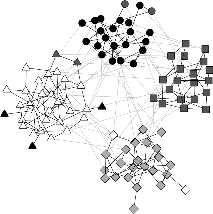
Figure 6: A network generated using the mixing matrix of Eq. (3) and a Poisson degree distribution with mean $z=5$. The four different shades of vertices represent the four types, and the four shapes represent the communities discovered by the community-finding algorithm of Section 2.1. The placement of the vertices has also been chosen to accentuate the communites and show where the algorithm fails. As we can see, the correspondence between vertex type and the detected community structure is very close; only nine of the 100 vertices are misclassified.

We have used this algorithm to generate example networks with desired levels of assortative mixing. For example, Fig. 6 shows an undirected network of $n=100$ vertices of four different types, generated using the symmetric mixing matrix

$$\mathbf{e}=\begin{pmatrix}0.18&0.02&0.01&0.03\\ 0.02&0.20&0.03&0.02\\ 0.01&0.03&0.16&0.01\\ 0.03&0.02&0.01&0.22\\ \end{pmatrix},$$ (3)

which gives a value of $r=0.68$ for the assortativity coefficient. A simple Poisson degree distribution with mean $z=5$ was used for all vertex types. The graph was then fed into the community finding algorithm of Section 2.1 and a cut through the resulting dendrogram performed at the four-community level. The communities found are shown by the four shapes of vertices in the figure and correspond very closely to the real vertex type designations, which are represented by the four different vertex shades. In other words, by introducing assortative mixing by vertex type into this network, we have created vertex-type communities that register in our community finding algorithm in exactly the same way as communities in naturally occurring networks. This strongly suggests that assortative mixing could indeed be an explanation for the occurrence of such communities, although it is worth repeating that other explanations are also possible.

4 Other types of assortative mixing

Assortative mixing can depend on vertex properties other than the simple enumerative properties discussed in the preceding section. For example, we can also have assortative mixing by scalar characteristics, either discrete or continuous. A classic example of such mixing, much studied in the sociological literature, is acquaintance matching by age. In many contexts, people appear to prefer to associate with others of approximately the same age as themselves. For example, consider Fig. 7, which shows the ages at marriage of the male and female members of 1141 married couples drawn from the US National Survey of Family Growth [27]. Each point in the figure represents one couple, its position along the horizontal and vertical axes corresponding to the ages of the husband and wife respectively. The study was based on interviews with women, and was limited to those of childbearing age, so the vertical axis cuts off around 40. Also only the first marriage for each woman interviewed is shown, even if she married more than once. Despite these biases however, the figure reveals a clear trend: people prefer to marry others of an age close to their own.

Figure 7: Scatter plot of the ages at first marriage of 1141 women interviewed in the 1995 National Survey of Family Growth, and their spouses.

It is perhaps stretching a point a little to consider first marriage ties between couples as forming a social network, since people have at most one first marriage and hence would have a maximum degree of one within the network. Here, however, we consider marriage age as a proxy for the ages of sexual partners in general, and conjecture that a similar age preference will be seen in non-married partners also. A recent study by Garfinkel et al. [28] appears to support this conjecture.

Assortative mixing according to scalar characteristics can result in the formation of communities, just as in the case of discrete characteristics. One could have separate communities formed of old and young people, for instance. However, it is also possible that we do not get well-defined communities, but instead get an overlapping set of groups with no clear boundaries, ranging for example from low age to high age. In the sociological literature such a continuous gradation of one community into another is called “stratification” of the network.

As with assortative mixing on discrete characteristics, one can define an assortativity coefficient to quantify the extent to which mixing is biased according to scalar vertex properties. To do this, we define $e_{xy}$ to be the fraction of edges in our network that connect a vertex of property $x$ to another of property $y$. The matrix $e_{xy}$ must satisfy sum rules as before, of the form

$$\sum_{xy}e_{xy}=1,\qquad\sum_{y}e_{xy}=a_{x},\qquad\sum_{x}e_{xy}=b_{y},$$ (4)

where $a_{x}$ and $b_{y}$ are, respectively, the fraction of edges that start and end at vertices with ages $x$ and $y$. Then the appropriate definition for the assortativity coefficient is

$$r={\sum_{xy}xy(e_{xy}-a_{x}b_{y})\over\sigma_{a}\sigma_{b}},$$ (5)

where $\sigma_{a}$ and $\sigma_{b}$ are the standard deviations of the distributions $a_{x}$ and $b_{y}$. The reader will no doubt recognize this definition of $r$ as the standard Pearson correlation coefficient for the quantities $x$ and $y$. It takes values in the range $-1\leq r\leq 1$ with $r=1$ indicating perfect assortative mixing, $r=0$ indicating no correlation between $x$ and $y$, and $r=-1$ indicating perfect disassortative mixing, i.e., perfect anticorrelation between $x$ and $y$.

If we take the marriage data from Fig. 7, for example, and feed it into Eq. (5), we find that $r=0.57$, indicating once again that mixing is strongly assortative (as is in any case obvious from the figure).

Mixing could also depend on vector or even tensor characteristics of vertices. One example would be mixing by geographical location, which could be regarded as a two-vector. It seems highly likely that if one were to record both acquaintance patterns and geographical location for actors in a social network, one would discover that acquaintance is strongly dependent on geography, with people being more likely to know others who live in the same part of the world as themselves.

4.1 Mixing by vertex degree

We will spend the rest of this article examining one particular case of mixing according to a scalar vertex property, that of mixing by vertex degree, which has been studied for some time in the social networks literature and has recently attracted attention in the mathematical and physical literature also. Krapivsky and Redner [29] for instance found in studies of the preferential attachment model of Barabási and Albert [30] that edges did not fall between vertices independent of their degrees. Instead there was a higher probability to find some degree combinations at the ends of edges than others. Pastor-Satorras et al. [31] showed for data on the structure of the Internet at the level of autonomous systems that the degrees of adjacent vertices were anticorrelated, i.e., that high-degree vertices prefer to attach to low-degree vertices, rather than other high-degree ones—the network is disassortative by degree. To demonstrate this, they measured the mean degree degree $\langle k_{\rm nn}\rangle$ of the nearest-neighbours of a vertex, as a function of that vertex’s degree $k$. They found that $\langle k_{\rm nn}\rangle$ decreases with increasing $k$, approximately as $k^{-1/2}$. That is, the mean degree of your neighbours goes down as yours goes up. Maslov and Sneppen [32] have offered an explanation of this result in terms of ensembles of graphs in which double edges between vertices are forbidden. Maslov and Sneppen also showed in a separate paper [33] that the protein interaction network of the yeast S. Cerevisiae displays a similar sort of disassortative mixing.

An alternative way to quantify assortative mixing by degree in a network is to use an assortativity coefficient of the type described in the previous section [13]. Let us define $e_{jk}$ to be the fraction of edges in a network that connect a vertex of degree $j$ to a vertex of degree $k$. (As before, if the ends of an edge connect different types of vertices, then the matrix will be asymmetric, otherwise it will be symmetric.) In fact, we define $j$ and $k$ to be the “excess degrees” of the two vertices, i.e., the number of edges incident on them less the one edge that we are looking at at present. In other words, $j$ and $k$ are one less than the total degrees of the two vertices. This designation turns out to be mathematically convenient for many developments. If the degree distribution of the network as a whole is $p_{k}$, then the distribution of the excess degree of the vertex at the end of a randomly chosen edge is

$$q_{k}={(k+1)p_{k+1}\over z},$$ (6)

where $z=\sum_{k}kp_{k}$ is the mean degree [34]. Then one can define the assortativity coefficient to be

$$r={\sum_{jk}jk(e_{jk}-q_{j}q_{k})\over\sigma_{q}^{2}},$$ (7)

where $\sigma_{q}$ is the standard deviation of the distribution $q_{k}$. On a directed or similar network, where the ends of an edge are not the same and $e_{jk}$ is asymmetric, this generalizes to

$$r={\sum_{jk}jk(e_{jk}-q^{a}_{j}q^{b}_{k})\over\sigma_{a}\sigma_{b}},$$ (8)

where $\sigma_{a}$ and $\sigma_{b}$ are the standard deviations of the distributions $q^{a}_{k}$ and $q^{b}_{k}$ for the two types of ends. (The measure introduced by Pastor-Satorras et al. [31] can also be expressed simply in terms of the matrix $e_{jk}$: it is $\langle k_{\rm nn}\rangle=\sum_{j}je_{jk}/q_{k}$. Maslov and Sneppen [33, 32] gave entire plots of the raw $e_{jk}$, using colours to code for different values. These plots are however rather difficult to interpret by eye.)

	network	type	size $n$	assortativity $r$	ref.
social	physics coauthorship	undirected	$52\,909$	$\phantom{-}0.363$	a
	biology coauthorship	undirected	$1\,520\,251$	$\phantom{-}0.127$	a
	mathematics coauthorship	undirected	$253\,339$	$\phantom{-}0.120$	b
	film actor collaborations	undirected	$449\,913$	$\phantom{-}0.208$	c
	company directors	undirected	$7\,673$	$\phantom{-}0.276$	d
	email address books	directed	$16\,881$	$\phantom{-}0.092$	e
technol.	Internet	undirected	$10\,697$	$-0.189$	f
	World-Wide Web	directed	$269\,504$	$-0.067$	g
	software dependencies	directed	$3\,162$	$-0.016$	h
biological	protein interactions	undirected	$2\,115$	$-0.156$	i
	metabolic network	undirected	$765$	$-0.240$	j
	neural network	directed	$307$	$-0.226$	k
	marine food web	directed	$134$	$-0.263$	l
	freshwater food web	directed	$92$	$-0.326$	m

Table 2: Size $n$ and degree assortativity coefficient $r$ for a number real-world networks. Social networks: coauthorship networks of (a) physicists and biologists [35] and (b) mathematicians [36]; (c) collaborations (co-starring relationships) of film actors [11, 37]; (d) directors of Fortune 1000 companies for 1999, in which two directors are connected if they sit on the board of directors of the same company [38, 37]; (e) network of email address books of computer users [39]. Technological networks: (f) network of direct peering relationships between autonomous systems on the Internet, April 2001 [40]; (g) network of hyperlinks between pages in the World-Wide Web domain nd.edu circa 1999 [41]; (h) network of dependencies between software packages in the GNU/Linux operating system [14]. Biological networks: (i) protein–protein interaction network in the yeast S. Cerevisiae [42]; (j) metabolic network of the bacterium E. Coli [43]; (k) neural network of the nematode worm C. Elegans [44, 11]; tropic interactions between species in the food webs of (l) Ythan Estuary, Scotland [45] and (m) Little Rock Lake, Wisconsin [46].

In Table 2 we show values of $r$ measured for a variety of different real-world networks. The networks shown are divided into social, technological and biological networks, and a particularly striking feature of the table is that the values of $r$ for the social networks are all positive, indicating assortative mixing by degree, while those for the technological and biological networks are all negative, indicating disassortative mixing. It is not clear at present why this should be, although explanations for the observed mixing behaviours have been proposed in some specific cases [32, 14].

As with the mixing by discrete enumerative characteristics discussed in Section 3, we can also investigate the effects of assortative mixing by looking at computer generated networks with particular types of mixing. Unfortunately, no simple algorithm exists for generating graphs mixed by vertex degree analogous to that of Section 3 (see Refs. [47] and [14]) and one is forced to resort to Monte Carlo generation of graphs using Metropolis–Hastings type algorithms of the sort widely used for graph generation in mathematics and quantitative sociology. Such algorithms however are straightforward to implement. For the present case, we take the simple example form

$$e_{jk}=\mathcal{N}{\rm e}^{-(j+k)/\kappa}\biggl{[}{j+k\choose j}p^{j}q^{k}+{j+k\choose k}p^{k}q^{j}\biggr{]},$$ (9)

where $p+q=1$, $\kappa>0$, and $\mathcal{N}=\mbox{$\frac{1}{2}$}(1-{\rm e}^{-1/\kappa})$ is a normalizing constant. This means that the distribution of the sum $j+k$ of the excess degrees at the ends of an edge falls off as a simple exponential, while that sum is distributed between the two ends binomially, the parameter $p$ controlling the assortative mixing. For values of $p$ ranging from 0 to $\frac{1}{2}$ we get various values of the assortativity $r$, both positive and negative, passing through zero at $p_{0}=\mbox{$\frac{1}{2}$}-\frac{1}{4}\sqrt{2}=0.1464\ldots$

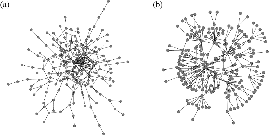
Figure 8: The giant component of two graphs generated using a Monte Carlo procedure with edge distribution given by Eq. (9) with $\kappa=10$ and (a) $p=0.5$ and (b) $p=0.05$.

As an example, we show in Fig. 8 the giant components of two graphs of this type generated using the Monte Carlo method. One of them, graph (a), is assortatively mixed by degree, while the other, graph (b), is disassortatively mixed. The difference between the two is clear to the eye. In the first case, because the high degree vertices prefer to attach to one another, there is a central “core” to the network, composed of these high-degree vertices, and a straggling periphery of low-degree vertices around it. In epidemiology a dense central portion of this type is called a “core group” and is thought to be capable of acting as a reservoir for disease, keeping diseases circulating even when the density of the network as a whole is too low to maintain endemic infection. In social network analysis one also talks of “core/periphery” distinctions in networks, another concept that mirrors what we see here. In the second graph, which is disassortative, a contrasting picture is evident: the high-degree vertices prefer not to associate with one another, and are as a result scattered widely over the network, producing a more uniform appearance.

Figure 9: The size of the giant component as a function of graph size for graphs with the edge distribution given in Eq. (9), for three different values of the parameter $p$, which controls the assortativity. The points are simulation results for graphs of $N=100\,000$ vertices while the solid lines are the analytic solution for the same quantity given by Newman [13]. Each point is an average over ten graphs; the resulting statistical errors are smaller than the symbols. The values of $p$ are 0.5 (circles), $p_{0}=0.146\ldots$ (squares), and $0.05$ (triangles).

To shed more light on the effects of assortativity, we show in Fig. 9 the size of the largest component in networks of this type as the degree distribution parameter $\kappa$ is varied, for various values of $p$. For low values of $\kappa$ the mean degree of the network is small, and the resulting density of edges is too low to produce percolation in the network, so there is no giant component. As $\kappa$ increases, however, there comes a point, clearly visible on the plot, at which the edge density is great enough to form a giant component. Figure 9 reveals two interesting features of this transition. First, the position of the transition, the value of the parameter $\kappa$ at which it takes place, is smaller in assortatively mixed networks than in disassortative ones. In other words, it appears that the presence of assortativity in the degree correlation pattern allows the network to percolate more easily. This result is intuitively reasonable: the core group of the assortative network seen in Fig. 8a has a higher density of edges than the network as a whole and so one would expect percolation to take place in this region before it would in a network with the same average density but no core group.

Second, the figure shows that, even though the assortative network percolates more easily than its disassortative counterpart, its largest component does not grow as large as that of the disassortative network in the limit where $\kappa$ becomes large. This too can be understood in simple terms: percolation occurs more easily when there is a core group, but is also largely confined to that core group and so does not spread to as large a portion of the network as it would in other cases.

In epidemiological terms, one could think of these two results as indicating that assortative networks will support the spread and persistence of a disease more easily than disassortative ones, because they possess a core group of connected high-degree vertices. But the disease is also restricted mostly to that core group. In a disassortative network, although percolation and hence epidemic disease requires a denser network to begin with, when it does happen it will affect a larger fraction of the network, because it is not restricted to a core group.

5 Conclusions

In this article we have examined two related properties of networks: community structure and assortative mixing. We have described a new algorithm for finding groups of tightly-knit vertices within networks—communities in our nomenclature—which is based on the calculation of an “edge betweenness” index for network edges. The algorithm appears to be successful at detecting known community structure in various example networks, and we have found that a number of real-world networks do indeed possess community structure to a greater or lesser degree.

Turning to possible explanations for this structure we have suggested that assortative mixing, the preferential association of vertices in a network with others that are like them in some way, is one possible mechanism for community formation. We have defined a measure of the strength of assortative mixing and applied it, for example, to data on mixing by race in social networks, showing that there is strong assortativity in this case, at least for the survey data that we have examined. We have also given a simple algorithm for creating networks with assortative mixing according to discrete characteristics imposed upon the vertices, and used it to generate example networks which, when fed into our community detection algorithm, reveal strong community structure similar to that seen in the real-world data. This lends some conviction to the theory that assortative mixing could, at least in some cases, be a contributing factor in the formation of communities within networks.

We have also looked at assortative mixing by scalar characteristics of vertices, such as the age of individuals in a social network, and particularly vertex degree. By measuring mixing of the latter type for a variety of different networks, we have shown that social networks appear often to be assortatively mixed by degree, while technological and biological networks appear normally to be disassortative. Using computer generated model networks we have also shown that assortativity by vertex degree makes networks percolate more easily—they develop a giant component for a lower average edge density than a similar network with neutral or disassortative mixing. Conversely, however, disassortative networks tend to have larger giant components when they do develop. These findings have implications for epidemiology, for example: they imply that a disease spreading on a network that is assortatively mixed, as most social networks appear to be, would reach epidemic proportions more easily than on a disassortative network, but that the epidemic might ultimately affect fewer people than in the disassortative case.

Looking ahead, some obvious next steps in the studies presented here are the application of community finding algorithms to other networks, the study of mixing patterns in other networks, and theoretical investigations of the effects of assortative mixing and other network correlations on network structure and function, including for instance network resilience and network epidemiology. A number of authors have already started work on these problems [48, 49, 50, 51, 13, 14].

References

- [1] S. H. Strogatz, Exploring complex networks. Nature 410, 268–276 (2001).
- [2] R. Albert and A.-L. Barabási, Statistical mechanics of complex networks. Rev. Mod. Phys. 74, 47–97 (2002).
- [3] S. N. Dorogovtsev and J. F. F. Mendes, Evolution of networks. Advances in Physics 51, 1079–1187 (2002).
- [4] A. Broder, R. Kumar, F. Maghoul, P. Raghavan, S. Rajagopalan, R. Stata, A. Tomkins, and J. Wiener, Graph structure in the web. Computer Networks 33, 309–320 (2000).
- [5] P. Grassberger, On the critical behavior of the general epidemic process and dynamical percolation. Math. Biosci. 63, 157–172 (1983).
- [6] A. Barbour and D. Mollison, Epidemics and random graphs. In J. P. Gabriel, C. Lefevre, and P. Picard (eds.), Stochastic Processes in Epidemic Theory, pp. 86–89, Springer, New York (1990).
- [7] Y. Moreno, R. Pastor-Satorras, and A. Vespignani, Epidemic outbreaks in complex heterogeneous networks. Eur. Phys. J. B 26, 521–529 (2002).
- [8] J. M. Kleinberg, The small-world phenomenon: An algorithmic perspective. In Proceedings of the 32nd Annual ACM Symposium on Theory of Computing, pp. 163–170, Association of Computing Machinery, New York (2000).
- [9] L. A. Adamic, R. M. Lukose, A. R. Puniyani, and B. A. Huberman, Search in power-law networks. Phys. Rev. E 64, 046135 (2001).
- [10] D. J. Watts, P. S. Dodds, and M. E. J. Newman, Identity and search in social networks. Science 296, 1302–1305 (2002).
- [11] D. J. Watts and S. H. Strogatz, Collective dynamics of ‘small-world’ networks. Nature 393, 440–442 (1998).
- [12] M. Girvan and M. E. J. Newman, Community structure in social and biological networks. Proc. Natl. Acad. Sci. USA 99, 8271–8276 (2002).
- [13] M. E. J. Newman, Assortative mixing in networks. Preprint cond-mat/0205405 (2002).
- [14] M. E. J. Newman, Mixing patterns in networks. Preprint cond-mat/0209476 (2002).
- [15] S. Wasserman and K. Faust, Social Network Analysis. Cambridge University Press, Cambridge (1994).
- [16] J. Scott, Social Network Analysis: A Handbook. Sage Publications, London, 2nd edition (2000).
- [17] J. M. Kleinberg, Small world phenomena and the dynamics of information. In T. G. Dietterich, S. Becker, and Z. Ghahramani (eds.), Proceedings of the 2001 Conference on Neural Information Processing Systems, MIT Press, Cambridge, MA (2002).
- [18] L. Freeman, A set of measures of centrality based upon betweeness. Sociometry 40, 35–41 (1977).
- [19] M. E. J. Newman, Scientific collaboration networks: II. Shortest paths, weighted networks, and centrality. Phys. Rev. E 64, 016132 (2001).
- [20] U. Brandes, A faster algorithm for betweenness centrality. Journal of Mathematical Sociology 25, 163–177 (2001).
- [21] J. M. Anthonisse, The rush in a directed graph. Technical Report BN 9/71, Stichting Mathematicsh Centrum, Amsterdam (1971).
- [22] W. W. Zachary, An information flow model for conflict and fission in small groups. Journal of Anthropological Research 33, 452–473 (1977).
- [23] D. Baird and R. E. Ulanowicz, The seasonal dynamics of the Chesapeake Bay ecosystem. Ecological Monographs 59, 329–364 (1989).
- [24] E. M. Jin, M. Girvan, and M. E. J. Newman, The structure of growing social networks. Phys. Rev. E 64, 046132 (2001).
- [25] M. Morris, Data driven network models for the spread of infectious disease. In D. Mollison (ed.), Epidemic Models: Their Structure and Relation to Data, pp. 302–322, Cambridge University Press, Cambridge (1995).
- [26] J. A. Catania, T. J. Coates, S. Kegels, and M. T. Fullilove, The population-based AMEN (AIDS in Multi-Ethnic Neighborhoods) study. Am. J. Public Health 82, 284–287 (1992).
- [27] National Survey of Family Growth, Cycle V, 1995. U.S. Department of Health and Human Services, National Center for Health Statistics, Hyattsville, MD (1997).
- [28] I. Garfinkel, D. A. Glei, and S. S. McLanahan, Assortative mating among unmarried parents. Journal of Population Economics (in press).
- [29] P. L. Krapivsky and S. Redner, Organization of growing random networks. Phys. Rev. E 63, 066123 (2001).
- [30] A.-L. Barabási and R. Albert, Emergence of scaling in random networks. Science 286, 509–512 (1999).
- [31] R. Pastor-Satorras, A. Vázquez, and A. Vespignani, Dynamical and correlation properties of the Internet. Phys. Rev. Lett. 87, 258701 (2001).
- [32] S. Maslov and K. Sneppen, Pattern detection in complex networks: Correlation profile of the Internet. Preprint cond-mat/0205379 (2002).
- [33] S. Maslov and K. Sneppen, Specificity and stability in topology of protein networks. Science 296, 910–913 (2002).
- [34] M. E. J. Newman, Random graphs as models of networks. In S. Bornholdt and H. G. Schuster (eds.), Handbook of Graphs and Networks, Wiley-VCH, Berlin (2003).
- [35] M. E. J. Newman, The structure of scientific collaboration networks. Proc. Natl. Acad. Sci. USA 98, 404–409 (2001).
- [36] J. W. Grossman and P. D. F. Ion, On a portion of the well-known collaboration graph. Congressus Numerantium 108, 129–131 (1995).
- [37] M. E. J. Newman, S. H. Strogatz, and D. J. Watts, Random graphs with arbitrary degree distributions and their applications. Phys. Rev. E 64, 026118 (2001).
- [38] G. F. Davis, M. Yoo, and W. E. Baker, The small world of the corporate elite. Preprint, University of Michigan Business School (2001).
- [39] M. E. J. Newman, S. Forrest, and J. Balthrop, Email networks and the spread of computer viruses. Phys. Rev. E 66, 035101 (2002).
- [40] Q. Chen, H. Chang, R. Govindan, S. Jamin, S. J. Shenker, and W. Willinger, The origin of power laws in Internet topologies revisited. In Proceedings of the 21st Annual Joint Conference of the IEEE Computer and Communications Societies, IEEE Computer Society (2002).
- [41] R. Albert, H. Jeong, and A.-L. Barabási, Diameter of the world-wide web. Nature 401, 130–131 (1999).
- [42] H. Jeong, S. Mason, A.-L. Barabási, and Z. N. Oltvai, Lethality and centrality in protein networks. Nature 411, 41–42 (2001).
- [43] H. Jeong, B. Tombor, R. Albert, Z. N. Oltvai, and A.-L. Barabási, The large-scale organization of metabolic networks. Nature 407, 651–654 (2000).
- [44] J. G. White, E. Southgate, J. N. Thompson, and S. Brenner, The structure of the nervous system of the nematode C. Elegans. Phil. Trans. R. Soc. London 314, 1–340 (1986).
- [45] M. Huxham, S. Beany, and D. Raffaelli, Do parasites reduce the chances of triangulation in a real food web? Oikos 76, 284–300 (1996).
- [46] N. D. Martinez, Artifacts or atributes? Effects of resolution on the Little Rock Lake food web. Ecological Monographs 61, 367–392 (1991).
- [47] S. N. Dorogovtsev, J. F. F. Mendes, and A. N. Samukhin, Modern architecture of random graphs: Constructions and correlations. Preprint cond-mat/0206467 (2002).
- [48] P. Holme, M. Huss, and H. Jeong, Subnetwork hierarchies of biochemical pathways. Preprint cond-mat/0206292 (2002).
- [49] D. Wilkinson and B. A. Huberman, A method for finding communities of related genes. Preprint, Stanford University (2002).
- [50] M. Boguna, R. Pastor-Satorras, and A. Vespignani, Absence of epidemic threshold in scale-free networks with connectivity correlations. Preprint cond-mat/0208163 (2002).
- [51] A. Vazquez and Y. Moreno, Resilience to damage of graphs with degree correlations. Preprint cond-mat/0209182 (2002).