Pair distribution function in a two-dimensional electron gas

Abstract

We calculate the pair distribution function, $g(r)$, in a two-dimensional electron gas and derive a simple analytical expression for its value at the origin as a function of $r_{s}$. Our approach is based on solving the Schrödinger equation for the two-electron wave function in an appropriate effective potential, leading to results that are in good agreement with Quantum Monte Carlo data and with the most recent numerical calculations of $g(0)$. [C. Bulutay and B. Tanatar, Phys. Rev. B 65, 195116 (2002)] We also show that the spin-up spin-down correlation function at the origin, $g_{\uparrow\downarrow}(0)$, is mainly independent of the degree of spin polarization of the electronic system.

I Introduction

There has recently been a growth of interest in studying the pair distribution function, $g(r)$, in electron gas models,davoudi02 ; capurro02 ; gori01 ; Polini01 caused mainly by its relevance in non-local density functional theories. perdew96 ; chacon88 ; Gunnar79 The zero inter-electronic distance value, $g(r=0)$, also appears in the large wavevector and the high frequency limits of the electronic charge and spin response functions. niklasson ; zhu84 The importance of $g(r)$ lies in its connection with the electronic exchange and correlation of the electron gas model. Moreover, theoretical calculations of the pair distribution function can be directly compared with material properties since $g(r)$ is the Fourier transform of the static structure factor.

The pair-distribution function is the probability of finding a pair of electrons at a distance $r$ from each other. Therefore, the average number of electrons in a spherical shell centered on an given electron is $ng(r)\Omega_{D}r^{D-1}dr$, where $\Omega_{D}r^{D-1}dr$ is the volume of the D-dimensional shell and $n=N/V$ is the uniform electron density. At large distances, $g(r)$ approaches $1$, whereas near the origin, where the electron charge is depleted, it is small on account of the Pauli exclusion principle and the exchange and correlation effects associated with the Coulomb interaction.

The subject of this paper is an analysis of the pair correlation function dependence on the inter-electronic distance and electron density in a two dimensional, interacting, spin polarized electron system. Calculations of $g(r)$ in the two-dimensional paramagnetic electron gas have been reported by Freeman Freeman83 and Nagano et al.Nagano84 within the ladder approximation, by Tanatar and CeperleyTan89 using the diffusion quantum Monte Carlo method (QMC) and, more recently, by Bulutay and TanatarBulu02 using the hypernetted-chain approximation (CHNC). Moreover, an analytical expression of $g(0)$ has previously been derived by Polini et al.Polini01

In order to calculate $g(r)$, we follow the approach developed in three dimensional systems by Overhauser Over71 and further refined in Ref. Over95, and gori01, . This method is based on the relation between $g(r)$ and the two-electron scattering problem in an appropriately chosen effective potential which will be discussed in detail in the following sections. In addition to obtaining the variation of the pair distribution function as a function of the coupling-strength, $r_{s}$, and of the spin polarization, we also derive an analytic expression for $g(0)$:

$$g(0)=\frac{1}{2}\frac{1}{[1+0.6032~{}r_{s}+0.07263~{}r_{s}^{2}]^{2}}.$$ (1)

This expression is found to agree very well with the results of the most recent numerical calculations.Tan89 ; Bulu02 We also compare our results with the expression derived in Ref. Polini01, .

II Effective model for the pair distribution function

A spin-polarized electron gas is characterized, in equilibrium, by two parameters: the electronic density, or its equivalent $r_{s}$, and the polarization, $\zeta=(n_{\uparrow}-n_{\downarrow})/(n_{\uparrow}+n_{\downarrow})$, where $n_{\uparrow}$ and $n_{\downarrow}$ are the spin-up and -down electron densities. For this system, the pair distribution function is given by

$$g(\rho)=\frac{1}{4}[(1+\zeta)^{2}g_{\uparrow\uparrow}(\rho)+2(1-\zeta^{2})g_{\uparrow\downarrow}(\rho)+(1-\zeta)^{2}g_{\downarrow\downarrow}(\rho)],$$ (2)

where $g_{\sigma\sigma^{{}^{\prime}}}$ are the spin resolved pair distribution functions. Following Overhauser,Over95 $g_{\sigma\sigma^{{}^{\prime}}}$ can be related with the two-electron wave functions as:gori01

$$g_{\uparrow\downarrow}(\rho)=\frac{1}{2}\langle|\Psi_{\rm singlet}(\rho)|^{2}\rangle_{p_{\uparrow\downarrow}(k)}+\frac{1}{2}\langle|\Psi_{\rm triplet}(\rho)|^{2}\rangle_{p_{\uparrow\downarrow}(k)},$$ (3)

$$g_{\uparrow\uparrow}(\rho)=\langle|\Psi_{\rm triplet}(\rho)|^{2}\rangle_{p_{\uparrow\uparrow}(k)},$$ (4)

$$g_{\downarrow\downarrow}(\rho)=\langle|\Psi_{\rm triplet}(\rho)|^{2}\rangle_{p_{\downarrow\downarrow}(k)},$$ (5)

where $\Psi_{\rm singlet}(\rho)$ and $\Psi_{\rm triplet}(\rho)$ are, respectively, the two-electron wave function for the singlet and triplet states and $\langle...\rangle_{p_{\sigma\sigma^{{}^{\prime}}}(k)}$ denotes the average over the probability of finding two electrons with relative momentum $k$ and spins $\sigma$ and $\sigma^{{}^{\prime}}$.gori01

The wave function of an electron pair, ${\bf\Psi(\rho)}$, verifies an effective Schrödinger equation:

$$-\frac{\hbar^{2}}{2m^{*}}\Big{(}\frac{\partial^{2}{\bf\Psi}}{\partial\rho^{2}}+\frac{1}{\rho}\frac{\partial{\bf\Psi}}{\partial\rho}+\frac{1}{\rho^{2}}\frac{\partial^{2}{\bf\Psi}}{\partial\phi^{2}}\Big{)}+V(\rho){\bf\Psi}=E{\bf\Psi},$$ (6)

where $V(\rho)$ is the effective potential, $m^{*}=m/2$ is the reduced mass and $E$ is the energy of the electron pair, which is approximated by $\hbar^{2}k^{2}/(2m^{*})$. Since the solution to this equation can be written as $\displaystyle{\bf\Psi}=\sum_{m}\cos{(m\phi)}\Psi_{m}(\rho)$, the spin resolved pair distribution functions become

$$g_{\uparrow\downarrow}(\rho)=\langle|\Psi_{0}(\rho)|^{2}\rangle_{p_{\uparrow\downarrow}(k)}+2\sum_{m=1}^{\infty}\langle|\Psi_{m}(\rho)|^{2}\rangle_{p_{\uparrow\downarrow}(k)},$$ (7)

$$g_{\uparrow\uparrow}(\rho)=4\sum_{\rm m\;odd}\langle|\Psi_{m}(\rho)|^{2}\rangle_{p_{\uparrow\uparrow}(k)}.$$ (8)

Overhauser’s method relies on the appropriate selection of an effective potential capturing the short range correlation effects of the Coulomb interaction. In three dimensions, Overhauser chose the electrical potential created by an electron and a neutralizing sphere of uniform charge with radius $r_{s}$ surrounding it.Over71 ; Over95 The effective potential is expected to mimic the true one when the relative distance between electrons verifies $r<r_{s}$. When $r>r_{s}$ the potential vanishes and is not expected to be close to the true potential felt by an electron moving in a uniform electron gas. This approach is equivalent to assume that the probability of finding three electrons in a sphere of radius $r_{s}$ is exactly zero.gori01 Numerical estimates of this probability for a three-dimensional interacting electron gasZiesche00 have shown that is indeed small and we expect the same result holds in two dimensions.

Following this procedure, in two dimensions, we might approximate the screened Coulomb potential by the potential of an electron surrounded by a circle of radius $r_{s}$ uniformly filled with screening charge density $ne=e/(\pi r_{s}^{2})$. For convenience, we introduce dimensionless variables, $x=\rho/r_{s}$ and $\displaystyle V(x)=V(\rho)/(e^{2}/r_{s})$, where $r_{s}$ is measured in units of Bohr radius ($a_{B}=\hbar^{2}/me^{2}$),

$$V(x)=\frac{1}{x}-\frac{4}{\pi}E(x),\hskip 72.26999ptx\leqslant 1$$ (9)

$$V(x)=\frac{1}{x}-\frac{4}{\pi}x\Big{[}E\Big{(}\frac{1}{x}\Big{)}-\Big{(}1-\frac{1}{x^{2}}\Big{)}K\Big{(}\frac{1}{x}\Big{)}\Big{]},\hskip 7.22743ptx\geqslant 1$$

where $K(x)$ and $E(x)$ are, respectively, the complete elliptic integral of first and second kind. The screened potential of a uniformly charged disk of radius $r_{s}$ with an electron at its center does not vanish, but it has an attractive long-range tail, $\displaystyle V(x\rightarrow\infty)\rightarrow-\frac{1}{8x^{3}}$. Since we are interested on obtaining an analytical expression for $g(0)$, a further simplification of the effective potential is needed. Since Overhauser’s effective potential is not reliable outside the disk of radius $r_{s}$, the most reasonable simplification is to make it zero outside this disk. To avoid a discontinuity in the effective potential and considering that $V(x)$ is arbitrary to the extent that a constant can be added to it, we subtract from the potential in the region where $x\leqslant 1$ its value at $x=1$, $V_{0}=1-(4/\pi)$. Thus, our effective potential is:

$$V(x)=\frac{1}{x}-\frac{4}{\pi}E(x)+\frac{4}{\pi}-1,\hskip 7.22743ptx\leqslant 1$$ (10)

$$V(x)=0,\hskip 7.22743ptx\geqslant 1.$$

Figure 1 displays the initial effective potential from Eq. (9) together with our election of effective potential, Eq. (10), and Polini et al. choice Polini01 , which was based on a previous variational calculation. Nagy99 The main difference between the effective potential used in Ref. Polini01, and ours is that the former one has a discontinuity at $\rho=\sqrt{\pi}r_{s}/2$ while ours is always continuous.

Figure 1: Normalized effective potential, $V(\rho)/(e^{2}/r_{s})$, as function of $\rho/r_{s}$. The potential from Eq. (9) (solid line) and our choice of effective potential, Eq. (10), (dashed line) are displayed. The effective potential used by Polini et al.Polini01 is also shown (dotted line).

Using Eq. (10) for the electronic potential, the Schrödinger equation becomes:

$$\frac{d^{2}\Psi_{m}}{dx^{2}}+\frac{1}{x}\frac{d\Psi_{m}}{dx}+\left(q^{2}-\frac{m^{2}}{x^{2}}\right)\Psi_{m}(x)=0\hskip 3.61371pt,\hskip 3.61371ptx\geqslant 1,$$

$$\frac{d^{2}\Psi_{m}}{dx^{2}}+\frac{1}{x}\frac{d\Psi_{m}}{dx}+\left(q^{2}-\frac{m^{2}}{x^{2}}\right)\Psi_{m}(x)-$$

$$-r_{s}\left(\frac{1}{x}-\frac{4}{\pi}E(x)+\frac{4}{\pi}-1\right)\Psi_{m}(x)=0,\hskip 7.22743pt\ x\leqslant 1,$$ (11)

where the relative momentum is also renormalized, $q=kr_{s}$. The general solution for $x\geqslant 1$ is given by $\Psi_{m}(x)=J_{m}(qx)+B_{m}(q,r_{s})N_{m}(qx)$, where $J_{m}$ is the Bessel function of order $m$ and $N_{m}$ is the corresponding Neumann’s function. The coefficient $B_{m}(q,r_{s})$ can be written as $B_{m}(q,r_{s})=cot(\delta_{m}(q,r_{s}))$, where $\delta_{m}(q,r_{s})$ is the wave function phase shift due to the presence of the scattering potential.phaseshift

Figure 2: Pair distribution function of the unpolarized electron gas at $r_{s}=1$ as a function of $rk_{F}$. Our approximation (solid line) is compared with the Quantum Monte Carlo data of Ref. Tan89, (crosses).

Figure 3: Pair distribution function of the unpolarized electron gas at $r_{s}=5$ as a function of $rk_{F}$. Our approximation (solid line) is compared with the Quantum Monte Carlo data of Ref. Tan89, (crosses).

To find the solution inside the circle of radius unity we make a Taylor expansion of the pair wave function: $\displaystyle\Psi_{m}(x)=\sum_{n=m}^{\infty}\alpha_{m,n}x^{n}$. We arrive to the following recurrent relation between the coefficients:

$$(n^{2}-m^{2})\alpha_{m,n}=r_{s}\Big{\{}\alpha_{m,n-1}+\Big{(}\frac{4}{\pi}-3\Big{)}\alpha_{m,n-2}$$

$$+\sum_{r}{\cal A}(r)\alpha_{m,n-2r-2}\Big{\}}-q^{2}\alpha_{m,n-2},$$ (12)

where $\displaystyle{\cal A}(r)=2\Big{[}\frac{(2r-1)!!}{2^{r}r!}\Big{]}^{2}\frac{1}{2r-1}$. As a consequence of this recurrent relation, every $\alpha_{m,n}$ is proportional to $\alpha_{m,m}$ and a function of $r_{s}$ and $q$, $\alpha_{m,n}=\alpha_{m,m}F_{n}(r_{s},q)$.

In order to solve Eq. (11) we match $\Psi_{m}(x)$ and its derivative at $x=1$:

$$\alpha_{m,m}G_{m}(r_{s},q)=J_{m}(q)+B_{m}(q,r_{s})N_{m}(q)$$ (13)

$$\alpha_{m,m}\widetilde{F}_{m}(r_{s},q)=qJ_{m}^{{}^{\prime}}(q)+B_{m}(q,r_{s})qN_{m}^{{}^{\prime}}(q)$$ (14)

where $\displaystyle G_{m}(r_{s},q)=\sum_{n=m}^{\infty}F_{n}(r_{s},q)$ and $\displaystyle\widetilde{F}_{m}(r_{s},q)=\sum_{n=m}^{\infty}nF_{n}(r_{s},q)$. For a given momentum transfer and coupling strength the parameters $\alpha_{m,m}$ and $\delta_{m}(q,r_{s})$ become

$$\alpha_{m,m}(q,r_{s})=\frac{J_{m}(q)+\cot(\delta_{m}(q,r_{s}))N_{m}(q)}{G_{m}(r_{s},q)},\hskip 3.61371pt{\rm and}$$ (15)

$$\cot(\delta_{m}(q,r_{s}))=\frac{\widetilde{F}_{m}(r_{s},q)J_{m}(q)-G_{m}(r_{s},q)qJ^{{}^{\prime}}_{m}(q)}{G_{m}(r_{s},q)qN^{{}^{\prime}}_{m}(q)-\widetilde{F}_{m}(r_{s},q)N_{m}(q)}.$$ (16)

The pair wave functions $\Psi_{m}(x)$ are computed for any value of $q$ and $r_{s}$ using Eqs. (15) and (16) and the spin resolved pair distribution functions are calculated using Eqs. (7) and (8) and an appropriate choice for the distribution of the relative momentum of an electron pair. For simplicity, we use the probability distribution of a free Fermi gas. For the unpolarized electron system, the probability of a pair with momentum $q$ is independent of the spin orientation and proportional to the overlap between two circles of radius $k_{F}$ displaced by $2q$,Ziesche00

$$p_{\sigma\sigma^{{}^{\prime}}}(q)=\frac{16q}{\pi k_{F}^{2}}\Big{[}\arccos\Big{(}\frac{q}{k_{F}}\Big{)}-\Big{(}\frac{q}{k_{F}}\Big{)}\sqrt{1-\Big{(}\frac{q}{k_{F}}\Big{)}^{2}}\Big{]}.$$ (17)

Figures 2 and 3 display our results for the pair distribution function of the unpolarized system at $r_{s}=1$ and $r_{s}=5$, respectively. We have used seven ($m_{max}=7$) partial waves and up to $n=50$ terms for the expansion of $\Psi_{m}(x)$ in the internal disk. Our results at moderate coupling strengths agree quite well with the QMC data.Tan89 However, at larger values of $r_{s}$ our method is unable to reproduce the strong quantum oscillations of the numerical results. This discrepancy is expected and shared by previous calculations using a self-consistent Hartree scheme.davoudi02 With decreasing dimensionality the role of exchange and correlations becomes more important and a screened Coulomb potential is insufficient to completely capture this physics. The introduction of self-consistent spin-dependent effective potentials have probed able to reproduce more closely the numerical results in this range of densities.capurro02

III Pair distribution function at the origin

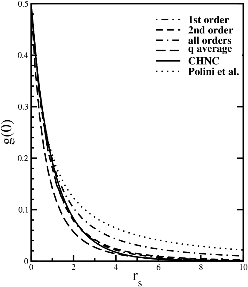
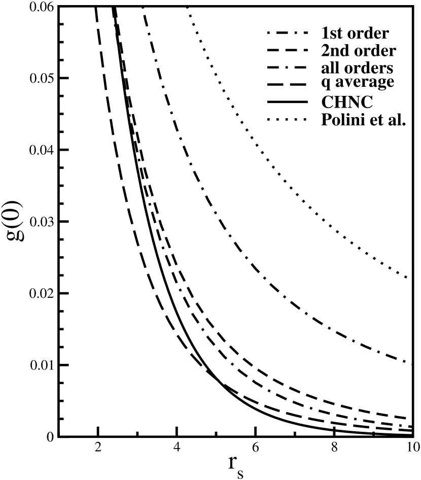
Figure 4: Two-particle distribution function at the origin as a function of $r_{s}$. Results of the analytical expansion to first order given by Eq. (21) (dot-dashed line), second order by Eq. (1) (dashed line), and infinite order [Eq. (22)] (dot-double-dashed line), and the average over the distribution of relative momentum [Eq. (23)] (long-dashed line) are displayed. The numerical results of Bulutay and Tanatar Bulu02 (solid line) and the interpolation results of Polini et al. Polini01 (dotted line) are also displayed. The right panel is a blow-up of the large $r_{s}$ region.

At zero distance, $g_{\uparrow\uparrow}(\rho=0)$ vanishes on account of the Pauli exclusion principle, while $g_{\uparrow\downarrow}(\rho=0)$ is determined by the $m=0$ component of the two-body wave function,

$$g_{\uparrow\downarrow}(\rho=0)=\langle|\Psi_{0}(\rho=0)|^{2}\rangle_{p_{\uparrow\downarrow}(k)}=\langle|\alpha_{0,0}|^{2}\rangle_{p_{\uparrow\downarrow}(k)}.$$ (18)

Since the distribution of the relative momentum of an electron pair is a smooth function, a good estimate of $\langle|\alpha_{0,0}|^{2}\rangle_{p_{\uparrow\downarrow}(k)}$ is obtained by making an expansion around the momentum where the distribution reach its maximum as:

$$\alpha_{0,0}\sim\frac{1}{G(r_{s})},$$ (19)

where the momentum dependence of $G$ have been dropped. Using the recurrent relation (12), we obtain a series expansion of $G(r_{s})$:

$$G(r_{s})=1+r_{s}\Big{\{}a_{1}+\sum_{m=1}^{\infty}\frac{{\cal A}(m)}{(2m+2)^{2}}\Big{\}}+$$

$$+r^{2}_{s}\Big{\{}a_{2}+\sum_{m=1}^{\infty}{\cal A}(m)\Big{[}\frac{1}{(2m+3)^{2}}\left(1+\frac{1}{(2m+2)^{2}}\right)+$$

$$+\left(\frac{1}{\pi}-\frac{3}{4}\right)\frac{1}{(2m+4)^{2}}\left(1+\frac{4}{(2m+2)^{2}}\right)+$$

$$+\sum_{n=1}^{\infty}{\cal A}(n)\frac{1}{(2n+2)^{2}(2n+2m+4)^{2}}\Big{]}\Big{\}}+O(r_{s}^{3})$$

$$\sim(1+0.6032~{}r_{s}+0.07263~{}r_{s}^{2})$$ (20)

where $\displaystyle a_{1}=\frac{1}{4}+\frac{1}{\pi}$ and $\displaystyle a_{2}=\frac{5}{9\pi}-\frac{1}{6}+\frac{1}{4}\left(\frac{1}{\pi}-\frac{3}{4}\right)^{2}$.

We can obtain $g(0)$ at any order in the expansion on the parameter $r_{s}$ since that $\displaystyle g(\rho=0)=\frac{1}{2}g_{\uparrow\downarrow}(0)=\frac{1}{2}\frac{1}{G(r_{s})^{2}}$. To first order in the expansion of $G(r_{s})$ the pair distribution is:

$$g(\rho=0)=\frac{1}{2}\frac{1}{[1+0.6032~{}r_{s}]^{2}}.$$ (21)

To second order we recover Eq. (1). Our approximation procedure also allows us to sum all the orders as:

$$g(\rho=0)=\frac{1}{2}\left(\sum_{n=0}^{\infty}\frac{\alpha_{0,n}}{\alpha_{0,0}}\right)^{-2}.$$ (22)

Finally, we also calculate $g(0)$ performing the average over the distribution of relative momenta:

$$g(0)=\frac{1}{2}g_{\uparrow\downarrow}(0)=\frac{1}{2}\int_{0}^{k_{F}}p(q)|\alpha_{0,0}(q,r_{s})|^{2}dq$$ (23)

where $\alpha_{0,0}(q,r_{s})$ is given by Eq. (15) and (16) and $p(q)$ by Eq. (17).

Fig. 4 displays the pair distribution function of a two-dimensional unpolarized electron gas at the origin as a function of the coupling-strength $r_{s}$. Results of the first order in the analytic expansion on $r_{s}$, Eq. (21), the second order, Eq. (1), and the infinite order solution, Eq. (22), together with the momentum average results, Eq. (23), are displayed. In addition, the results of the numerical calculation of Bulutay and Tanatar Bulu02 and the recent estimate by Polini et al.Polini01 are also included for comparison. Several conclusions can be gathered. By adding additional terms in the analytical expansion on $r_{s}$ we are able to closely approach the numerical resultsBulu02 in the low-density regime. Note that Eq. (1) is already a reliable analytical expression for $g(0)$. Fig. 4 also shows that the results of the momentum average approach, Eq. (23), are slightly below Bulutay and Tanatar results for small $r_{s}$, but become even closer to the numerical curve in the low-density regime. In this regime, the analytical expression obtained on Ref. Polini01, displays much larger values of $g(0)$ than the available numerical data.Tan89 ; Bulu02

The contact value of the pair distribution function changes when the electron gas is polarized. The spin polarization directly appears on the expression for $g(0)$, $\displaystyle g(0)=\frac{1-\zeta^{2}}{2}g_{\uparrow\downarrow}(0)$. In addition, the polarization modifies the distribution of momenta of the electron pair and, as consequence, the value of $g_{\uparrow\downarrow}(0)$. We calculate the spin resolved pair distribution function as:

$$g_{\uparrow\downarrow}(\zeta,\rho=0)=\int_{0}^{k_{+}}p_{\zeta}(q)|\alpha_{0,0}(q,r_{s})|^{2}dq.$$ (24)

where $p_{\zeta}(q)$ is the distribution of relative momentum in the polarized electron gas:

$$p_{\zeta}(q)=\frac{8q}{\max(k^{2}_{F\uparrow},k^{2}_{F\downarrow})}\quad{\rm(for}\;0\leqslant q\leqslant k_{-})$$

$$p_{\zeta}(q)=\frac{8q}{\pi k^{2}_{F\uparrow}k^{2}_{F\downarrow}}\Big{[}k^{2}_{F\uparrow}\Big{(}\arccos(x)-x\sqrt{1-x^{2}}\Big{)}$$

$$+k^{2}_{F\downarrow}\Big{(}\arccos(y)-y\sqrt{1-y^{2}}\Big{)}\Big{]}$$

$$\hskip 72.26999pt{\rm(for}\;k_{-}\leqslant q\leqslant k_{+})$$ (25)

where $\displaystyle x=\Big{(}q+\frac{k^{2}_{F\uparrow}-k^{2}_{F\downarrow}}{4q}\Big{)}/k_{F\uparrow}$, $\displaystyle y=\Big{(}q-\frac{k^{2}_{F\uparrow}-k^{2}_{F\downarrow}}{4q}\Big{)}/k_{F\downarrow}$ and $k_{-}=|k_{F\uparrow}-k_{F\downarrow}|/2$, $k_{+}=(k_{F\uparrow}+k_{F\downarrow})/2$. The Fermi momentum for the spin up (down) population is related with the polarization and the Fermi momentum of the unpolarized gas ($k_{F}$) by $k_{F\uparrow}=k_{F}\sqrt{1+\zeta}$ and $k_{F\downarrow}=k_{F}\sqrt{1-\zeta}$.

Our results show that $g_{\uparrow\downarrow}(\zeta,\rho=0)$ is largely unaffected by the degree of spin polarization. The difference between $g_{\uparrow\downarrow}(\zeta=1,0)$ and its unpolarized counterpart $g_{\uparrow\downarrow}(\zeta=0,0)$ is, at most, a few percents for any given value of $r_{s}$. The absence of a significant dependence with the spin polarization was also found in previous calculations.Polini01 Moreover, given that the momentum dependence of our results is rather weak, we do not expect important changes if the free Fermi momentum distributions, Eq. (17) and (25), are replaced by the interacting ones.

IV Conclusions

We have calculated the pair distribution function in a two dimensional interacting electron gas, following an approach originally developed in three dimensions by Overhauser.Over95 Within this framework, the short range correlations of the Coulomb interaction are replaced by an effective potential, and the calculation of $g(\rho)$ is reduced to solving the corresponding two-electron scattering problem and averaging over the probability distribution of the momentum of the electron pair. Our results for $g(r)$ at moderate coupling strengths agree well with the numerical data.Tan89 At larger values of $r_{s}$, however, this approximation is unable to reproduce the strong quantum oscillations of the numerical results.

The analytic expression for $g(0)$ as a function of $r_{s}$, Eq. (1), derived in this context compares very favorably with the complete solution of the effective potential, Eq. (23), and with recent numerical calculations.Tan89 ; Bulu02 We believe that the discrepancy between the present results and the analytical expression obtained in Ref. Polini01, is essentially due to the different choice of effective potential (see Fig. 1). Besides, while we have used the same approach for all values of the electronic density and polarization, Polini et al. use an interpolating scheme between the results of a perturbative expansion at high-density and the Overhauser’s treatment of scattering processes in the low-density limit.

We have also studied the dependence of $g(0)$ with the spin polarization of the electron gas. We have found that the spin-up spin-down correlation function, $g_{\uparrow\downarrow}(0)$, is basically independent of the degree of polarization. Therefore, the polarization modifies $g(0)$ only through its dependence on the density, $\displaystyle g(0)=\frac{2n_{\uparrow}n_{\downarrow}}{n^{2}}g_{\uparrow\downarrow}(0)$.

Within this approach, further study of how the choice of the effective potential modifies the pair distribution function can provide valuable insight into the short range electronic correlations in real materials.

Acknowledgments

We are grateful to Dr. Bulutay and Dr. Tanatar for providing us with the results of their numerical calculation. We acknowledge the financial support provided by the Department of Energy, grant no. DE-FG02-01ER45897.

References

- (1) B. Davoudi, M. Polini, R. Asgari and M. P. Tosi, Phys. Rev. B 66, 075110 (2002).
- (2) F. Capurro, R. Asgari, M. Polini and M. P. Tosi, Z. Naturforsch. 57a, 237 (2002) and B. Davoudi, M. Polini, R. Asgari and M. P. Tosi, cond-mat/0206456.
- (3) P. Gori-Giorgi and J. P. Perdew, Phys. Rev. B 64, 155102 (2001) and cond-mat/0206147.
- (4) M. Polini, G. Sica, B. Davoudi and M. P. Tosi, J. Phys.: Condens. Matter 13, 3591 (2001).
- (5) J. P. Perdew, K. Burke and M. Ernzerhof, Phys. Rev. Lett. 77, 3865 (1996); 78, 1396 (1997).
- (6) E. Chacón and P. Tarazona, Phys. Rev. B 37, 4013 (1988).
- (7) O. Gunnarsson, M. Jonson and B.I. Lundqvist, Phys. Rev. B 20, 3136 (1979).
- (8) G. Niklasson, Phys. Rev. B 10, 3052 (1974).
- (9) X. Zhu and A. W. Overhauser, Phys. Rev. B 30, 3158 (1984).
- (10) D.L. Freeman, J. Phys. C 16, 711 (1983).
- (11) S. Nagano, K. S. Singwi and S. Ohnishi, Phys. Rev. B, 29, 1209 (1984).
- (12) B. Tanatar and D. M. Ceperley, Phys. Rev. Phys. B 39, 5005 (1989).
- (13) C. Bulutay and B. Tanatar, Phys. Rev. B 65, 195116 (2002).
- (14) A. W. Overhauser, Phys. Rev. B 3, 1888 (1971).
- (15) A. W. Overhauser, Can. J. Phys. 73, 683 (1995).
- (16) P. Ziesche, J. Tao, M. Seidl and J. P. Perdew, Int. J. Quantum Chem. 77, 819 (2000).
- (17) I. Nagy, Phys. Rev. B 60, 4404 (1999).
- (18) At large distances the two-electron wave function can be written as: .