Competitive Clustering in a Bi-disperse Granular Gas

Abstract

A bi-disperse granular gas in a compartmentalized system is experimentally found to cluster competitively: Depending on the shaking strength, the clustering can be directed either towards the compartment initially containing mainly small particles, or to the one containing mainly large particles. The experimental observations are quantitatively explained within a flux model.

Clustering is one of the important features of granular gases, arising from the inelastic collisions between the particles. Energy is dissipated in each collision such that a dense region will dissipate more energy, becoming even denser, resulting in the formation of a cluster of slow particles  Goldhirsch-Jaeger-Kadanoff . It is a prime example of structure formation in a system far from equilibrium.

Thus far, most attention has been given to clustering in mono-disperse systems where all particles are identical. In that case, the clustering simply occurs in a region that originally is a bit denser than the others. In the present paper we concentrate on a bi-disperse granular gas, consisting of large and small particles. Here the clustering turns out to be competitive: it can occur either in a region which originally is populated mainly by small particles, or in a region with mainly large particles.

The experimental setup (see Fig.1) consists of a cylindrical perspex tube with inner diameter 11.2 cm and height 42.2 cm, divided into two equal compartments by a wall of height 6.0 cm. This compartmentalizaton makes it possible to get a clear-cut picture of the clustering process. The tube is mounted on a shaker with adjustable amplitude $a$ and frequency $f$. The inverse shaking strength $D\propto 1/(af)^{2}$ (defined more precisely in Eq.(8) below) is one of the crucial parameters for the clustering behavior.

To minimize the effect of statistical fluctuations in the experiments, we take a sufficiently large number of beads of each species: $P_{1}=300$ large and $P_{2}=600$ small ones. The small and large beads are both made of steel (so they have the same coefficient of normal restitution, $e\approx 0.85$), with radius ratio $\psi\equiv r_{1}/r_{2}=2$.

Clustering behavior— The clustering behavior is strongly influenced by the initial distribution of the two species over the compartments. As an example we take an initial distribution in which compartment A has the majority of the large particles, and compartment B most of the small ones. This situation is depicted in Fig.1, left, with {$\frac{3}{5}P_{1},\frac{1}{3}P_{2}$} = {180, 200} in compartment A and {$\frac{2}{5}P_{1},\frac{2}{3}P_{2}$} = {120, 400} in compartment B. The outcome of the experiment (see Fig.1, right) depends on the shaking strength.

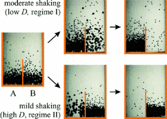
Figure 1: Images from two experiments with a mixture of $P_{1}$=300 large steel beads ($r_{1}=2.50$ mm, $m_{1}=0.500$ g) and $P_{2}$=600 smaller ones ($r_{2}=1.25$ mm, $m_{2}=0.063$ g). The initial distribution of the beads is the same in both experiments: {$\frac{3}{5}P_{1},\frac{1}{3}P_{2}$} in compartment A and {$\frac{2}{5}P_{1},\frac{2}{3}P_{2}$} in B. For moderate shaking strength ($f$ = 60.0 Hz, $a$ = 2.0 mm, top row) a cluster is formed in the compartment initially dominated by large particles (A). For milder shaking ($f$ = 37.5 Hz, $a$ = 2.0 mm, bottom row) the clustering takes place in the compartment initially containing most of the small particles (B).

The full bifurcation diagram is given in Fig.2: For sufficiently strong shaking (small $D$) a uniform distribution is found. This is denoted as regime 0. For moderate shaking strength (moderate $D$, regime I) the particles cluster in compartment A, the one initially dominated by large particles. The reason is as follows: Many of the small beads quickly cluster in compartment A, where the dissipation is highest due to the greater number of large beads, which (with their larger mass and surface area) act as “coolers”. The remaining beads in compartment B jump higher than before, since there are fewer collisions, and also large ones now start to make it over the wall into compartment A. After about twenty seconds to a minute (depending on the value of $D$) the final state is reached: a dynamical equilibrium with practically all large particles and most of the small ones in compartment A, and only a few rapid small particles in compartment B (see Fig.1, top row).

For very mild shaking (high $D$, regime II) the clustering process is much slower and, more importantly, it goes in the opposite direction. The particles now cluster in compartment B, i.e., in the compartment initially dominated by small particles (see Fig.1, bottom row). The series of events is as follows: First, the larger particles hardly jump at all. They stay close to the bottom, transferring energy from the vibrating bottom to the smaller particles, which thereby gain comparatively large velocities (like tennis balls jumping higher on top of a basketball than on the plain floor). So it is easier for the small beads to leave compartment A (with more large beads). The remaining particles become more mobile, and after a couple of minutes the first large beads start to make it across the wall into B, where they are immediately swallowed by the developing cluster. With every particle that leaves compartment A, the process progressively speeds up. The total clustering time is in the order of five to twenty minutes, steeply increasing with the value of $D$.

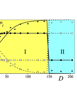
Figure 2: Bifurcation diagram showing the three different clustering regimes O, I, and II. The particle numbers $N_{i}$ ($i=1,2$) are given relative to the symmetric solution: $N_{i}-\frac{1}{2}P_{i}$. The squares and diamonds are experimental data, corresponding to the numbers of large and small particles respectively, in compartment A (solid) and B (open). The curves represent the equilibrium situation according to the theoretical flux model. The initial condition is always the same as in Fig.1.

Flux model — The above behavior can be explained in terms of a dynamical flux model. It is a generalization of the model derived by Eggers for clustering in the mono-disperse case  Eggers ; Weele-Meer01 ; Meer02 . First we consider the compartments separately, and from this derive the flux of particles leaving each compartment.

The gas within a compartment is assumed to be in thermal equilibrium with respect to the granular temperature $T={1\over 2}m_{i}\left<v_{i}^{2}\right>$ (the mean kinetic energy of the particles), which is taken to be the same for both species $i=1,2$. This is an approximation: Two different granular temperatures may in fact coexist in binary mixtures  Losert-Wildman-Feitosa (and at higher densities the species are known to segregate  Rosato-Knight-Hong ), but taking this into account would add an unknown and possibly not constant parameter to our model. As in ref. Eggers , and in fair agreement with molecular dynamics simulations  Mikkelsen-preprint , we assume that the granular temperature $T$ is approximately constant throughout the compartment.

The same simulations  Mikkelsen-preprint show that both species obey a barometric height distribution (as expected for dilute granular gases, where one can use the standard equation of state and momentum balance  Eggers ). That is, their number densities show an exponential decay with the height $z$:

$$n_{i}(z)=n_{i}(0)\exp(-m_{i}gz/T).$$ (1)

The density at ground level follows from $\Omega\int_{0}^{\infty}n_{i}(z)dz=N_{i}$ as $n_{i}(0)=m_{i}gN_{i}/\Omega T$. Here $N_{i}$ is the number of particles (of species $i$) in the compartment under consideration and $\Omega$ is its ground area. Eq.1 says that the larger particles, with larger $m_{i}$, become dilute faster with growing $z$ than the small particles.

The temperature $T$ is determined by the balance between energy input $J_{0}$ (through collisions with the bottom) and dissipation $Q$ (through the collisions between particles). To determine the energy input, we assume for simplicity a small-amplitude sawtooth motion of the bottom, such that colliding particles always find it moving upward with velocity $v_{b}=af$. This means that a particle coming down with vertical velocity component $v_{zi}$ is bounced back with $v_{zi}+2v_{b}$, and the energy gain per collision is $2m_{i}v_{b}(v_{zi}+v_{b})$. Multiplying this by the number of collisions ($\propto n_{i}(0)v_{zi}$ per species), and assuming an isotropic Maxwellian velocity distribution ($\left<v_{zi}^{2}\right>=\frac{1}{3}\left<v_{i}^{2}\right>$), this gives the rate of energy input:

$$J_{0}=\Omega\sum_{i=1,2}n_{i}(0)\left(\frac{4}{3}v_{b}T+\frac{2\sqrt{2}}{\sqrt{3}}v_{b}^{2}\sqrt{m_{i}T}\right).$$ (2)

As typically $v_{b}\ll v_{i}$, the first term is much larger than the second, which we therefore neglect. Then $J_{0}=\frac{4}{3}\Omega(n_{1}(0)+n_{2}(0))v_{b}T=\frac{4}{3}gv_{b}(m_{1}N_{1}+m_{2}N_{2})$.

This must be balanced by the rate of energy loss $Q$ through the inelastic collisions between the particles. It is equal to the product of the number of collisions per unit volume and the energy loss per collision ($\propto(1-e^{2})[m_{i}m_{j}/(m_{i}+m_{j})][v_{i}-v_{j}]^{2}$), averaged over the velocity distribution, and integrated over the whole compartment. It consists of three terms, representing collisions between two particles of type 1, type 2, and type 1 and 2, respectively  note1 :

$$Q = \frac{16\sqrt{\pi}g}{\Omega}(1-e^{2})T^{3/2}\times$$

$$\hskip-14.22636pt\left(r_{1}^{2}\sqrt{m_{1}}N_{1}^{2}+r_{2}^{2}\sqrt{m_{2}}N_{2}^{2}+\frac{4}{7}(r_{1}+r_{2})^{2}\sqrt{m_{12}}N_{1}N_{2}\right),$$

with

$$\sqrt{m_{12}}=\frac{m_{1}m_{2}\left(\frac{m_{1}}{\sqrt{m_{2}}}+\frac{m_{2}}{\sqrt{m_{1}}}+\frac{3}{4}(\sqrt{m_{1}}+\sqrt{m_{2}})\right)}{(m_{1}+m_{2})^{2}}.$$ (4)

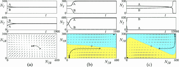
Figure 3: Evolution of the bi-diperse system, calculated from the flux model, for (a) $D=1$, (b) $D=100$, and (c) $D=200$. The top rows show the number of large and small particles as a function of time (note the different time scales): the solid curves represent compartment A, the dashed ones compartment B. The flow diagrams (bottom row) show how the contents of B evolve: $N_{1B}$ (large) and $N_{2B}$ (small). The cross indicates the initial condition {$N_{1B},N_{2B}$}={$120,400$}. The transition from (a) to (b) comes about through a bifurcation, whereas the transition from (b) to (c) is seen to be the result of a shifting basin boundary.

Equating $J_{0}$ and $Q$ yields the granular temperature $T$ of the compartment:

$$T=\frac{(af)^{2}\mu}{144\pi(1-e^{2})^{2}},$$ (5)

where the effective mass $\mu$ is given by:

$$\mu(N_{1},N_{2}) =$$

$$\hskip-48.36958pt\left(\frac{\Omega(m_{1}N_{1}+m_{2}N_{2})}{r_{1}^{2}\sqrt{m_{1}}N_{1}^{2}+r_{2}^{2}\sqrt{m_{2}}N_{2}^{2}+\frac{4}{7}(r_{1}+r_{2})^{2}\sqrt{m_{12}}N_{1}N_{2}}\right)^{2}.$$

It is through this quantity that the populations of the two species within one compartment influence each other.

The central quantity of the model is the flux function $F_{i}$, i.e., the number of particles (of species $i$) that leave the compartment per unit time. It is the product of the density $n_{i}(z)$ and the horizontal velocity (= $\sqrt{2T/3m_{i}}$), integrated over the space above the wall (width $b$) from $z=h$ to some cut-off height $h+H$ note2 :

$$F_{i}(N_{1},N_{2}) =\sqrt{\frac{2T}{3m_{i}}}b\int_{h}^{H}n_{i}(z)dz$$ (7)

$$=\sqrt{\frac{2T}{3m_{i}}}\frac{bN_{i}}{\Omega}e^{-m_{i}gh/T}\left(1-e^{-m_{i}gH/T}\right)$$

$$=AN_{i}\sqrt{\frac{m_{i}}{\mu}}e^{-Dm_{i}/\mu}.$$

In the last step we have linearized exp$(-m_{i}gH/T)$, implying that $H\ll\left<v_{i}^{2}\right>/g$. The prefactor determining the absolute rate of the flux is given by $A=12\sqrt{2\pi/3}(1-e^{2})gbH/\Omega af$. The dimensionless parameter $D$, which governs the clustering behavior, has the form

$$D=144\pi\frac{gh}{(af)^{2}}(1-e^{2})^{2}.$$ (8)

The evolution of the number of particles $N_{iA}$ in compartment A ($i=1,2$) is given by the net balance between the (outgoing) flux from A to B and the (incoming) flux from B to A:

$$\frac{dN_{iA}}{dt} =-F_{i}(N_{1A},N_{2A})+F_{i}(N_{1B},N_{2B})$$ (9)

$$=-F_{i}(N_{1A},N_{2A})+F_{i}(P_{1}-N_{1A},P_{2}-N_{2A}),$$

where we have used particle conservation, $N_{iA}+N_{iB}=P_{i}$. The evolution of the (complementary) particle numbers in compartment B is governed by the same equation with A and B interchanged.

Flux model vs. experiment — In Fig.2 the results from the flux model are shown together with the experimental data, using the same initial distribution as in Fig.1. The agreement between theory and experiment is very good, and the same three regimes are found: For vigorous shaking (regime 0, $D<10$) the system settles into the unclustered homogeneous state. For moderate shaking (regime I, $10<D<150$) we find clustering in compartment A, and for mild shaking ($D>150$) the clustering takes place in compartment B. The transition from regime I to II is quite abrupt.

The experimental observation that the small particles always (in both regimes I and II) are the first to cluster, followed later by the large ones, is also reflected in the flux model. This can be seen in Fig.3, where the evolution of the various particle numbers (obtained from Eq.9) is shown. The same plots also illustrate the different timescales for type-I and type-II clustering: The time it takes the system to reach its equilibrium situation grows rapidly with growing $D$ (decreasing shaking strength), just as in experiment.

In the lower part of Fig.3 the corresponding flow diagrams are depicted, showing how the particle numbers $N_{1B}$ and $N_{2B}$ in compartment B evolve, for any initial condition. The cross denotes the initial condition used in the experiments ({$N_{1B},N_{2B}$}={$120,400$}), and the arrows show the evolution of the system. For very strong shaking (left plot) only one stable fixed point exists: the uniform distribution {150,300}.

In the middle plot, for moderate shaking strength, the homogeneous state has become unstable and has given way to two new stable fixed points. These correspond to the compartment B being either nearly empty (fixed point in the lower left corner) or well-filled (upper right). Their basins of attraction are indicated by the shading. Our starting point happens to lie in the basin of the lower left point, and so we end up with compartment B being nearly empty. The arrows show that the small particles cluster first, and only when these have attained their final distribution do the large ones follow. Indeed, the flux of large particles is only appreciable when the number of small particles in the compartment has become very low.

Finally, in the rightmost plot (for mild shaking) we see that the basin boundary has shifted, which explains the switch from regime I to regime II: Our initial condition now lies within the basin of attraction of the fixed point in the upper right corner. So we end up with a full compartment B. The same plot shows that the fixed points move further into their corners as $D$ grows, i.e., the clustering becomes more pronounced for decreasing shaking strength, just as in the mono-disperse case  Eggers ; Weele-Meer01 .

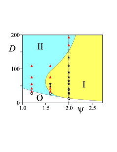
Figure 4: Phase diagram, showing the three clustering regimes as a function of the inverse shaking strength $D$ and the size ratio $\psi=r_{1}/r_{2}$. The shaded areas are calculated from the flux model, and the open circles (no clustering), stars (type I clustering), and triangles (type II clustering) correspond to experiments. The experimental results on the vertical dashed line $\psi=2$ also feature in Fig.2. The initial distribution of particles is always taken to be the same as in Figs. 1-3.

Further parameters — Until now we have taken the ratio of the radii $\psi=r_{1}/r_{2}=2$, but how does the phenomenon depend on $\psi$ in general? This ratio has a marked effect on the critical $D$-values where the transitions between the regimes 0, I, and II take place. In Fig.4 we show the position of these regimes as a function of $\psi$, from the flux model and from experiments. The vertical dashed line corresponds to $\psi=2$ studied in Figs. 1-3. It is seen that for $\psi<1.5$ the transition to regime II is immediate: here the larger beads are not sufficiently big to compensate for the fact that they are a minority. It is the larger number of beads that decide where the cluster goes, just as for the mono-disperse case ($\psi=1$). On the other hand, for high values of $\psi$, the dominant size of the large beads always makes them the decisive factor (only regime I survives). It is precisely the intermediate region $1.5<\psi\lesssim 2.3$ in which the competition takes place. For $\psi\approx 1.6$ we witness the particularly interesting sequence 0-II-I-II, both in the model and in experiment.

Another parameter of interest is the ratio between the total particle numbers of each species, $\sigma\equiv P_{1}/P_{2}$ (up to now we have always taken $\sigma=1/2$). Also this ratio obviously has a big influence on the clustering behavior: a larger value of $\sigma$ means that the large beads become a more important minority (or even a majority for $\sigma>1$) and hence type-I clustering will gain ground.

Conclusion — The clustering behavior of a bi-disperse granular gas is much richer than the mono-disperse case, and shows a surprising new feature: The clustering can be directed either towards the compartment initially containing mainly large particles (type-I clustering) or to the one containing mainly small particles (type-II), simply by adjusting the shaking strength. All the experimental observations can be explained quantitatively by a bi-disperse extension of the Eggers flux model.

Acknowledgments: This work is part of the research program of the Stichting FOM, which is financially supported by NWO.

References

- (1) I. Goldhirsch and G. Zanetti, Phys. Rev. Lett. 70, 1619 (1993); H. Jaeger, S. Nagel, and R. Behringer, Rev. Mod. Phys. 68, 1259 (1996); L. Kadanoff, Rev. Mod. Phys. 71, 435 (1999).
- (2) J. Eggers, Phys. Rev. Lett. 83, 5322 (1999).
- (3) K. van der Weele, D. van der Meer, M. Versluis, and D. Lohse, Europhys. Lett. 53, 328 (2001); D. van der Meer, K. van der Weele, and D. Lohse, Phys. Rev. E 63 061304 (2001).
- (4) D. van der Meer, K. van der Weele, and D. Lohse, Phys. Rev. Lett. 88, 174302 (2002).
- (5) W. Losert, D.G.W. Cooper, J. Delour, A. Kudrolli, and J.P. Gollub, Chaos 9, 682 (1999); R.D. Wildman and D.J. Parker, Phys. Rev. Lett. 88, 064301 (2002); K. Feitosa and N. Menon, Phys. Rev. Lett. 88, 198301 (2002).
- (6) A. Rosato, K.J. Strandburg, F. Prinz, and R.H. Swendsen, Phys. Rev. Lett. 58, 1038 (1987); J.B. Knight, H.M. Jaeger, and S.R. Nagel, Phys. Rev. Lett. 70, 3728 (1993); D.C. Hong, P.V. Quinn, and S. Luding, Phys. Rev. Lett. 86, 3423 (2001).
- (7) R. Mikkelsen et al., preprint (University of Twente, 2002).
- (8) We neglect the dissipation resulting from collisions with the wall, treating them as being completely elastic.
- (9) Above the cut-off height, the state variables of the two compartments are in equilibrium and hence no net flux occurs. In principle, will depend on the mean free path of the particles, but here we take it to be constant. Naively integrating up to would lead to an (unphysical) non-zero flux for . To see this, consider a compartment without any type 2 particles: then (from Eqs. 5 and Competitive Clustering in a Bi-disperse Granular Gas) and hence loses its dependence in the dilute limit (cf. second line of Eq. 7), making it non-zero for .