Andreev Reflection in Ferromagnet/Superconductor/Ferromagnet Double Junction Systems

Abstract

We present a theory of Andreev reflection in a ferromagnet/superconductor/ferromagnet double junction system. The spin polarized quasiparticles penetrate to the superconductor in the range of penetration depth from the interface by the Andreev reflection. When the thickness of the superconductor is comparable to or smaller than the penetration depth, the spin polarized quasiparticles pass through the superconductor and therefore the electric current depends on the relative orientation of magnetizations of the ferromagnets. The dependences of the magnetoresistance on the thickness of the superconductor, temperature, the exchange field of the ferromagnets and the height of the interfacial barriers are analyzed. Our theory explains recent experimental results well.

I Introduction

The spin-dependent transport through magnetic nanostructures has attracted much interest.maekawaBOOK In the early 1970s, Meservey and Tedrow have showed that tunneling electrons between a ferromagnetic metal (Fe, Co, Ni) and a thin film of superconducting aluminium (Al) are spin-polarized.meservey The ferromagnet/insulator/superconductor (FM/I/SC) tunnel junctions are one of the most powerful tools to extract the spin polarization of the conduction electrons near the Fermi level. In FM/I/SC and FM/I/SC/I/FM tunnel junctions, the suppression of superconducting gap due to spin accumulation by injection of spin polarized quasiparticles (QP’s) has been shown.vasko ; dong ; yeh ; liu ; chen ; takahashiPRL The QP’s spin transport and relaxation in SC has been studied in detail. yamashita ; takahashiJMMM ; takahashiHOLL

In recent years, much attention has been focused on FM/SC metallic contacts both theoreticallyde_jong ; kikuchi ; hima ; zhu ; igor ; kashiwaya and experimentally soulen ; soulen2 ; ji ; strijkers ; shashi since the spin polarization of conduction electrons is measured by using the Andreev reflectionandreev : An electron injected from the FM into the SC is reflected as a hole at the FM/SC interface and a Cooper pair is generated in the SC. The Andreev reflection includes a conversion process of the QP current to the supercurrent carried by Cooper pairs in the range of the penetration depth, which is approximately equal to the Ginzburg-Landau (GL) coherence length,GL from the FM/SC interface.BTK Thus, a FM/SC/FM double junction is particularly interesting because the magnetoresistance is expected due to the overlap of the QP penetration in the SC by the Andreev reflection. Recently, Gu et al. have measured the magnetoresistance in a current perpendicular to plane (CPP) geometry consisting of a superconducting niobium (Nb) thin film sandwiched by ferromagnetic permalloys (Py) and proposed a method for estimating the penetration depth by measuring the magnetoresistance.gu

In this paper, we present a theory of the Andreev reflection in the FM/SC/FM double junction system and derive an expression of the current through the junction by extending the theory of Blonder, Tinkham and Klapwijk (BTK).BTK We numerically calculate the current for the parallel and anti-parallel alignments of magnetizations, and investigate the dependences of the magnetoresistance on the thickness of the SC, temperature, the exchange field of FM’s and the height of the interfacial barriers. It is shown that these dependences are understood by considering the penetration of quasiparticles to the SC by the Andreev reflection process. Finally, we compare our results with the recent experimental results by Gu et al..gu

II Model and Formulation

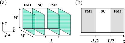
Figure 1: (a) Schematic diagram of a ferromagnet/superconductor/ferromagnet (FM1/SC/FM2) double junction system. A superconductor with a thickness of $L$ is sandwiched by two semi-infinite ferromagnetic electrodes. The system is rectangular and the cross section is a square of side $W$. (b) The current flows along the $z$-axis. The interfaces between FM1/SC and SC/FM2 are located at $z=-L/2$ and $z=L/2$, respectively.

We consider a FM1/SC/FM2 double junction system consisting of three rectangular blocks as shown in Figs. 1(a) and 1(b). The cross section of the system is a square of side $W$ and the thickness of the SC is $L$. The current flows along the $z$-axis and the interfaces between FM1/SC and SC/FM2 are located at $z=-L/2$ and $z=L/2$, respectively. For simplicity, we assume that the system is symmetric: FM1 and FM2 are made of the same ferromagnetic materials and the potentials for the left and right interfaces are the same. The system we consider is described by the following Bogoliubov-de Gennes (BdG) equation BdG :

$$\left({\begin{array}[]{*{20}c}\!\!{H_{0}\!-\!h_{ex}(z)\sigma}&\Delta(z)\\ {\Delta^{*}(z)}&{-{H_{0}\!-\!h_{ex}(z)\sigma}}\\ \end{array}}\!\!\right)\!\!\left(\!\!{\begin{array}[]{*{20}c}{f_{\sigma}\left({{\bf r}}\right)}\\ {g_{\sigma}\left({{\bf r}}\right)}\\ \end{array}}\!\!\right)\!=\!E\!\left(\!\!{\begin{array}[]{*{20}c}{f_{\sigma}\left({{\bf r}}\right)}\\ {g_{\sigma}\left({{\bf r}}\right)}\\ \end{array}}\!\!\right),$$ (7)

where $H_{0}\equiv-({\hbar}^{2}/2m){\nabla}^{2}-\mu_{F}$ is the single particle Hamiltonian, $E$ is the QP energy measured from the Fermi energy $\mu_{F}$ and $\sigma=+(-)$ is for the up-(down-)spin band. The exchange field $h_{ex}\left(z\right)$ is given by

$$h_{ex}\left(z\right)=\left\{\begin{array}[]{ll}h_{0}&(z<-L/2)\\ 0&(-L/2<z<L/2)\\ \pm h_{0}&(L/2<z)\end{array}\right.,$$ (8)

where $+h_{0}$ and $-h_{0}$ represent the exchange fields for the parallel and anti-parallel alignments, respectively. The superconducting gap is expressed as

$$\Delta\left(z\right)=\left\{{\begin{array}[]{cl}0&(z<-L/2,L/2<z)\\ \Delta&(-L/2<z<L/2)\end{array}}\right..$$ (9)

We assume that the temperature dependence of the superconducting gap is given by $\Delta=\Delta_{0}\tanh{\left(1.74\sqrt{{T_{c}}/{T}-1}\right)}$,belzig where $\Delta_{0}$ is the superconducting gap at $T=0$ and $T_{c}$ is the superconducting critical temperature. In order to capture the essential effect of the interfacial scattering, we employ the following $\delta$-function type potential at the interfaces:

$$H\left(z\right)=\frac{\hbar^{2}k_{F}}{m}Z\left\{\delta\left(z+L/2\right)+\delta\left({z-L/2}\right)\right\}.$$ (10)

Throughout this paper, we neglect the spin-flip scattering in the SC and the proximity effect near the interfaces.strijkers

Since the system is rectangular, the wave function in the transverse ($x$ and $y$) directions is given by

$${\rm S}_{nl}(x,y)\equiv\sin{\left(n\pi x/W\right)}\sin{\left(l\pi y/W\right)},$$ (11)

where $n$ and $l$ are the quantum numbers which define the channel. The eigenvalue of the transverse mode for the channel ($n$,$l$) is

$$E_{nl}=\frac{\hbar^{2}}{2m}\left[{{\left(\frac{n\pi}{W}\right)}^{2}+{\left(\frac{l\pi}{W}\right)}^{2}}\right].$$ (12)

The solution of the BdG equation (7) in the SC region is given by

$$\begin{array}[]{l}\Psi_{\pm k_{nl}^{+}}({\bf r})=\left(\begin{array}[]{c}\!\!\mbox{$u_{0}$}\!\!\\ \!\!\mbox{$v_{0}$}\!\!\end{array}\right)e^{\pm ik_{nl}^{+}z}\,{\rm S}_{nl}(x,y),\\ \Psi_{\pm k_{nl}^{-}}({\bf r})=\left(\begin{array}[]{c}\!\!\mbox{$v_{0}$}\!\!\\ \!\!\mbox{$u_{0}$}\!\!\end{array}\right)e^{\pm ik_{nl}^{-}z}\,{\rm S}_{nl}(x,y),\end{array}$$ (19)

where $u_{0}$ and $v_{0}$ are the coherence factors expressed as

$$u_{0}^{2}=1-v_{0}^{2}=\frac{1}{2}\left[{1+\frac{{\sqrt{E^{2}-\Delta^{2}}}}{E}}\right],$$ (20)

and $k_{nl}^{+(-)}$ is the $z$ component of the wave number of an electron-(hole-)like QP in the channel $(n,l)$ defined as

$$k_{nl}^{\pm}=\frac{\sqrt{2m}}{\hbar}\sqrt{\mu_{F}\pm\sqrt{E^{2}-\Delta^{2}}-E_{nl}}.$$ (21)

In the FM region, the solutions are given by

$$\begin{array}[]{l}\Psi_{\pm p_{\sigma,nl}^{+}}({\bf r})=\left(\begin{array}[]{c}\!\!\mbox{$1$}\!\!\\ \!\!\mbox{$0$}\!\!\end{array}\right)e^{\pm ip_{\sigma,nl}^{+}z}\,{\rm S}_{nl}(x,y),\\ \Psi_{\pm p_{\sigma,nl}^{-}}({\bf r})=\left(\begin{array}[]{c}\!\!\mbox{$0$}\!\!\\ \!\!\mbox{$1$}\!\!\end{array}\right)e^{\pm ip_{\sigma,nl}^{-}z}\,{\rm S}_{nl}(x,y),\end{array}$$ (28)

where $p_{\sigma,nl}^{+(-)}$ is the $z$ component of the wave number of an electron (hole) with $\sigma$-spin in the channel $(n,l)$;

$$p_{\sigma,nl}^{\pm}=\frac{\sqrt{2m}}{\hbar}\sqrt{\mu_{F}\pm E\pm\sigma h_{ex}-E_{nl}}.$$ (29)

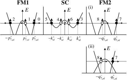
Figure 2: Schematic diagrams of energy vs. momentum for the FM1/SC/FM2 double junction system with the parallel and anti-parallel alignments of the magnetizations are shown in panels (i) and (ii), respectively. The open circles denote holes, the closed circles electrons, and the arrows point in the direction of the group velocity. The incident electron with up-spin in the channel ($n,l$) is denoted by 0, along with the resulting scattering processes: the Andreev reflection (1), the normal reflection (2) at the interface of FM1/SC, the transmission to the SC (3, 4) and the reflection at the interface of SC/FM2 (5, 6), the transmission as an electron to the FM2 (7) and the one as a hole (8).

The wave function of the FM1/SC/FM2 double junction system is given by the linear combination of the solutions. Let us consider the scattering of an electron with up-spin in the channel $(n,l)$ injected into the SC from the FM1 (0 in Fig.2). There are the following eight processes: the Andreev reflection (1 in Fig.2), the normal reflection (2 in Fig.2) at the interface of FM1/SC, the transmission to the SC (3, 4 in Fig.2) and the reflection at the interface of SC/FM2 (5, 6 in Fig.2), the transmission as an electron to the FM2 (7 in Fig.2) and the one as a hole (8 in Fig.2). Therefore, the wave function in the FM1 $(z<-L/2)$ is given by

$$\Psi^{\rm FM1}_{\sigma,nl}({\bf r}) = \Bigg{[}\left(\begin{array}[]{c}\!\!\mbox{$1$}\!\!\\ \!\!\mbox{$0$}\!\!\end{array}\right)e^{ip_{\sigma,nl}^{+}\left(z+\frac{L}{2}\right)}+a_{\sigma,nl}\left(\begin{array}[]{c}\!\!\mbox{$0$}\!\!\\ \!\!\mbox{$1$}\!\!\end{array}\right)e^{ip_{\sigma,nl}^{-}\left(z+\frac{L}{2}\right)}$$ (34)

$$+ b_{\sigma,nl}\left(\begin{array}[]{c}\!\!\mbox{$1$}\!\!\\ \!\!\mbox{$0$}\!\!\end{array}\right)e^{-ip_{\sigma,nl}^{+}\left(z+\frac{L}{2}\right)}\Bigg{]}{\rm S}_{nl}(x,y).$$ (37)

In the SC $(-L/2<z<L/2)$ we have

$$\Psi^{\rm SC}_{\sigma,nl}({\bf r})=\Bigg{[}\alpha_{\sigma,nl}\left(\begin{array}[]{c}\!\!\mbox{$u_{0}$}\!\!\\ \!\!\mbox{$v_{0}$}\!\!\end{array}\right)e^{ik_{nl}^{+}\left(z+\frac{L}{2}\right)}$$ (40)

$$+\beta_{\sigma,nl}\left(\begin{array}[]{c}\!\!\mbox{$v_{0}$}\!\!\\ \!\!\mbox{$u_{0}$}\!\!\end{array}\right)e^{-ik_{nl}^{-}\left(z+\frac{L}{2}\right)}+\xi_{\sigma,nl}\left(\begin{array}[]{c}\!\!\mbox{$u_{0}$}\!\!\\ \!\!\mbox{$v_{0}$}\!\!\end{array}\right)e^{-ik_{nl}^{+}\left(z-\frac{L}{2}\right)}$$ (45)

$$+\eta_{\sigma,nl}\left(\begin{array}[]{c}\!\!\mbox{$v_{0}$}\!\!\\ \!\!\mbox{$u_{0}$}\!\!\end{array}\right)e^{ik_{nl}^{-}\left(z-\frac{L}{2}\right)}\Bigg{]}{\rm S}_{nl}(x,y),$$ (48)

and in the FM2 $(L/2<z)$

$$\begin{split}\Psi^{\rm FM2}_{\sigma,nl}({\bf r})&=\Bigg{[}c_{\sigma,nl}\left(\begin{array}[]{c}\!\!\mbox{$1$}\!\!\\ \!\!\mbox{$0$}\!\!\end{array}\right)e^{iq_{\sigma,nl}^{+}\left(z-\frac{L}{2}\right)}\\ &+d_{\sigma,nl}\left(\begin{array}[]{c}\!\!\mbox{$0$}\!\!\\ \!\!\mbox{$1$}\!\!\end{array}\right)e^{-iq_{\sigma,nl}^{-}\left(z-\frac{L}{2}\right)}\Bigg{]}{\rm S}_{nl}(x,y).\end{split}$$ (49)

Here $p_{\sigma,nl}^{\pm}$, $k_{nl}^{\pm}$ and $q_{\sigma,nl}^{\pm}$ are the wave numbers in the FM1, SC and FM2, respectively. The coefficients $a_{\sigma,nl},b_{\sigma,nl},c_{\sigma,nl},d_{\sigma,nl},\alpha_{\sigma,nl},\beta_{\sigma,nl}$, $\xi_{\sigma,nl}$, and $\eta_{\sigma,nl}$ are determined by matching the wave functions at the left and right interfaces. The matching conditions for the wave functions (37) - (49) at the interfaces are

$$\left\{\begin{split}&\Psi^{\rm FM1}_{\sigma,nl}\left(\mbox{$z=-\frac{L}{2}$}\right)=\Psi^{\rm SC}_{\sigma,nl}\left(\mbox{$z=-\frac{L}{2}$}\right),\\ &\Psi^{\rm SC}_{\sigma,nl}\left(\mbox{$z=\frac{L}{2}$}\right)=\Psi^{\rm FM2}_{\sigma,nl}\left(\mbox{$z=\frac{L}{2}$}\right),\\ &\frac{d\Psi^{\rm SC}_{\sigma,nl}}{{dz}}\Bigr{|}_{z=-\frac{L}{2}}\!\!-\frac{d\Psi^{\rm FM1}_{\sigma,nl}}{{dz}}\Bigr{|}_{z=-\frac{L}{2}}\!=\!\frac{{2mZ}}{{\hbar^{2}}}\Psi^{\rm FM1}_{\sigma,nl}\left(\mbox{$z=-\frac{L}{2}$}\right),\\ &\frac{d\Psi^{\rm FM2}_{\sigma,nl}}{{dz}}\Big{|}_{z=\frac{L}{2}}\!\!-\frac{d\Psi^{\rm SC}_{\sigma,nl}}{{dz}}\Big{|}_{z=\frac{L}{2}}\!=\!\frac{{2mZ}}{{\hbar^{2}}}\Psi^{\rm FM2}_{\sigma,nl}\left(\mbox{$z=\frac{L}{2}$}\right).\end{split}\right.$$ (50)

Solving Eq.(50), the probabilities of transmission and reflection are calculated following the BTK theory. BTK When an electron with $\sigma$-spin is injected from the FM1, the probability of the Andreev reflection $R_{\sigma,nl}^{he}$, the normal reflection $R_{\sigma,nl}^{ee}$ and the transmission as an electron and the one as a hole to the FM2, $T_{\sigma,nl}^{e^{\prime}e}$ and $T_{\sigma,nl}^{h^{\prime}e}$ are given by

$$\left\{\begin{split}&R_{\sigma,nl}^{he}\left(E\right)={\frac{p_{\sigma,nl}^{-}}{p_{\sigma,nl}^{+}}}\,a_{\sigma,nl}^{*}a_{\sigma,nl},\\ &R_{\sigma,nl}^{ee}\left(E\right)=b_{\sigma,nl}^{*}b_{\sigma,nl},\\ &T_{\sigma,nl}^{e^{\prime}e}\left(E\right)={\frac{q_{\sigma,nl}^{+}}{p_{\sigma,nl}^{+}}}\,c_{\sigma,nl}^{*}c_{\sigma,nl},\\ &T_{\sigma,nl}^{h^{\prime}e}\left(E\right)={\frac{q_{\sigma,nl}^{-}}{p_{\sigma,nl}^{+}}}\,d_{\sigma,nl}^{*}d_{\sigma,nl},\end{split}\right.$$ (51)

where the subscript $e^{\prime}(h^{\prime})$ in Eq. (51) indicates the electron (hole) in the FM2. Let us evaluate the current in the FM1. When the bias voltage $V$ is applied to the FM1/SC/FM2 system, the current carried by electrons with $\sigma$-spin is written as

$$I_{\sigma}^{e}=\frac{e}{h}\sum_{nl}\int_{0}^{\infty}{\left[{f_{\to}\left(E\right)-f_{\leftarrow}\left(E\right)}\right]}dE,$$ (52)

where $h$ is Planck constant and $f_{\to}\left(E\right)$ is the distribution function of an electron with a positive group velocity in the $z$ direction and expressed as

$$f_{\to}\left(E\right)=f_{0}\left(\mbox{$E-\frac{{eV}}{2}$}\right),$$ (53)

where $f_{0}\left(E\right)$ is the Fermi distribution function. The distribution function of the electron with a negative group velocity in the $z$ direction is written as

$$f_{\leftarrow}\left(E\right)$$

$$=R_{\sigma,nl}^{eh}f_{0}\left(\mbox{$E+\frac{eV}{2}$}\right)+R_{\sigma,nl}^{ee}f_{0}\left(\mbox{$E-\frac{eV}{2}$}\right)$$

$$\ \ \ +\frac{{v_{\sigma,nl}^{R}{\cal D}_{\sigma,nl}^{R}}}{{v_{\sigma,nl}^{L}{\cal D}_{\sigma,nl}^{L}}}\left[T_{\sigma,nl}^{ee^{\prime}}f_{0}\left(\mbox{$E+\frac{{eV}}{2}$}\right)+T_{\sigma,nl}^{eh^{\prime}}f_{0}\left(\mbox{$E-\frac{eV}{2}$}\right)\right]$$

$$=R_{\sigma,nl}^{eh}f_{0}{\left(\mbox{$E+\frac{eV}{2}$}\right)}+R_{\sigma,nl}^{ee}f_{0}\left(\mbox{$E-\frac{eV}{2}$}\right)$$

$$\ \ \ +T_{\sigma,nl}^{ee^{\prime}}f_{0}\left(\mbox{$E+\frac{{eV}}{2}$}\right)+T_{\sigma,nl}^{eh^{\prime}}f_{0}\left(\mbox{$E-\frac{eV}{2}$}\right),$$ (54)

where $v_{\sigma,nl}^{L(R)}$ is the Fermi velocity of an electron with $\sigma$-spin in the channel $(n,l)$ of the FM1 (FM2) and ${\cal D}_{\sigma,nl}^{L(R)}$ is the density of states of $\sigma$-spin band in the channel $(n,l)$ of the FM1 (FM2). Using the conservation of probability, $R_{\sigma,nl}^{eh}+R_{\sigma,nl}^{ee}+T_{\sigma,nl}^{ee^{\prime}}+T_{\sigma,nl}^{eh^{\prime}}=1$, we have

$$\begin{split}I_{\sigma}^{e}&=\frac{e}{h}\sum_{nl}\int_{0}^{\infty}\left({R_{nl,\sigma}^{eh}+T_{nl,\sigma}^{ee^{\prime}}}\right)\\ &\times\left[{f_{0}\left(\mbox{$E-\frac{eV}{2}$}\right)-f_{0}\left(\mbox{$E+\frac{eV}{2}$}\right)}\right]dE.\end{split}$$ (55)

The current carried by holes $I_{\sigma}^{h}$ is calculated in the similar way.

The total current in the FM1/SC/FM2 double junction system is obtained as

$$\begin{split}I&=\sum_{\sigma}\left[I_{\sigma}^{e}+I_{\sigma}^{h}\right]\\ &=\frac{e}{h}\sum_{nl,\sigma}\int_{0}^{\infty}\left(R_{nl,\sigma}^{eh}+R_{nl,\sigma}^{he}+T_{nl,\sigma}^{ee^{\prime}}+T_{nl,\sigma}^{hh^{\prime}}\right)\\ &\times\left[{f_{0}\left(\mbox{$E-\frac{eV}{2}$}\right)-f_{0}\left(\mbox{$E+\frac{eV}{2}$}\right)}\right]dE.\end{split}$$ (56)

Note that this expression of the current Eq. (56) reduces to the one derived by Lambertlambert for the normal metal/superconductor/normal metal system when $h_{0}=0$.

The magnetoresistance (MR) is defined as

$${\rm MR}\equiv\frac{R_{\rm AP}-R_{\rm P}}{R_{\rm P}},$$ (57)

where $R_{\rm P(AP)}=V/I_{\rm P(AP)}$ is the resistance in the parallel (anti-parallel) alignment.

III Results

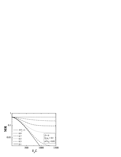
Figure 3: MR as a function of the thickness of the SC, $k_{F}L$. From top to bottom, temperature $T/T_{c}$ is 1, 0.9, 0.7, 0.5, 0.3, and 0.1. We assume $\xi_{Q}(E=T=0)=200/k_{F}$.

In Fig. 3 the MR is plotted as a function of the thickness of the SC, $L$, multiplied by the Fermi wave number $k_{F}$. We assume that the strength of the interfacial barrier $Z=0$ and the exchange field $h_{0}=0.5\mu_{F}$. The side length of the cross section is taken to be $W=1000/k_{F}$ throughout this paper. When the SC is in the normal conducting state ($T/T_{c}=1$), the MR is constant since we neglect the spin-flip scattering in the SC. When the SC is in the superconducting state ($T/T_{c}$ = 0.1, 0.3, 0.5, 0.7, and 0.9), the MR decreases with increasing the thickness of the SC. The MR at low temperatures $T/T_{c}\ll 1$ shows an exponential decrease in a wide range of $k_{F}L$. The decrease of the MR due to the superconductivity can be explained by considering the decay of the quasiparticle current in the SC. To obtain the charge and spin currents, we extend the BTK theory of the Andreev reflection BTK to the FM1/SC/FM2 double junction system.

Let us first consider the charge transport in the SC. When the current flows in the positive $z$ direction, electrons and holes are injected into the SC from the FM1 and the FM2, respectively. The conservation law of the charge density $Q_{\sigma}=e\sum_{nl}\left(|f_{nl}^{\sigma}|^{2}-|g_{nl}^{\sigma}|^{2}\right)$ in the SC, where $f_{nl}^{\sigma}$ and $g_{nl}^{\sigma}$ are electron- and hole-like components of the wave function in the channel ($n,l,\sigma$), respectively, is derived from the BdG equation (7) and obtained as

$$\frac{\partial Q_{\sigma}}{\partial t}+\nabla\cdot{\bf J}_{Q}^{\sigma}=\frac{4e\Delta}{\hbar}\sum_{nl}{\rm Im}({f_{nl}^{\sigma}}^{\ast}g_{nl}^{\sigma}),$$ (58)

where ${\bf J}_{Q}^{\sigma}$ is the QP current density with $\sigma$-spin and the $z$ component of ${\bf J}_{Q}^{\sigma}$ per unit area $j_{Q}^{\sigma}$ is written as

$$j_{Q}^{\sigma}(z) = \frac{e\hbar}{mW^{2}}\sum_{nl}\int_{0}^{W}\!\!\!\!dx\int_{0}^{W}\!\!\!\!dy\,\,$$ (59)

$$\times\,{\rm Im}\left({{f_{nl}^{\sigma}}}^{\ast}\frac{\partial}{\partial z}{f_{nl}^{\sigma}}+{{g_{nl}^{\sigma}}}^{\ast}\frac{\partial}{\partial z}{g_{nl}^{\sigma}}\right).$$

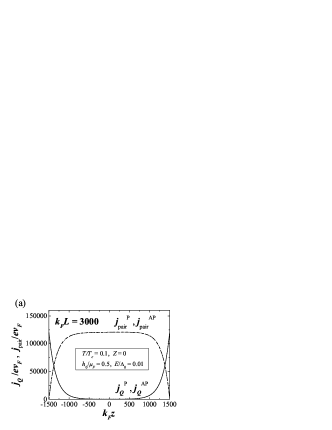
Figure 4: Spatial variation of the $z$ component of (a) the charge current density and (b) the spin current density in the SC with the thickness $L=3000/k_{F}$ is shown. $j_{Q}^{{\rm P(AP)}}$, $j_{\rm pair}^{{\rm P(AP)}}$ and $j_{\rm spin}^{{\rm P(AP)}}$ are the QP current density, the supercurrent density and the spin current density in the parallel (anti-parallel) alignment, respectively. We assume $\xi_{Q}(E=T=0)=200/k_{F}$.

The right hand side of Eq. (58) corresponds to the gradient of supercurrent carried by Cooper pair ${\bf J}_{\rm pair}^{\sigma}$ defined as

$$-\nabla\cdot{\bf J}_{\rm pair}^{\sigma}\equiv\frac{4e\Delta}{\hbar}\sum_{nl}{\rm Im}({f_{nl}^{\sigma}}^{\ast}g_{nl}^{\sigma}),$$ (60)

from which the $z$ component of ${\bf J}_{\rm pair}^{\sigma}$ per area $j_{\rm pair}^{\sigma}$ is obtained as

$$j_{\rm pair}^{\sigma}(z)=-\frac{4e\Delta}{\hbar W^{2}}\sum_{nl}\int_{0}^{W}\!\!\!\!dx\int_{0}^{W}\!\!\!\!dy$$

$$\times\,\int_{-L/2}^{z}\!\!\!\!dz^{\prime}\,\,{\rm Im}({{f_{nl}^{\sigma}}^{\ast}}{g_{nl}^{\sigma}}).$$ (61)

The $z$ coordinate dependences of the QP current density $j_{Q}=j_{Q}^{\uparrow}+j_{Q}^{\downarrow}$ and the supercurrent $j_{\rm pair}=j_{\rm pair}^{\uparrow}+j_{\rm pair}^{\downarrow}$ in the case that the thickness of the SC $L=3000/k_{F}$ are shown in Fig. 4(a).

Figure 5: The temperature dependence of the QP current penetration depth $\xi_{Q}$ for $E=0$. We assume $\xi_{Q}(E=T=0)=200/k_{F}$.

We find that $j_{Q}$ decays from the interfaces of the FM1/SC and the SC/FM2 and becomes zero in the interior of the SC. On the other hand, $j_{\rm pair}$ increases and becomes dominant in the interior of the SC to conserve the total current density. In the energy region below the superconducting gap ($E<\Delta$) where the energy of the transverse mode $E_{nl}$ is smaller than Fermi energy $\mu_{F}$, the wave number $k^{\pm}_{nl}$ is expanded as

$$\begin{split}k^{\pm}_{nl}&\sim\frac{\sqrt{2m}}{\hbar}{\left(\mu_{F}\pm i\sqrt{\Delta^{2}-E^{2}}\right)}^{\frac{1}{2}}\\ &\sim k_{F}\pm i\frac{1}{2\xi_{Q}}.\end{split}$$ (62)

The imaginary part in Eq. (62) gives the exponential decay term $\exp(-z/\xi_{Q})$ in $j_{Q}$, where $\xi_{Q}$ is the penetration depth given by

$$\xi_{Q}=\frac{\hbar v_{F}}{2\sqrt{\Delta^{2}-E^{2}}},$$ (63)

where $v_{F}$ is the Fermi velocity. $\xi_{Q}$ has a strong temperature dependence shown in Fig. 5. When the thickness of the SC is much larger than the penetration depth ($L\gg\xi_{Q}$) as in Fig. 4(a), $j_{Q}$ decays in the range of $\xi_{Q}$ from the interfaces. Note that $\xi_{Q}$ is approximately equal to the clean-limit GL coherence length $\xi(T)$ in the low energy regime: $\xi_{Q}(E=0)\sim 1.2\thinspace\xi(T)$.BTK

Next, we consider the spin transport in the SC. The conservation law of the spin density $S=P_{\uparrow}-P_{\downarrow}$, where $P_{\sigma}=\sum_{nl}({|f_{nl}^{\sigma}|}^{2}+{|g_{nl}^{\sigma}|}^{2})$, is derived from the BdG equation (7) and expressed as

$$\frac{\partial S}{\partial t}+\nabla\cdot{\bf J}_{\rm spin}=0,$$ (64)

where ${\bf J}_{\rm spin}={\bf J}_{P}^{\uparrow}-{\bf J}_{P}^{\downarrow}$ is the spin current density. The $z$ component of ${\bf J}_{P}^{\sigma}$ per unit area $j_{P}^{\sigma}$ is written as

$$j_{P}^{\sigma}(z) = \frac{\hbar}{mW^{2}}\sum_{nl}\int_{0}^{W}\!\!\!\!dx\int_{0}^{W}\!\!\!\!dy\,\,$$ (65)

$$\times\,{\rm Im}\left({{f_{nl}^{\sigma}}}^{\ast}\frac{\partial}{\partial z}{f_{nl}^{\sigma}}-{{g_{nl}^{\sigma}}}^{\ast}\frac{\partial}{\partial z}{g_{nl}^{\sigma}}\right).$$

Figure 4(b) shows the $z$ coordinate dependence of the spin current density $j_{\rm spin}=j_{P}^{\uparrow}-j_{P}^{\downarrow}$ in the SC with the thickness $L=3000/k_{F}$. As shown in Fig. 4(b), no spin current flows through the SC both in the parallel and in the anti-parallel alignments because the QP current with spin changes to the supercurrent carried by Cooper pairs with no spin. This means that the spin injected from FM1 does not reach to the FM2. As a result, the QP current density in the parallel alignment $j_{Q}^{\rm P}$ and that in the anti-parallel alignment $j_{Q}^{\rm AP}$ are almost the same as shown in Fig. 4(a).

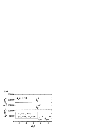
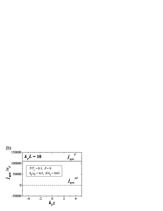
Figure 6: Spatial variation of the $z$ component of (a) the charge current density and (b) the spin current density in the SC with the thickness $L=10/k_{F}$ is shown. The parameters are the same as in Fig. 4.

The $z$ coordinate dependence of the charge current in the case that the thickness of the SC is much smaller than the penetration depth ($L\ll\xi_{Q}$) is shown in Fig. 6(a), where the QP current density $j_{Q}$ is almost constant and the supercurrent density $j_{\rm pair}$ is nearly zero in the SC. As shown in Fig. 6(b), the value of the spin current in the parallel alignment is larger than that in the anti-parallel alignment because the value of QP current with up-spin is much larger than that with down-spin in the parallel alignment, whereas the value of QP current with up-spin is equal to that with down-spin in the anti-parallel alignment. This means that the spin injected from the FM1 is transferred to the FM2 and therefore the value of the QP current density strongly depends on the relative orientation of the FM’s magnetizations shown in Fig. 6(a).

From the above discussion, the result shown in Fig. 3 is understood as follows. In the SC, the QP current with spin decreases exponentially and changes to the supercurrent carried by Cooper pairs with no spin in the range of $\xi_{Q}$ from the interfaces. As a result, it becomes difficult to transfer the spin from the FM1 to the FM2 and the MR decreases with increasing the thickness of the SC. The finite MR in the region of large $L$ is due to the QP’s with energy above the superconducting gap ($E>\Delta$).

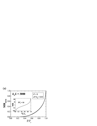
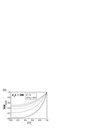
Figure 7: MR normalized by the value at $T_{c}$ (${\rm MR_{norm}}$) is plotted as a function of temperature. The thickness of the SC is taken to be $k_{F}L=3000$ and 300 in panels (a) and (b), respectively. From bottom to top, the exchange field $h_{0}/\mu_{F}$ = 0.1, 0.3, 0.5, 0.7, and 0.9. The MR at $T=T_{c}$ is plotted as a function of the exchange field $h_{0}$ in the inset of panel (a). We assume $\xi_{Q}(E=T=0)=200/k_{F}$.

The temperature dependences of the MR normalized by the value at $T_{c}$ (${\rm MR_{norm}}$) for several values of the exchange field $h_{0}$ in the case of $L=3000/k_{F}$ and $L=300/k_{F}$ are shown in Figs. 7(a) and 7(b), respectively. The ${\rm MR_{norm}}$ decreases with decreasing temperature because the number of electrons and holes with the energy $E>\Delta$ which contribute to the ${\rm MR_{norm}}$ decreases with decreasing temperature. At low temperatures, electrons and holes mainly distribute in the energy region $E<\Delta$. When the thickness of the SC is much larger than the penetration depth (Fig. 7(a)), electrons and holes with energy $E<\Delta$ injected to the SC do not contribute to the ${\rm MR_{norm}}$ because the QP current changes to the supercurrent in the SC by the Andreev reflection and the QP transmission from the FM1 to the FM2 does not occur. As a result, the ${\rm MR_{norm}}$ becomes zero at low temperatures $T/T_{c}\lesssim 0.4$. On the other hand, when the thickness of the SC is comparable to the penetration depth (Fig. 7(b)), the QP transmission by the Andreev reflection in the energy region $E<\Delta$ occurs and therefore the finite ${\rm MR_{norm}}$ remains even at low temperatures.

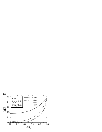
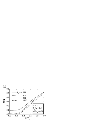
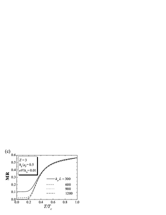
Figure 8: MR for the system with a several value of interfacial barrier is plotted as a function of temperature $T/T_{c}$. The strength of the interfacial barrier is $Z=0$, $1$ and $3$ for panels (a), (b) and (c) respectively. From top to bottom the thickness of the SC is $k_{F}L=$ 300, 600, 900, 1200. We assume $\xi_{Q}(E=T=0)=200/k_{F}$.

Figures 8(a)-(c) show the temperature dependence of the MR in the cases of $Z=0$, $1$ and $3$, respectively, for the several values of $L$. The temperature dependence of the MR in the case of the transparent interfacial barrier (Fig. 8(a)) is explained by the same way as in Fig. 7. In the case of the finite interfacial barrier (Figs. 8(b) and 8(c)), for all values of $L$, the normal reflection mainly occurs especially in the energy region below the superconducting gap ($E<\Delta$) because of the scattering at the interfaces. Therefore, the main contribution to the MR at temperature $0.3\lesssim T/T_{c}\leq 1$ comes from the QP’s transmission in the energy region $E>\Delta$, whose probability is independent of $L$. As a result, the differences in the magnitude of the MR for the different values of $L$ become smaller especially for temperature $0.3\lesssim T/T_{c}\leq 1$.

IV Comparison with experiment

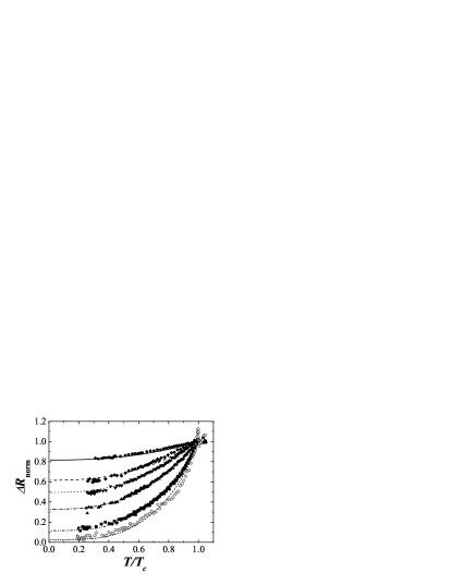
Figure 9: MR is plotted as a function of temperature $T/T_{c}$. The solid curves show theoretical results for the thickness of the SC, $L=$30, 40, 50, 60, 80, and 100 nm from top to bottom, where $k_{F}$ is taken to be $1\,{\rm\r{A}^{-1}}$ for Nb. The symbols show the experimental results by Gu et al.gu for the thickness of the Nb, $t_{Nb}$=30, 40, 50, 60, 80, and 100 nm from top to bottom.

Let us compare our theory with recent experimental results in Py/Nb/Py structures measured by Gu et al..gu The mean free path in the Nb film $l\sim 6$ nmgu is much smaller than the clean-limit coherence length $\xi_{0}\sim 40$ nmTinkham and therefore the Nb film is in the diffusive regime. In order to analyze the experimental results in the dirty Nb film, we need to extend the theory in the ballistic case to that in the diffusive case. The diffusive effect on the Andreev reflection is incorporated into our theory by replacing the penetration depth $\xi_{Q}$ in the ballistic theory with the penetration depth in the dirty-limit $\xi_{Q}^{D}$. Thus, the value of $\xi_{Q}(E=0)$ at $T=0$ obtained by fitting the experimental data is interpreted as the dirty-limit penetration depth $\xi_{Q}^{D}(E=0)\sim 1.2\sqrt{l/\xi_{0}}\,\xi_{Q}(E=0)$xiQD at $T=0$. Figure 9 shows the excess resistance $\Delta R=R_{\rm AP}-R_{\rm P}$ normalized by the value at (in the experiment, $T$ slightly above) $T_{c}$ ($\Delta R_{\rm norm}$) as a function of temperature. The solid curves indicate the calculated results and the symbols indicate the experimental ones.gu By fitting the calculated values to those of the experimental data, we obtain $\xi_{Q}^{D}(E=T=0)$ = 46, 36, 36, 33, 30, and 27 nm for the curves of $L$=30, 40, 50, 60, 80, and 100 nm, respectively, where $k_{F}$ is taken to be $1\,{\rm\r{A}^{-1}}$ for Nb.ashcroft The values of the penetration depth $\xi_{Q}^{D}(E=T=0)$ estimated by our theory become larger for the smaller thickness of the Nb film and are larger than the dirty-limit penetration depth in a bulk Nb $\sim\sqrt{\xi_{0}l}$ = 16.2 nm. This indicates that $\Delta$ in the Nb film is reduced compared to that in a bulk Nb. The suppression of $\Delta$ is due to the proximity effect. Actually, the height of the realistic superconducting gap depends on the position $z$ in the Nb film by the proximity effect. Here we interpret the value of $\Delta$ as the averaged value of the realistic superconducting gap with respect to $z$ in the Nb film. Gu et al. have obtained the dirty-limit penetration depth $\xi_{Q}^{D}(E=T=0)\sim 16.5$ nm by assuming that $\Delta R_{\rm norm}$ is proportional to $\exp(-t_{Nb}/\xi_{Q}^{D})$, where $t_{Nb}$ is the thickness of the Nb. This value of the penetration depth is comparable to those estimated by our theory.

Although we neglect the effect of spin relaxation on the MR in our theory, this assumption is justified as follows. In the Nb film in the Py/Nb/Py structure, the spin diffusion length $\lambda_{s}$ is about $50$ nm,gu while the penetration depth $\xi_{Q}(T=0)$ is about $27\sim 46$ nm at low energy. As seen in Fig. 5, $\xi_{Q}(T)$ is almost constant at low temperatures and shows the divergent behavior only near $T_{c}$, indicating that $\xi_{Q}$ is smaller than $\lambda_{s}$ in most of the temperature range below $T_{c}$. Therefore, the effect of the QP current penetration is dominated for the MR and the spin relaxation effect on the MR is neglected except in the close vicinity to $T=T_{c}$.

V Conclusion

The magnetoresistance in the ferromagnet/superconductor/ferromagnet double junction system is studied theoretically. The dependences of the magnetoresistance on the thickness of the superconductor, temperature, the exchange field of ferromagnets and the height of the interfacial barriers are understood by considering the Andreev reflection of spin-polarized current. Our theory shows good agreement with recent experimental results.

- (1) Spin Dependent Transport in Magnetic Nanostructures edited by S. Maekawa and T. Shinjo (Taylor and Francis, London and New York, 2002).
- (2) R. Meservey and P.M. Tedrow, Phys. Rep. 238, 173 (1994).
- (3) V.A. Vas’ko, V.A. Larkin, P.A. Kraus, K.R. Nikolaev, D.E. Grupp, C.A. Nordman, and A.M. Goldman, Phys. Rev. Lett. 78, 1134 (1997).
- (4) Z.W. Dong, R. Ramesh, T. Venkatesan, Mark Johnson, Z.Y. Chen, S.P. Pai, V. Talyansky, R.P. Sharma, R. Shreekala, C.J. Lobb, and R.L. Greene, Appl. Phys. Lett. 71, 1718 (1997).
- (5) N.-C. Yeh, R.P. Vasquez, C.C. Fu, A.V. Samoilov, Y. Li, and K. Vakili, Phys. Rev. B 60, 10522 (1999).
- (6) J.Z. Liu, T. Nojima, T. Nishizaki and N. Kobayashi, Physica C, 357-360, 1614 (2001).
- (7) C.D. Chen, W. Kuo, D.S. Chung, J.H. Shyu, and C.S. Wu, Phys. Rev. Lett. 88, 047004 (2002).
- (8) S. Takahashi, H. Imamura, and S. Maekawa, Phys. Rev. Lett. 82, 3911 (1999).
- (9) T. Yamashita, S. Takahashi, H. Imamura, S. Maekawa, Phys. Rev. B 65, 172509 (2002).
- (10) S. Takahashi, T. Yamashita, H. Imamura, S. Maekawa, J. Magn. Magn. Mater. 240, 100 (2002).
- (11) S. Takahashi and S. Maekawa, Phys. Rev. Lett. 88, 116601 (2002).
- (12) M.J.M. de Jong and C.W.J. Beenakker, Phys. Rev. Lett. 74, 1657 (1995).
- (13) K. Kikuchi, H. Imamura, S. Takahashi, and S. Maekawa, Phys. Rev. B 65, 020508(R) (2001).
- (14) H. Imamura, K. Kikuchi, S. Takahashi, and S. Maekawa, J. Appl. Phys. 91, 172509 (2002).
- (15) J.-X. Zhu, B. Friedman, and C.S. Ting, Phys. Rev. B 59, 9558 (1998).
- (16) I. Žutić and O.T. Valls, Phys. Rev. B 60, 6320 (1999).
- (17) S. Kashiwaya, Y. Tanaka, N. Yoshida, and M.R. Beasley, Phys. Rev. B 60, 3572 (1999).
- (18) R.J. Soulen Jr., J.M. Byers, M.S. Osofsky, B. Nadgorny, T. Ambrose, S.F. Cheng, P.R. Broussard, C.T. Tanaka, J. Nowak, J.S. Moodera, A. Barry, and J.M.D. Coey, Science 282, 85 (1998).
- (19) R.J. Soulen, Jr., M.S. Osofsky, B. Nadgorny, T. Ambrose, P. Broussard, S.F. Cheng, J. Byers, C.T. Tanaka, J. Nowack, J.S. Moodera, G. Laprade, A. Barry, and M.D. Coey, J. Appl. Phys. 85, 4589 (1999).
- (20) Y. Ji, G.J. Strijkers, F.Y. Yang, C.L. Chien, J.M. Byers, A. Anguelouch, Gang Xiao, and A. Gupta, Phys. Rev. Lett. 86, 5585 (2001).
- (21) G.J. Strijkers, Y. Ji, F.Y. Yang, C.L. Chien, and J.M. Byers, Phys. Rev. B 63, 104510 (2001).
- (22) S.K. Upadhyay, A. Palanisami, R.N. Louie, and R.A. Buhrman, Phys. Rev. Lett. 81, 3247 (1998).
- (23) A.F. Andreev, Sov. Phys. JETP 19, 1228 (1964).
- (24) V.L. Ginzburg and L.D. Landau, Zh. Eksperim. i Teor. Fiz. 20, 1064 (1950).
- (25) G.E. Blonder, M. Tinkham, and T.M. Klapwijk, Phys. Rev. B 25, 4515 (1982).
- (26) W.P. Pratt, Jr. ; private communication, J.Y. Gu, J.A. Caballero, R.D. Slater, R. Loloee, and W.P. Pratt, Jr., to be published in Phys. Rev. B.
- (27) P.G. de Gennes, Superconductivity of Metals and Alloys (W. A. Benjamin, New York, 1966), chap. 5.
- (28) W. Belzig, Arne Brataas, Yu.V. Nazarov and Gerrit E.W. Bauer, Phys. Rev. B 62, 9726 (2000).
- (29) C.J. Lambert, J. Phys.: Condens. Matter 3, 6579 (1991).
- (30) M. Tinkham, Introduction to Superconductivity (McGraw Hill, New York, 1996).
- (31) We assume that the dirty-limit penetration depth is expressed as by analogy with the clean-limit case, where is the dirty-limit GL coherence length. Using the relation ,Tinkham the dirty-limit penetration depth can be expressed as .
- (32) N. Ashcroft and N. Mermin, Solid State Physics (Saunders College Publishing, New York, 1976).