Transport properties of a modified Lorentz gas

Abstract

We present a detailed study of the first simple mechanical system that shows fully realistic transport behavior while still being exactly solvable at the level of equilibrium statistical mechanics. The system under consideration is a Lorentz gas with fixed freely-rotating circular scatterers interacting with point particles via perfectly rough collisions. Upon imposing a temperature and/or a chemical potential gradient, a stationary state is attained for which local thermal equilibrium holds for low values of the imposed gradients. Transport in this system is normal, in the sense that the transport coefficients which characterize the flow of heat and matter are finite in the thermodynamic limit. Moreover, the two flows are non-trivially coupled, satisfying Onsager’s reciprocity relations to within numerical accuracy as well as the Green-Kubo relations . We further show numerically that an applied electric field causes the same currents as the corresponding chemical potential gradient in first order of the applied field. Puzzling discrepancies in higher order effects (Joule heating) are also observed. Finally, the role of entropy production in this purely Hamiltonian system is shortly discussed.

I Introduction

One of the major motors of research in statistical physics has been the quest to understand the link between macroscopic phenomena and the underlying microscopic physics of a system. In particular, the origin of the macroscopic “laws” of thermodynamic transport is still one of the major challenges to theoretical physics. These phenomenological laws are known to describe accurately the processes of diffusion, heat conduction, viscosity among a host of other phenomena, and are fundamental to the quantitative description of macroscopic systems in general. However, the attempts to link these macroscopic laws to the underlying microscopic dynamics have not been conclusive thus far. From a mathematically rigorous point of view, very few results have been obtained bonetto01 . Indeed, to our knowledge, the validity of Fourier’s law has been proven analytically only for a very specific model in the limit of infinite dilution with finite mean free path lebowitz78 ; lebowitz82 . There have also been attempts to link transport phenomena to the chaotic properties of the underlying classical dynamics bunimovich80 ; and a connection between the rate of entropy production and the rate of contraction of phase space volume in thermostated (non Hamiltonian) systems has been pointed out chernov93 ; holian87 ; moran87 ; chernov93-2 .

Given this state of affairs, a common strategy is to propose and study systems which reproduce, in numerical simulations, the phenomena under consideration, and to attempt to determine how the physical ingredients of these models give rise to the macroscopic behaviour. However, the systems considered thus far have been either too complicated to shed much light upon the problem, or have actually failed to reproduce the macroscopic phenomenology. Attempts have been made, on one side, through the simulation of realistic many-body systems satisfying a thermostated dynamics (see for example evans86 ). These simulations have indeed been able to reproduce non-trivial transport phenomena. However, such studies do not provide a detailed understanding of the microscopic processes involved due to the excessive complexity of the system under study. The other numerical approach involves the study of transport in “simple systems”. Examples of these include: chains of anharmonic oscillators lepri97 and the so called ding-a-ling and ding-dong models casati84 ; prosen92 , among others. Of these, energy transport in the chains was shown to be “anomalous”. This is an euphemism indicating that energy transport cannot be described as a diffusive process and currents do not scale with the gradients in the expected way. In contrast, “normal” transport indicates that even in the thermodynamic limit, transport can accurately be described as a diffusive process and that the flux is proportional to the gradient as stated, say, in Fourier’s law. The ding-a-ling and ding-dong models, indeed do yield normal transport under certain conditions; however, they include geometric constraints that make even their equilibrium properties an extremely complicated affair. As we shall see, the knowledge of such equilibrium properties is often useful, which is why we consider it important to have a model where these are explicitly known.

One particularly thorny problem in attempting to reproduce the phenomenological laws of thermodynamic transport, is that these apply to systems which are characterized by local thermodynamic equilibrium (LTE) rondoni02 ; cohen02 . That is, systems that are not in equilibrium, but for which the intensive thermodynamic variables are well defined at each point of the system, and the relations amongst these variables are the same as in equilibrium thermodynamics. Thus, results have been obtained concerning “diffusive” (normal) energy transport in the Lorentz gas alonso99 . Yet this system is not described by LTE dhar99 . It is therefore not clear what precise meaning can be attached to the local temperature appearing in Fourier’s law in this situation.

Under these circumstances, the minimal ingredients required in the microscopic physics of a simple system to attain normal thermodynamic transport in low dimensions are presently still under discussion bonetto01 ; hu98 ; prosen00 . However, we believe that ideal candidate models should possess the following features:

1. The microscopic physics should be defined in terms of reversible Hamiltonian dynamics, since this is the nature of known fundamental processes. In particular, reversible systems showing an average rate of phase space contraction, while of considerable interest for simulating transport, do not provide a fundamental microscopic model.

2. The equilibrium properties of the model should be well understood.

3. When driven weakly out of equilibrium, they must be consistent with the hypotheses of LTE and, of course, they must give rise to realistic macroscopic transport.

In this work we present a detailed description and extensive simulations of the equilibrium and transport properties of a simple reversible Hamiltonian model system which we believe is an ideal candidate to begin to unravel the puzzle of thermodynamic transport. The first results concerning some of the transport features of this model were presented in mejia01 . In Section II, we present a detailed description and discussion of the model. We show that its equilibrium statistical mechanics is simply that of an ideal gas.

In order to carry out the equilibrium simulations, as well as to study the transport properties of the model when the system is driven out of equilibrium, it is necessary to couple the system to thermo-chemical baths. We describe the model baths we have implemented to do this in Section III.

In Section IV we corroborate through simulations that the equilibrium state of the system in the three canonical ensembles is indeed an ideal gas. We also present numerical evidence to show that, when subjected to a weak temperature and/or chemical potential gradient, our systems reaches a non-equilibrium steady state (NSS) which is characterized by LTE. In this situation, our model supports both heat and matter flows. We show in Section V that these flows are characterized by transport coefficients which are independent of system size (that is, transport is normal), and that the corresponding transport coefficients satisfy Onsager’s reciprocity relations. The fact that the system is homogeneous in energy allows the prediction of the dependence of the transport coefficients on the temperature. We also establish numerically their dependence on the particle density and discuss briefly the effects of subjecting the system to a magnetic field. In Section VI we verify that the Green-Kubo formulas connecting transport coefficients with time correlation functions apply for this system to within numerical precision, and we compare the effect of an applied electric field with that of an applied chemical potential gradient, which, to linear order, should induce the same flows in the system. In Section VII a brief discussion of the applicability of microscopic interpretations of entropy production as motor of transport in this system. Finally we present a brief summary and mention how this model can be modified to study other physical transport problems from a microscopic approach.

II Definition of the model

In alonso99 , a Lorentz gas model with elastic collisions was used to study heat transport in a quasi-one dimensional channel placed between two thermal reservoirs at different nominal temperatures. While the results were consistent with some sort of “diffusive” energy transport, identification with Fourier’s law was unfounded: the system does not satisfy the hypothesis of LTE and, therefore, one cannot define a local temperature, as was shown in dhar99 . There, the authors argue that the system does not attain LTE due to the existence of an infinite number (in the thermodynamic limit) of conserved quantities in the dynamics. Indeed, the energy of each particle is conserved throughout the evolution of the system. This, in turn, implies a breakdown of ergodicity and the resulting process is closer to “colour” diffusion than to heat transport.

The model we study in this work, introduced in mejia01 , is a modification to the usual Lorentz gas model in which the scatterers are allowed to exchange energy with a set of (non-interacting) point particles of mass $m$ through the scattering events. The geometry we consider is that of a periodic Lorentz gas in which the hard disc scatterers of radius $R$ are fixed on a triangular lattice, the details of which are discussed below. The possibility of energy exchange is achieved as follows: each disc is a free rotator with a moment of inertia $\Theta$, and scattering proceeds according to rules characterizing “perfectly rough” collisions, that are reversible, conserve total energy and angular momentum. These collision rules are given by the following formulas, which relate the normal and tangential components of the particle’s velocity ${\bf v}$ with respect to the disc’s surface, and the disc’s angular velocity $\omega$ before (unprimed quantities) and after (primed quantities) the collision

$$v_{n}^{\prime} = -v_{n}\,$$

$$v_{t}^{\prime} = v_{t}-\frac{2\eta}{1+\eta}(v_{t}-R\omega)\,$$ (1)

$$R\omega^{\prime} = R\omega+\frac{2}{1+\eta}(v_{t}-R\omega)\ .$$

These rules define a deterministic, time-reversible, canonical transformation at each collision. The parameter $\eta$, defined as the ratio between the moment of inertia of the disc and the mass of the particle times the square radius of the disc:

$$\eta=\frac{\Theta}{mR^{2}}\ ,$$ (2)

is the only relevant adimensional parameter characterizing the collision. It determines the energy transfer between discs and particles in a collision. For finite values of $\eta$, particles in the system may exchange energy among each other through the discs, even though they do not interact directly. This simple energy exchange mechanism overcomes the objections raised in dhar99 and permits the system to reach thermodynamical equilibrium, as we will see in Section IV. As $\eta\to 0$, the rotational energy of the scatterers becomes negligible and the collision becomes perfectly elastic, recovering the dynamics of the usual Lorentz gas model. For $\eta\to\infty$, the energy of the scatterers is unaffected by the collisions with the particles, and the angular velocity of the scatterers remains constant. In this limit, once again, the system does not equilibrate. Thus, in either limit, the energy-mediating effect is suppressed and thermodynamical equilibrium is not reached. In the following, unless the contrary is explicitly stated, we shall always be dealing with the case $\eta=1$, since that is a value of $\eta$ for which energy exchange, and therefore equilibration, is quite efficient.

The geometric disposition of the scatterers in the systems we study in this work is indicated in Fig. 1. The centers of the scatterers are fixed on a triangular lattice, along a narrow channel of height $2W$, where $W$ is the distance between the centers of the scatterers. For convenience, this distance was chosen as $W=4R/\sqrt{3}$ (known in the literature as the critical horizon), which is the largest separation for which a particle cannot travel arbitrarily large distances without undergoing a collision. In this geometry, a set of non-interacting point particles of mass $m$ moves freely between collisions with the hard discs. In the vertical direction the channel contains two discs and periodic boundary conditions are imposed.

The fact that we put two discs in the vertical direction merits comment as, in the simpler “single cell” geometry with periodic boundary conditions, spurious effects may arise from multiple successive scatterings of one particle with the same disc. Some of these effects have been observed in klages00 , where the same set of collision equations has been used to model a deterministic thermostat. We have verified that if one considers a system consisting of one cell with periodic boundary conditions, containing a single scatterer and a single particle, the resulting dynamics gives rise to regular structures in the phase space of the particle. In this situation, the system does not appear to be ergodic for arbitrary values of $\eta$. We also noted that, if instead of periodic boundary conditions one considers specular reflections at the boundaries, the effect in the particle’s trajectory is a “randomization” of the tangential component of the particle’s velocity in the next collision with the disc, recovering a seemingly ergodic phase space. Though we believe that the presence of other particles will destroy the regular structures that appear in the single particle case, we decided to avoid the possibility of multiple consecutive collisions of a particle with the same disc by placing two discs in the vertical direction.

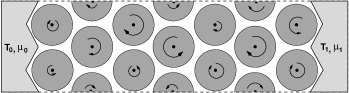
Figure 1: Schematic illustration of the scatterer geometry: the scatterers are disposed on a triangular array with finite horizon to avoid infinitely long trajectories. For matters of convenience, in this work the separation between scatterers has been set to have the critical horizon. Periodic boundary conditions are used in the vertical direction. To avoid spurious effects arising from multiple consecutive scatterings of a particle off the same disc, we have put two discs on each vertical. To study the dependence with system size, the length L of the sample is varied. The quoted length is the number of discs.

A central aspect of this model is that its equilibrium properties are still trivial, even though, strictly speaking, it is an interacting many particle system. Indeed, in spite of the modified collision rules, the energy of the system is given by

$$E=m\sum\limits_{particles}\frac{{\bf v_{i}}^{2}}{2}+\Theta\sum\limits_{rotors}\frac{\omega_{\alpha}^{2}}{2}\ .$$ (3)

Thus, all statistical mechanics calculations for this system coincide with those of a system consisting of a two dimensional ideal gas plus a collection of non-interacting free rotors. Hence, a first test for the system is to verify that it equilibrates to a state in which its statistical properties are indeed those predicted by equilibrium statistical mechanics. In particular, in microcanonical simulations, the particle velocities should reach Maxwellian distributions at a uniform “temperature” consistent with the equipartition theorem homogeneity . These temperatures should also characterize the distribution of angular velocities of the rotating scatterers. The same should be true in canonical and grand canonical simulations, where the temperature and particle density (or, more formally, the chemical potential divided by the temperature) are now those established by the values of the baths. Furthermore, the equations of state characterizing ideal gases should describe the thermodynamics of our system. If any of these tests fails, it could be argued that the system fails to equilibrate probably due to a lack of ergodicity. Unfortunately, passing all the tests does not prove that the system is ergodic. We have not succeeded in showing rigorously that this system is ergodic. However, these numerical tests are fairly stringent: we shall see that for the case of an imposed external magnetic field, where ergodicity is known to be violated, an effect indeed appears in the energy distribution function of the particles.

III Thermo-chemical Baths

In numerical studies of statistical mechanics systems in general, and in those on the microscopic origin of macroscopic transport in particular, it is necessary to define models for the thermodynamical reservoirs in addition to the dynamics of the system. The design of these reservoirs and the way these interact with the system, has several subtleties that can produce confusing and, very often, wrong results, as has been pointed out in koplik98 ; hatano99 . In this Section, we explain the design of a stochastic model that simulates a thermo-chemical bath, which is able to exchange energy and particles with the system at fixed nominal values for the temperature $T$ and chemical potential $\mu$.

The heat and matter reservoir is taken to be an infinite ideal gas at temperature $T$ and density $\rho$ which is placed in direct contact with the system being studied. This is achieved by assuming that the wall separating the system from the reservoir is perfectly transparent to particles impinging on it from either side. Of course, it is not necessary to simulate explicitly the infinite ideal gas which acts as the thermodynamical reservoir, instead, we can implement this set up using the following rules: whenever a particle of the system impinges on the boundary which separates it from the bath, it is removed. On the other hand, with a frequency $\gamma$, particles are generated at the boundary, with a velocity distribution

$$P_{n}(v_{n}) = \ \frac{m}{T}|v_{n}|\exp\left(-\frac{mv_{n}^{2}}{2T}\right)\ ,$$

$$P_{t}(v_{t}) = \sqrt{\frac{m}{2\pi T}}\exp\left(-\frac{mv_{t}^{2}}{2T}\right)\ ,$$ (4)

reflecting the assumption that the bath is an ideal gas (here and in the following, we take the particle mass and Boltzmann’s constant equal to one). The choice of $T$ in these equations defines the nominal temperature of the bath. Moreover, this way of implementing the thermo-chemical baths also fixes a nominal value for their chemical potential. Again, as the bath is an ideal gas, the rate $\gamma$ is given by:

$$\gamma=\frac{1}{\sqrt{2\pi}}\rho~{}T^{1/2}\ .$$ (5)

Thus, we can express the chemical potential of the bath in terms of the parameter $\gamma$ as:

$$\mu=T\ln\left(\frac{\lambda_{0}\gamma}{T^{3/2}}\right)\ ,$$ (6)

where $\lambda_{0}$ is an irrelevant constant.

Equations (4), (5) and (6) completely define the algorithm for the stochastic emission process of the thermo-chemical baths used in the simulations, and allow us to control the chemical potential and temperature of the walls by varying the rate $\gamma$ and the temperature. These walls were used for grand canonical simulations in equilibrium and coupled heat and matter transport simulations in the NSS.

To simulate the canonical ensemble in equilibrium and pure heat flow in the NSS, diathermal impermeable walls are required. These were achieved by reflecting each particle that impinged on the wall back into the system, with its velocity updated according to the distribution function (4), which again defines the nominal temperature of the thermal bath.

Finally, in order to perform simulations in the microcanonical ensemble, insulating walls are required. We have simulated these either by simply considering that the particles always perform elastic specular reflection at the boundary, or by having no walls at all and considering periodic boundary conditions.

A generalized model for thermo-chemical bath, as well as a general approach allowing to verify the validity of a given procedure for generating such baths is given in Appendix A.

IV Equilibrium and Local thermal equilibrium

In this section we show that the system described in Section II reaches a well defined equilibrium state for the different equilibrium ensembles. For each ensemble we place the system in contact with the appropriate wall, as described in the previous Section. However, as expected, the equilibrium state that the system reaches does not depend on the particular choice of the ensemble. Furthermore, when the nominal values for the thermodynamical quantities fixed by the baths impose a gradient in temperature and/or in the chemical potential, our model reaches a well defined steady state.

In order to show that our model reaches a satisfactory equilibrium state we have measured the velocity distribution of the particles $P(v)$ and the angular velocity distribution of the discs $P(\omega)$ in a microcanonical simulation in which the particles undergo specular reflections with the walls at the left and right extremes of the channel. We have fixed the energy of the system and distributed it randomly among discs and particles. After some relaxation time the mean energy per particle is twice the mean energy per disc, thus satisfying the equipartition theorem. In Fig. 2, the measured distributions $P(v)$ and $P(\omega)$ are shown. The solid line is the corresponding Boltzmann distributions at the expected temperature ($T=150$ in arbitrary units). The agreement indicates that both discs and particles have reached a state consistent with the predictions of equilibrium statistical mechanics. This agreement also allows us to relate the average energy per particle with the temperature, which would have been unfounded otherwise.

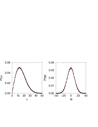
Figure 2: Discs angular velocity distribution $P(\omega)$ and particles velocity distribution $P(v)$ obtained in a microcanonical simulation with $30$ particles in a channel of length $L=30$. The solid lines correspond to the Boltzmann distribution at the expected temperature $T=150$.

We have computed the particle density and temperature profiles in the following way: We divide the channel in ${\mathcal{R}}$ disjoint slabs of width $\Delta x=L/{\mathcal{R}}$. As before, $L$ is the length of the channel in the $x$-direction. The particle density, $n(x)$, in each slab is computed as the time average

$$n(x)dx=\frac{1}{{\mathcal{T}}}\int_{0}^{\mathcal{T}}\sum_{i=1}^{N}\delta(x-x_{i}(t))\,dt\,dx\ ,$$ (7)

where $x_{i}(t)$ is the position of the $i$-th particle at time $t$ and $N$ is the total number of particles in the channel that, in the case of a grand canonical situation, depends on time. The time average is performed after the steady state has been reached.

Similarly, the time averaged energy density $\varepsilon(x)$ is computed as

$$\varepsilon(x)dx=\frac{1}{{\mathcal{T}}}\int_{0}^{\mathcal{T}}\sum_{i=1}^{N}E_{i}(t)\delta(x-x_{i}(t))\,dt\,dx\ .$$ (8)

Here $E_{i}(t)$ is the energy of the $i$-th particle at time $t$. From (7) we obtain the particle’s density profile $\rho(x)$ as the mean number of particles found in the slab which contains the position $x$

$$\rho(x)=\int_{\Delta x}n(x)\,dx\ .$$ (9)

The integral in (9) is taken over the domain of the slab that contains position $x$. Analogously, the average particle energy $E(x)$ at the slab containing position $x$ is given by

$$E(x)=\int_{\Delta x}\varepsilon(x){\mathrm{d}}x\ .$$ (10)

With (9) and (10), we calculate the particle temperature profile $T(x)$ as

$$T(x)=\frac{E(x)}{\rho(x)}\ .$$ (11)

In Fig. 3, we show the temperature profile obtained in a canonical simulation where both baths were set to the same nominal temperature. The temperature obtained according to (11) has additionally been averaged over an ensemble of $500$ different realizations. The number of particles was set to $N=30$ in a channel of length $L=30$. We observe that the particles reach an equilibrium state characterized by a constant temperature along the channel which coincides with the nominal values of the baths’ temperature. Moreover, the open circles in Fig. 3 correspond to the time averaged energy of the discs. The agreement of both profiles indicates equilibration between particles and discs.

In this equilibrium state, the particle’s density profile (not shown), is also flat. The same behaviour was also obtained in grand canonical simulations, as was to be expected from the equivalence of the different statistical ensembles.

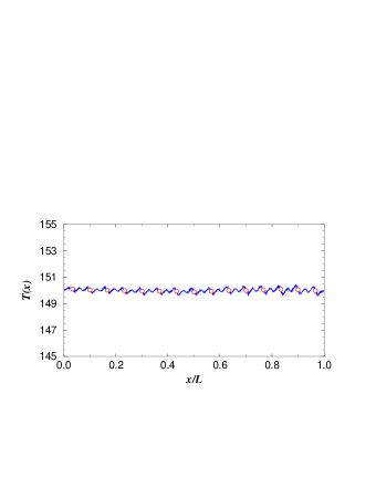
Figure 3: Particle’s temperature profile $T(x)$ for a canonical simulation. The number of particles was $N=30$ and $L=30$. The nominal temperature in both baths was set to same value $T=150$. The open circles correspond to the time averaged temperature of the discs.

Let us finally note the following: we have also performed simulations involving an external magnetic field. In this case, it is immediately clear that the system is not ergodic. Indeed, there exist isolated circular orbits which do not touch any disc. Since particles do not interact directly, any particle originally on one of these orbits will remain for ever. Similarly, this set of orbits cannot be reached from initial conditions for which each particle touches one disc at least once. Of course, for small fields, the orbits that do not touch any scatterer only occur when the particle’s kinetic energy is low, but since the particles can exchange energy with the discs, the kinetic energy of a particle can come arbitrarily close to zero, and there will be regions that become unreachable for this particle. There is thus a true lack of ergodicity for this system for arbitrary (non zero) magnetic fields and at all temperatures, although the effect becomes weaker as the field decreases. We have plotted in Fig. 4 the distribution of particle energies in the microcanonical ensemble and clear deviations from the Boltzmann distribution are observed. This comes as an indication that the tests we have applied should disclose a lack of ergodicity in the system without magnetic field if such were present.

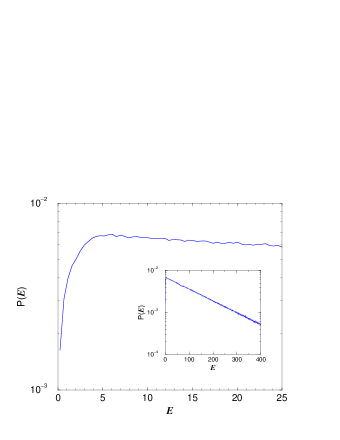
Figure 4: Particle’s energy distribution obtained from a microcanonical simulation with an applied external magnetic field. The magnitude of the field $B$ is such that $qB/mc=10$, where $q$ and $m$ are the electric charge and mass of the particles respectively and $c$ is the speed of light. The lack of low energy particles is evident. In the inset, ${\mathrm{P}}(E)$ is shown on a larger energy domain.

We now turn to the more interesting out of equilibrium situation. In these simulations we connect the two ends of the system with two different baths, each of which has given values of the chemical potential and the temperature. To drive the system out of equilibrium, the nominal values of the temperatures and chemical potentials of these baths are set to differ by fixed amounts. Under these conditions, the system is allowed to evolve until a non-equilibrium steady state (NSS) develops. In Fig. 5, we show results for a typical simulation; the profile corresponds to the average energy per particle for discs and particles obtained in a channel of length $L=30$. The temperature difference of the baths was set to $\Delta T=20$ around a central value $T=150$, with a chemical potential difference of $\Delta(\mu/T)=-0.2$. The profile of the average energy per particle is linear and coincides at the boundaries with the nominal baths’ temperature. As in equilibrium, in the steady state discs and particles locally equilibrate to the same value of the local mean energy per particle, giving a first indication of the establishment of LTE. As we will show further on, we will be justified in identifying the mean kinetic energy per particle with the local temperature.

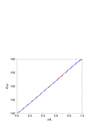
Figure 5: Temperature profile $T(x)$ with temperature and chemical potential gradients. The nominal values for the baths’ temperature are $T_{0}=140$ and $T_{1}=160$ with an end-to-end chemical potential difference of $\Delta(\mu/T)=-0.2$. The mean number of particles was $\approx 25.2$ in a channel of length $L=30$. The open circles correspond to the mean kinetic energy of the scatterers.

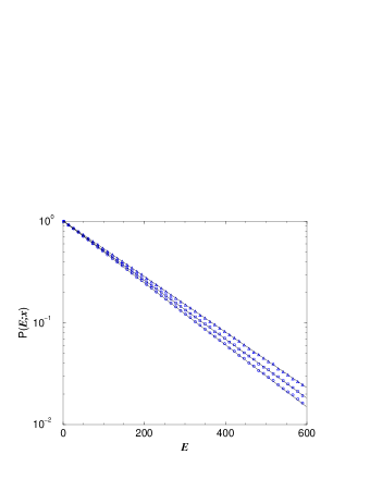
Figure 6: Semi-logarithmic plot of the particle’s energy distribution $P_{x}(E)$ at different positions along a channel obtained from the simulation described in Fig. 5. The different curves correspond to a fit to a Boltzmann distribution for each position. From these fits, we obtain the temperatures: $T=142.69$ at $x/L=0.1333$ (circles), $T=149.70$ at $x/L=0.4666$ (squares) and $T=158.69$ at $x/L=0.9333$ (triangles). The curves have been re-scaled for clarity.

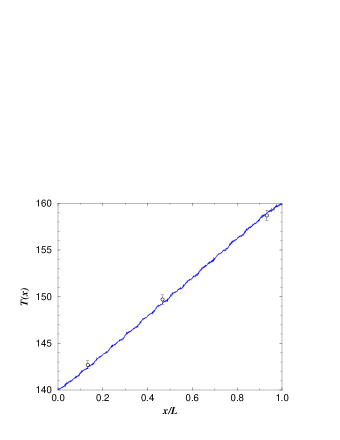
Figure 7: Temperature profile of Fig. 5 compared with the temperatures (open circles) obtained from the fit to the Boltzmann distribution of $P(E;x)$ shown in Fig. 6.

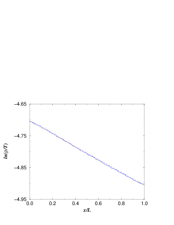
Figure 8: The quantity $\ln(\rho/T)$ (solid line) as a function of the position $x$ computed from the density and temperature profiles obtained in the simulation described in Fig. 5. The dashed line corresponds to a linear profile of the chemical potential $\mu/T$ joining its nominal values in the baths as obtained from (6). The solid line has been shifted from its obtained numerical value for a better comparison.

We now turn to the verification that LTE holds for our system. The assumption of LTE consists in the following: in every “infinitesimal” volume element one can define thermodynamic variables in the usual way and these are related to each other through the relations which hold for the system at equilibrium. It should be emphasized from the outset that this assumption is never exact: there always exist corrections of the order of the gradients imposed on the system. However, by choosing sufficiently small gradients it is always possible to reach a situation in which a definition of the temperature and density variables as if the volume element was in equilibrium, leads to reasonable values for the local chemical potential. Let us first discuss the issue of defining the temperature: in thermal equilibrium it is well known that the particle energies have a Boltzmann distribution. We may therefore define temperature as the parameter characterizing this distribution, arguing that temperature is ill-defined if the distribution is not Boltzmann. To this end we have computed the energy distribution of the gas of particles $P(E;x)$ as they cross a narrow slab centered at some position $x$. In Fig. 6, we show (in symbols), the results for $P(E;x)$ measured at three different positions for the same simulation described in Fig. 5. At each position the distribution $P(E;x)$ is consistent with the Boltzmann distribution, thus indicating that the gas of particles behaves locally as if it was in equilibrium at some temperature $T(x)$. If we determine the temperature $T(x)$ by a fit of $P(E;x)$ to the Boltzmann distribution and compare these values with the mean energy per particle profile of the system shown in Fig. 5, we see in Fig. 7 that $T(x)$ coincides with the mean energy of the particles measured locally at the position $x$. Thus, in the steady state, a local Boltzmann distribution is established. Therefore, the identification of the mean energy per particle with the local temperature in this model is justified.

In Fig. 8, we now compare the dependence on $x$ of the quantity $\ln(\rho/T)$ with a linear profile between the nominal values of $\mu/T$ in the thermo-chemical baths for the same simulation. The agreement between both curves (the profile of $\ln(\rho/T)$ has been shifted for comparison), indicates that $\Delta\mu/T=\Delta\ln(\rho/T)$, supporting the fact that the gas of particles inside the channel behaves locally as an ideal gas. By this we mean that the relation between the chemical potential, the density and the temperature for an ideal gas in equilibrium holds good locally to an excellent approximation in the NSS under study.

There is, however, an obvious discrepancy: since the NSS generally carries a non-zero particle current, it is clear that the average velocity is non-vanishing, thereby contradicting the Maxwellian distribution for the velocities. This is shown in detail in Fig. 9 where the deviation from the Maxwell distribution given in terms of ratio $\Gamma(v_{x})=\{P(v_{x})-P(-v_{x})\}/P(v_{x})$ is plotted. The systematic positive value of $\Gamma(v_{x})$ is an indication that the average velocity is greater than zero lamberto . This velocity, however, is proportional to the particle current, and hence to the gradients. Since these must be assumed small for LTE to hold, it is a small effect, which vanishes in the relevant limit. At this point, it is worthwhile to make the following point, when one states that a model such as that defined in casati84 does not satisfy LTE, it means that the deviations from LTE do not decrease as the gradients. In that case, for example, they only decay as the imposed temperature difference goes to zero, which in the thermodynamic limit is a much more stringent condition.

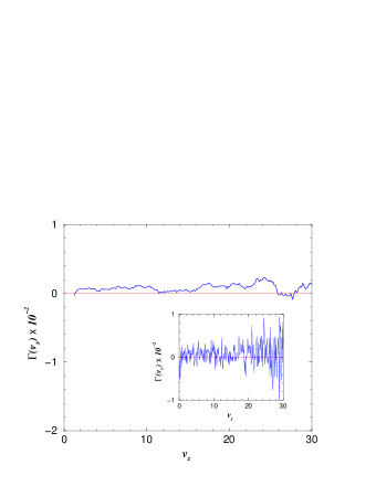
Figure 9: Window average of the deviation from the Maxwell distribution given in terms of the ratio $\Gamma(v_{x})=\{P(v_{x})-P(-v_{x})\}/P(v_{x})$ for a simulation with $\Delta(\mu/T)=-0.06$ and $T$ constant in a channel of length $L=30$. In the Inset, the original result for $\Gamma(v_{x})$ is shown.

V Normal transport and Onsager reciprocity relations

Having shown that we can assign an unambiguous meaning to local thermodynamical quantities in the non equilibrium steady states reached by the system, we can now study the transport properties of our systems, and whether these comply with the predictions of irreversible thermodynamics.

From the general theory of irreversible processes, to linear order, the heat and particle currents ${\mathrm{J}}_{u}$ and ${\mathrm{J}}_{\rho}$ can be written as follows (see e.g. mazur84 ):

$${\mathrm{J}}_{u} = L_{uu}\nabla\frac{1}{T}-L_{u\rho}\nabla\frac{\mu}{T}\ ,$$

$${\mathrm{J}}_{\rho} = L_{\rho u}\nabla\frac{1}{T}-L_{\rho\rho}\nabla\frac{\mu}{T}$$ (12)

and the Onsager reciprocity relations read in this case

$$L_{u\rho}=L_{\rho u}\ .$$ (13)

We now wish to show a central feature of our model: namely that its transport properties are normal, meaning that the various transport coefficients appearing in (12) do not depend on the length of system, and are thus well defined in the thermodynamical limit. In Fig. 10 we show the dependence of the currents on the length $L$ of the system, for a typical realization, in which we keep the differences $L\nabla T$ and $L\nabla\mu/T$ fixed as we vary the system size. The $1/L$ dependence observed confirms that transport is normal.

In order to obtain the value of the coefficients in (12), it is enough to perform two simulations: Fixing the value of $\nabla T$ and setting $\nabla(\mu/T)=0$ yields $L_{uu}$ and $L_{\rho u}$ from the direct measurement of the energy and particle flows, while setting $\nabla T=0$ and fixing $\nabla(\mu/T)$ gives $L_{u\rho}$ and $L_{\rho\rho}$. We have performed simulations with temperature and chemical potential differences up to 20% of the minimal nominal values at the walls, and in all cases we have found normal transport consistent with (13).

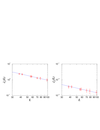
Figure 10: Size dependence of the heat and matter currents for simulations with a fixed temperature difference, $\Delta T=20$, and $\mu/T$ constant. The dotted lines corresponds to $1/L$ scaling.

In Fig. 11, we show the particle’s temperature and chemical potential profiles obtained from a simulation with constant $\mu/T$ and a temperature difference of $\Delta T=10$ around $T=150$ in a channel of length $L=30$ averaged over 470 realizations. After the steady state has been reached, we found that both a heat current and a particle current were driven by the temperature gradient. From (12) we obtained the following values for the Onsager coefficients:

$$L_{uu} = (0.7920\pm 0.0050)\rho T^{5/2}$$

$$L_{\rho u} = (0.1271\pm 0.0017)\rho T^{3/2}\ .$$ (14)

From the complementary simulation (see Fig. 12), where temperature is kept constant at $T=150$ and a chemical potential gradient is imposed with $\Delta(\mu/T)=-0.06$ we obtained

$$L_{u\rho} = (0.1272\pm 0.0048)\rho T^{3/2}$$

$$L_{\rho\rho} = (0.1050\pm 0.0030)\rho T^{1/2}\ .$$ (15)

In (V) and (V) we have written the explicit dependence of the Onsager coefficients on the particle’s density $\rho$ and temperature $T$. The temperature dependences arise from simple dimensional analysis given the fact that the system is homogeneous in energy, or equivalently, that it has no proper time scale. The same cannot be said of the density, but the obtained linear dependence shown in Fig. 13, at least in this range of density values, is not too surprising.

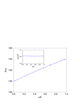
Figure 11: Particle’s temperature profile for a simulation where the quantity $\mu/T$ is kept constant. The nominal values for the baths’ temperature are $T_{0}=145$ and $T_{1}=155$ in a channel of length $L=30$. In the inset, the profile of $\mu/T$ as calculated from (6) with $\mu_{0}=1$ is shown to corroborate its constant value along the channel.

The obtained values for the symmetric coefficients $L_{\rho u}$ and $L_{u\rho}$ confirm (13) to within our numerical accuracy.

As a consistency check, we have also studied a “canonical” situation, in which we suppressed absorption and emission of particles at the walls while still allowing heat exchange. In this situation there is no flow of matter in the steady state. The relationship between heat flow and temperature gradient becomes ${\mathrm{J}}_{u}=\kappa\nabla T$, with $\kappa$ given by the following expression:

$$\kappa=\frac{L_{uu}L_{\rho\rho}-L_{u\rho}L_{\rho u}}{T^{2}L_{\rho\rho}}\ .$$ (16)

This relationship was found to hold to good accuracy, thus confirming the validity of our “grand canonical” simulations by which the $L$’s were evaluated. We remark that the coupling between the two currents in the NSS is non-trivial in the following sense: in a “canonical” simulation, the simplest assumption for the dependence of the density on the position is that the trajectory of each particle covers the sample uniformly. Then the local temperature merely determines the speed at which the orbit is being traversed. This would imply that in such a situation, the particle density should scale inversely with the average velocity, that is

$$\rho(x)T(x)^{1/2}=const\ .$$ (17)

In terms of the transport coefficients defined in (12), (17) is equivalent to $L_{\rho u}=(d+1)TL_{\rho\rho}/2$, where $d$ is the dimension of the system. This relation corresponds to a system for which all transport arises from uncorrelated Markovian motion of the particles, as in the Knudsen gas reichl88 . However, (17) does not hold in our system as we always find a small but systematic spatial variation in this quantity, the size and sign of which depend on the value of $\eta$. Thus, our system cannot be accurately described in such a simple manner.

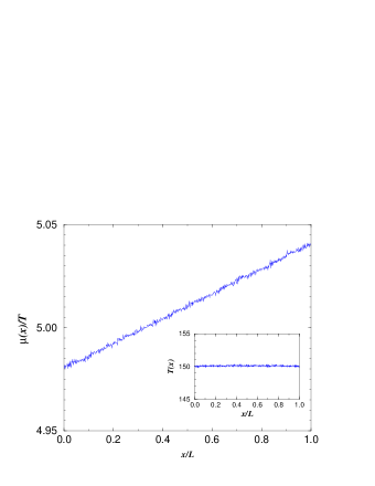
Figure 12: Profile of the quantity $\mu/T$ as calculated from (6) with $\mu_{0}=1$ for a simulation where the nominal values of the baths’ temperature are set to the same value $T=150$. with an end-to-end chemical potential difference of $\Delta(\mu/T)=-0.06$ in a channel of length $L=30$. In the inset, the particle’s temperature profile is shown.

Despite the fact that the dynamics of the system is not ergodic when an external magnetic field is applied, we have performed systematic simulations for several values of the magnetic field. In particular, we have measured both the matter and the energy currents appearing in the direction perpendicular to the applied thermodynamical gradients (the so-called Righi-Leduc effect, which is the thermal analog of the Hall effect mazur84 ). Even when a magnetic field is applied, the existence of the up-down symmetry in the system makes the dynamics equivalent to a situation where time-reversal symmetry holds. Due to this situation we are not able to verify the validity of the Onsager–Casimir relations which are the generalization of the Onsager relations when time-reversal symmetry is broken. Nevertheless, we have verified that all cross $L$-coefficients satisfy the Onsager relations to within numerical accuracy. The validity of the Onsager–Casimir relations deserves further investigation.

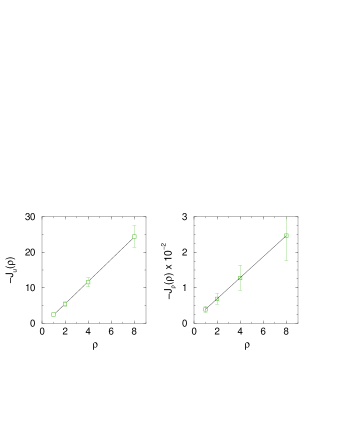
Figure 13: Density dependence of the particle ${\mathrm{J}}_{\rho}$ and heat ${\mathrm{J}}_{u}$ currents. Each symbol in these plots correspond to the averaged fluxes obtained from a simulation with constant $\mu/T$ and a temperature gradient for which $T_{0}=145$ and $T_{1}=155$ in a channel of length $L=30$. The lines correspond to linear fits.

VI Green-Kubo formalism

Another interesting question we are able to address with our system is whether the Green-Kubo relations hold. These relate the phenomenological collective transport coefficients with the equilibrium time correlation functions of microscopic dynamical variables.

As finite size effects limit the range of validity of the Green-Kubo relations, we begin by presenting a derivation of these relations which is appropriate to our finite length system self-diffusion . Starting from the phenomenological transport equations (12), and using the fact that the gas of particles is an ideal gas, we express (12) in terms of the gradients of the energy density $u$ and particle density $\rho$:

$${\mathrm{J}}_{u} = \frac{1}{\rho T}\left(L_{u\rho}-\frac{L_{uu}}{T}\right)\nabla{u}+\frac{1}{\rho}\left(\frac{L_{uu}}{T}-2L_{u\rho}\right)\nabla{\rho}\ ,$$

$${\mathrm{J}}_{\rho} = \frac{1}{\rho T}\left(L_{\rho\rho}-\frac{L_{\rho u}}{T}\right)\nabla{u}+\frac{1}{\rho}\left(\frac{L_{\rho u}}{T}-2L_{\rho\rho}\right)\nabla{\rho}\ .$$

As the analysis is restricted to the linear regime, the factors of $\rho$ and $T$ appearing in the coefficients of the gradients are taken as constants. Using energy and mass conservation, we obtain from (VI)

$$\frac{\partial}{\partial t}\left(\begin{matrix}u\\ \rho\\ \end{matrix}\right)=\mathbb{A}\nabla^{2}\left(\begin{matrix}u\\ \rho\\ \end{matrix}\right)\ ,$$ (19)

where the matrix $\mathbb{A}$ is the matrix of coefficients whose elements can be readily identified from (VI).

Applying a Fourier transform in space to (19) we obtain

$$\left(\begin{matrix}\hat{u}_{k}(t)\\ \hat{\rho}_{k}(t)\\ \end{matrix}\right)=e^{-tk^{2}\mathbb{A}}\left(\begin{matrix}\hat{u}_{k}(0)\\ \hat{\rho}_{k}(0)\\ \end{matrix}\right)\ ,$$ (20)

where $\hat{u}_{k}(t)$ and $\hat{\rho}_{k}(t)$ are the $k$ Fourier components of $u(x,t)$ and $\rho(x,t)$ evaluated at time $t$. Now we take the exterior product of (20) with the vector $(\hat{u}_{k}^{*}(0)\ \hat{\rho}_{k}^{*}(0)$ and average over the ensemble of equilibrium realizations to obtain

$${\mathbb{C}}_{k}(t)=e^{-tk^{2}{\mathbb{A}}}{\mathbb{U}}_{k0}\ .$$ (21)

The matrices ${\mathbb{C}}_{k}(t)$ and ${\mathbb{U}}_{k0}$ consist of correlation functions of the densities given by

$${\mathbb{C}}_{k}(t)=\left(\begin{matrix}\left<\hat{u}_{k}(t)\hat{u}_{k}^{*}(0)\right>&\left<\hat{u}_{k}(t)\hat{\rho}_{k}^{*}(0)\right>\\ \left<\hat{\rho}_{k}(t)\hat{u}_{k}^{*}(0)\right>&\left<\hat{\rho}_{k}(t)\hat{\rho}_{k}^{*}(0)\right>\\ \end{matrix}\right)$$ (22)

and

$${\mathbb{U}}_{k0}=\left(\begin{matrix}\left<|\hat{u}_{k}(0)|^{2}\right>&\left<\hat{u}_{k}(0)\hat{\rho}_{k}^{*}(0)\right>\\ \left<\hat{\rho}_{k}(0)\hat{u}_{k}^{*}(0)\right>&\left<|\hat{\rho}_{k}(0)|^{2}\right>\\ \end{matrix}\right)\ .$$ (23)

The above correlation functions were derived explicitly as forward time correlation functions; however, as they pertain to the stationary state of the system, we can extend them backwards in time as even functions. Having done this, the Fourier transform in time of (21) yields

$$\tilde{\mathbb{C}}_{k}(\omega)=\frac{2k^{2}}{{\mathbb{A}}^{2}k^{4}+\omega^{2}}{\mathbb{A}}{\mathbb{U}}_{k0}\ .$$ (24)

If we use again the continuity equations we can express the matrix $\tilde{\mathbb{C}}_{k}(\omega)$ in terms of time correlations of the energy and mass fluxes as

$$\tilde{\mathbb{C}}_{k}(\omega)=\frac{k^{2}}{\omega^{2}}\tilde{\mathbb{J}}_{k}(\omega)\ ,$$ (25)

where the matrix $\tilde{\mathbb{J}}_{k}$ is given by

$$\tilde{\mathbb{J}}_{k}(\omega)=\left(\begin{matrix}\tilde{\mathrm{C}}_{k{\mathrm{J}}_{u}{\mathrm{J}}_{u}}(\omega)&\tilde{\mathrm{C}}_{k{\mathrm{J}}_{u}{\mathrm{J}}_{\rho}}(\omega)\\ \tilde{\mathrm{C}}_{k{\mathrm{J}}_{\rho}{\mathrm{J}}_{u}}(\omega)&\tilde{\mathrm{C}}_{k{\mathrm{J}}_{\rho}{\mathrm{J}}_{\rho}}(\omega)\\ \end{matrix}\right)\ .$$ (26)

and $\tilde{\mathrm{C}}_{k{\mathrm{J}}_{a}{\mathrm{J}}_{b}}(\omega)=\left<\tilde{\mathrm{J}}_{ka}(\omega)\tilde{\mathrm{J}}_{kb}(-\omega)\right>$ are flux correlation functions in the $k$-$\omega$ space. Inserting (25) into (24) we obtain

$$\tilde{\mathbb{J}}_{k}(\omega)=\frac{2\omega^{2}}{{\mathbb{A}}^{2}k^{4}+\omega^{2}}{\mathbb{A}}{\mathbb{U}}_{k0}\ .$$ (27)

In the limit $k^{2}\to 0$, the relation in (27) becomes independent of $k$ and $\omega$:

$${\mathbb{A}}=\frac{1}{2}{\mathbb{J}}_{k}(\omega){\mathbb{U}}_{k0}^{-1}\ .$$ (28)

However, for finite $k$, the limit attained by taking $\omega\to 0$ yields $\tilde{\mathbb{J}}_{k}(\omega)=0$. In (28) the Onsager coefficients are expressed as a function of correlation functions of energy and particle fluxes and the static correlation functions of the densities. Furthermore, from the equilibrium statistics of the system for the energy and particle distributions of the gas of particles, the matrix ${\mathbb{U}}_{k0}$ can be explicitly written as

$${\mathbb{U}}_{k0}=\left(\begin{matrix}2NT^{2}&NT\\ NT&N\\ \end{matrix}\right)\ .$$ (29)

where $N$ and $T$ are the number of particles and temperature of the gas respectively.

Finally, inserting (29) into (28) we obtain a compact expression for the Green-Kubo relations for the Onsager coefficients

$$L_{ab}=\frac{1}{2L}\tilde{\mathrm{C}}_{k{\mathrm{J}}_{a}{\mathrm{J}}_{b}}(\omega)\,$$ (30)

for $a,b=\{u\ \rho\}$. Here we have used that $\rho L=N$.

In order to obtain a value for the Onsager coefficients from the Green-Kubo formulas of (30) we measured the equilibrium correlation functions of spatial Fourier components of the energy and particle currents. To this effect, we performed the measurements in a channel composed of $L=120$ unit cells. These measurements were done in microcanonical simulation with periodic boundary conditions, as it is clear that transport coefficients vanish in the static limit if the boundary conditions are reflecting. Also, the above relations were obtained strictly as the limit of $k\to 0$, we therefore worked at small finite values for the wave number $k$ at frequency $\omega$, which corresponds to the situation in which (27) is applicable. Note that the usual way of evaluating the diffusion constant by integrating over the current correlations in the periodic case, which corresponds to having $\omega$ small and $k$ strictly equal to zero, does not carry over in a straightforward way when the particles are interacting, as is the case in our system.

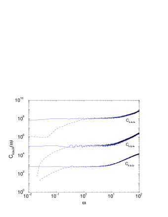
Figure 14: Dependence of the different flux-correlation functions on $\omega$. The solid lines correspond to $\tilde{\mathrm{C}}_{k{\mathrm{J}}_{a}{\mathrm{J}}_{b}}(\omega)$ for $k=1$. The dashed lines are for $k=10$. The dependence on omega of $\tilde{\mathrm{C}}_{k{\mathrm{J}}_{u}{\mathrm{J}}_{\rho}}(\omega)$ is the same that for $\tilde{\mathrm{C}}_{k{\mathrm{J}}_{\rho}{\mathrm{J}}_{u}}(\omega)$ within the numerical accuracy and therefore, not shown.

The periodic microcanonical simulation was performed at an energy corresponding to a temperature $T=150$ with $N=658$ particles. The particles and discs were set up in an equilibrium state, and we allowed the system to further equilibrate by itself before we started the measurements. The energy and particle flux correlation functions were obtained as follows: We measured at each of the $n=1\ldots L$ cells the energy ${\mathrm{J}}_{nu}(t)$ and particle ${\mathrm{J}}_{n\rho}(t)$ currents as a function of time. They were measured at discrete values of time with $\Delta t=0.005$ (which corresponds to approximately a third of the typical time required to traverse the shortest collision path in the system). From these, we obtained the $k$ Fourier component of the fluxes as

$${\mathrm{J}}_{k\rho}(t) = \sum_{n=1}^{L}e^{i2\pi kn/L}{\mathrm{J}}_{n\rho}(t)$$ (31a)

$${\mathrm{J}}_{ku}(t) = \sum_{n=1}^{L}e^{i2\pi kn/L}{\mathrm{J}}_{nu}(t)\ .$$ (31b)

From a time series of $4\times 10^{7}$ data, approximately equivalent to $10^{6}$ times the mean free flight time, we obtained the time averaged Fourier component of the energy and particle flux time-correlation functions

$${\mathrm{C}}_{k{\mathrm{J}}_{a}{\mathrm{J}}_{b}}(t)=\left<{\mathrm{J}}_{ka}(t){\mathrm{J}}_{kb}^{*}(0)\right>_{t}\ .$$ (32)

Finally, we performed the time Fourier transform of these quantities. In Fig. 14 we show the plots of the correlation functions ${\mathrm{C}}_{k{\mathrm{J}}_{a}{\mathrm{J}}_{b}}(w)$, as functions of $\omega$ for values of $k=1$ and $10$. These plots show that at low frequencies the correlations functions tend to zero, in agreement with (27). However, there is a clear plateau in the plots corresponding to the regime in which the Green-Kubo relations hold. At higher frequencies, the curves again deviate from the plateau. This is due to the fact that these high frequencies correspond to times that are shorter than typical collision times, for which the diffusive transport assumptions used to derive (27) no longer hold. Taking the plateau values for the correlation functions, which are essentially independent of $k$ and $\omega$, we can compute the Green-Kubo predictions for the Onsager coefficients using (30). In Table 1, we summarize the values obtained for the different Onsager coefficients and compare them with those obtained previously at this temperature and density.

	Green-Kubo	Gradients
$L_{\rho\rho}$	$0.1050\pm 0.003$	$0.1030\pm 0.002$
$L_{\rho u}$	$0.1276\pm 0.0016$	$0.1271\pm 0.0017$
$L_{u\rho}$	$0.1276\pm 0.0016$	$0.1272\pm 0.0048$
$L_{uu}$	$0.7920\pm 0.012$	$0.7710\pm 0.005$

Table 1: Onsager coefficients calculated from the Green-Kubo formulas (30) compared with those values obtained previously from direct measurements.

An interesting issue involving the linear-response of the system is the macroscopic equivalence between transport processes driven by thermodynamical forces (due to gradients in thermodynamical quantities) and those driven by real forces (like externally applied fields).

It has been argued by van Kampen vanKampen71 that the linear response theory derivation of Green-Kubo formula for the electrical conductivity is not correct as the response of the microscopic trajectories to an applied electric field can not be taken as linear (see also visscher74 ; dorfman99 ). It has been argued by Visscher visscher74 , however, that a difference may exist between the case of mechanical forces, for which van Kampen’s objection might hold, and thermodynamical forces such as temperature and chemical potential gradients, for which linear response should provide correct answers. In order to test this point, we performed simulations for our system in an electric field (all particles having the same charge and no interaction) and compared this with the result of the corresponding gradient in chemical potential.

At the level of the Green-Kubo relations the equivalence follows directly from the linear response results for a chemical potential gradient or an applied electric field: Both are related to the autocorrelation function of the particle current when all particles have the same charge, which is the case in our system.

In order to test these ideas we have performed two complementary simulations: In a first simulation we impose a chemical potential gradient at constant temperature. In a second simulation both temperature and chemical potential are constant and an external uniform electric field is applied to the system in which the particles now carry a unit electric charge $q$. To compare the macroscopic flows obtained in these simulations, the magnitude of the electric field $E$ is fixed to

$$\Delta\mu=qEL\ ,$$ (33)

so that, the work done by the electric field in taking a particle from one side of the channel to the other is the same as the chemical potential difference. In (33), $L$ is the size of the system.

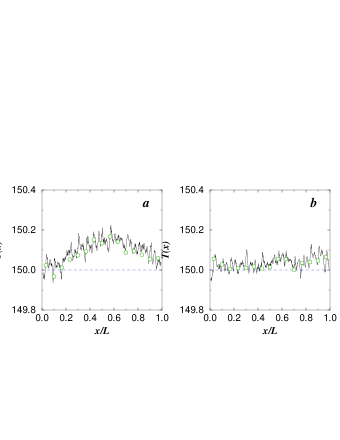
Figure 15: Temperature profiles obtained from a simulation at constant $T=150$ and mean number of particles $N\sim 41.2$ in a channel of length $L=30$ obtained a) from a simulation with constant $\mu$ and a applied electric field of magnitude $E=0.5$. and b) without electric field and an imposed chemical potential gradient of $\nabla(\mu/T)=0.1$. The circles correspond to the averaged kinetic energy of the discs for the respective simulation. The dashed line is the expected value for the profile.

In Fig. 15, the temperature profile of both simulations is compared. When the electric field is applied (Fig. 15-a), the temperature in the bulk of the system increases due to the internal dissipation of the work done by the field. This is the well known Joule heating effect mazur84 . In this case, we have checked that the dependence of the increment of temperature in the bulk $\Delta T$ is quadratic in the field and observed that it holds even far beyond the linear regime. In the case of an imposed chemical potential gradient (Fig. 15-b), the temperature profile appears to be flat, indicating that in this case no effect equivalent to Joule heating is present.

We have also measured the particle density profile and obtained the profile for the quantity $\mu/T$ computed using the relation (6) in both cases. These are shown in Fig. 16-a for the case of an applied electric field and in Fig. 16-b for an imposed chemical potential gradient. In case (a) the chemical potential is flat since we are not taking into account the electric contribution. In case (b) the profile is linear and shows quadratic deviations from linearity similar to those observed for the temperature profile in case (a). This is shown in the inset of Fig. 16-b where we subtracted the theoretical linear $\mu/T$ profile.

Finally, for the heat and matter flows we have obtained for the case of an applied electric field

$$\begin{array}[]{rcl}{\mathrm{J}}_{\rho}&=&-0.00829\pm 0.00006\\ {\mathrm{J}}_{u}&=&-1.59\pm 0.02\ ,\end{array}$$ (34)

and for the case of an imposed chemical potential gradient

$$\begin{array}[]{rcl}{\mathrm{J}}_{\rho}&=&-0.00829\pm 0.00008\\ {\mathrm{J}}_{u}&=&-1.59\pm 0.04\ .\end{array}$$ (35)

Thus, the fluxes obtained in both simulations corroborate our initial expectations within the numerical accuracy.

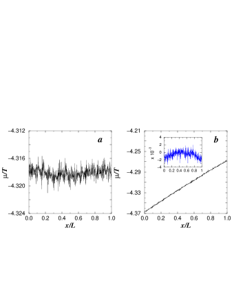
Figure 16: Profiles for the quantity $\mu/T$ minus the expected profile $\mu_{0}/T$ obtained from the simulations described in Fig. 15 with (a) an applied electric field and (b) with an imposed chemical potential gradient.

VII Rates of Entropy Production and Phase Space Volume Contraction

It is generally argued that stationary states are characterized by minimal rate of entropy production. In general, this rate has been at the focus of considerable interest. In particular, in recent work on thermostated systems, the average rate of phase space volume contraction has been identified with the rate of entropy production chernov93 ; holian87 ; moran87 ; chernov93-2 ; ruelle96 ; dorfman99 . While this work is certainly of considerable interest, it is vital to be able to understand how such claims might generalize to purely Hamiltonian systems, for which phase space volume is rigorously conserved, at least in the fine-grained sense, due to Liouville’s theorem. Our system is well-suited to this purpose, since its dynamics is quite transparent and its equilibrium behaviour is trivial.

In our system, it is clear that phase space volume can only be created or annihilated at the boundaries, due to the conservation of phase space throughout the internal dynamics (note that the collision rules (II) are volume preserving). To estimate the variations in phase space volume induced by the incoming and outgoing particles, we proceed as follows: let us denote by $T_{1}$ and $T_{2}$ the two temperatures and by $\mu_{1}$ and $\mu_{2}$ the two chemical potentials at either end of the system (once again, due to LTE there is a local “temperature” and “chemical potential” in the stationary state of the system). A particle entering at one end of the system therefore contributes to the change in phase space volume $\Omega$ by changing both the the local energy per unit volume and the local particle density. Since, as follows from the assumption of LTE, the local thermodynamical variables are connected to each other in the usual way, the increase in phase space volume is given by

$$\Delta\ln\Omega=\sum\limits_{i=1}^{2}\left(\frac{1}{T_{i}}\left(\Delta U\right)_{i}-\frac{\mu_{i}}{T_{i}}\left(\Delta N\right)_{i}\right),$$ (36)

where $i$ can take the values $1$ and $2$ for either end. Due to stationarity, however, it is clear that

$$\begin{array}[]{lclcl}\left(\Delta N\right)_{1}&=&-\left(\Delta N\right)_{2}&=&{\mathrm{j}}_{\rho}\Delta t\\ \left(\Delta U\right)_{1}&=&-\left(\Delta U\right)_{2}&=&{\mathrm{j}}_{u}\Delta t\ .\end{array}$$ (37)

Putting (37) into (36), one obtains the expression for the rate of production of the phase space volume:

$$\frac{d\ln\Omega}{dt}=L\left[-{\mathrm{j}}_{u}\nabla\frac{1}{T}+{\mathrm{j}}_{\rho}\nabla\frac{\mu}{T}\right].$$ (38)

Using (12), and the positive definiteness of the matrix of transport coefficients $L_{\alpha\beta}$, one finds that the r.h.s of (38) is always negative: on the whole, phase space volume flows out of the system into the baths. This can be interpreted in two complementary ways. At first, one might argue that if a system has ever contracting phase space volume, it must eventually end up on an invariant set of measure zero. This is in fact quite reasonable and in good agreement with various findings on the dynamics of reversible thermostated systems. Indeed, various people dorfman99 ; gallavotti95 ; ruelle99 ; evans00 have found that the invariant measure for such systems is singular with respect to Liouville measure. If we were to generalize such an assumption to our system, it would mean that the invariant measure of the stationary state it eventually reaches is also singular with respect to Liouville measure, which would in turn signify that the total phase space volume of the steady state is zero. In principle, this seems amenable to a numerical test, but this is not really the case: due to the rather high dimensionality of our system, the fractality of the support of the steady state measure is presumably extremely difficult to observe, if it is at all possible. Therefore, even if we could connect entropy production, say, with some kind of escape rate (as proposed by Gaspard and coworkers gaspard98 ), it is not at all clear how to measure such a quantity in even so simple a model as ours. Whether truly low-dimensional systems exist, for which such quantities are readily accessible and which also exhibit LTE and normal transport, is an interesting open problem.

Another interpretation of (38) is the following: in the stationary state, because we are in fact in LTE, that is, approximately in a state of thermal equilibrium in every volume element, we may think that at least the coarse grained phase space volume, measured by the thermodynamical entropy, will remain constant in steady state. But if, as claimed in (38), an amount of phase space volume leaves the system each unit of time, then an equivalent amount of coarse-grained phase space volume must be produced inside the system. That this last statement does not contradict Liouville’s theorem is, of course, well-known from traditional examples in statistical mechanics. Such an interpretation might then justify the interpretation of the r.h.s of (38) as minus the rate of entropy production, in conformity with the results stated for reversible thermostated systems.

To make such an identification plausible, we need a definition of the entropy out of equilibrium. It is well-known that in the general case such a definition poses formidable problems. However, since our system is an ideal gas but little perturbed from equilibrium, it is possible to use Boltzmann’s expression for an entropy density per unit volume in terms of the one-particle distribution function $f(x,v;t)$, defined by

$$s(x)=-\int dv\,f(x,v;t)\ln f(x,v;t)$$ (39)

From this one may give an elementary expression for the rate of entropy production through the following considerations. Due to LTE, the stationary distribution $f(x,v)$ is given by a local Maxwellian

$$f(x,v)=\rho(x)\beta(x)^{1/2}\exp\left[-\beta(x)v^{2}/2\right]+\delta f(x,v)$$ (40)

where $\delta f(x,v)$ is a correction term of the order of the imposed gradients, which accounts for the currents in the system. As shown in (9) such a correction has been observed in our system. It then seems reasonable to divide the time variation of $f(x,v)$ into a convective part given by $-vf_{x}$ plus a collisional part, of which we need say nothing. In this case, we may define the entropy current density as follows

$${\mathrm{j}}_{s} = -\int dv\,vf(x,v)\ln f(x,v)$$ (41)

$$= -\int dv\,v\delta f(x,v)[\ln f(x,v)+1]\ .$$ (42)

Inserting (40) into (LABEL:eq:current) yields

$${\mathrm{j}}_{s}=-\frac{\mu}{T}{\mathrm{j}}_{\rho}+\frac{1}{T}{\mathrm{j}}_{u}\ .$$ (44)

In the stationary state, the local rate of entropy production is given by the divergence of the entropy current. If one takes it as given by (44), we obtain again the rate of entropy production given by the standard expression, this time with the correct positive sign.

VIII Conclusion

We have introduced a simple model system characterized by reversible Hamiltonian microscopic dynamics, the equilibrium properties of which are those of an ideal gas when viewed as a thermodynamic system. We performed extensive numerical studies of the system both in equilibrium and in non-equilibrium steady state. We find that when driven out of equilibrium, the properties of the system are consistent with the hypothesis of local thermal equilibrium, that is, in the stationary state, one finds a local Boltzmann distribution for the energies, leading therefore to an unambiguous definition of the local temperature, chemical potential, etc. In this situation its transport properties are found to be entirely similar to those of realistic interacting many particle systems: it exhibits coupled mass and heat transport and the two cross transport coefficients satisfy Onsager’s relations. When time reversal invariance is broken by means of an applied constant magnetic field, the appropriate generalizations of the Onsager relations hold. This is the case even though this system turns out not to be ergodic. Furthermore, we find extremely satisfactory agreement between the values of the transport coefficients as deduced from the equilibrium dynamics via the Green–Kubo formulas and those obtained via direct simulation. A final result of interest is that we were able to show equivalence between an applied electric field and a chemical potential gradient. This result, while a straightforward consequence of linear response, does not appear at all obvious from the microscopic point of view. It may therefore be considered as a further confirmation of the validity of the linear response formalism

The fact that all these features are present in such a simple model, suggests that it may serve as an ideal framework to gain insight of how macroscopic transport phenomena arise in real systems. The model is also well suited to test theories for the description of systems in out of equilibrium states. Among these, a study of the Cohen–Gallavotti theorem might be very interesting. Also, issues linked to those involving entropy production discussed in the section VII, in particular the question of characterizing the invariant measure of the stationary state appears very challenging.

Finally, extensions to more complicated systems can also be considered. By varying the value of the moment of inertia of the rotors one can study transport in heterogeneous structures, such as junctions, layered systems, etc. Other extensions could include mixtures of scattered particles with different masses. For all these extensions, most if not all of the equilibrium properties are straight forward, and theories for the phenomenological behaviour of such systems can be carefully tested.

Appendix A Various Possible Thermo-chemical Baths

In this appendix we present a short discussion of Markov processes that can be used to generate a canonical or grand canonical ensemble. A fairly general Markov process combined with a Hamiltonian dynamics satisfies the master equation

$$\partial_{t}\rho_{N}(x) = \{H_{N},\rho_{N}\}+\sum_{N^{\prime}}\int W(N^{\prime}N;x^{\prime}x)\rho_{N^{\prime}}(x^{\prime})dx^{\prime}-$$ (45)

$$-\rho_{N}(x)\sum_{N\neq N^{\prime}}\int W(NN^{\prime};xx^{\prime})dx^{\prime}.$$

Here $N$ is the number of particles, $x$ is an abbreviated notation for the vector $(p,q)$ and $\rho_{N}(x)$ is the probability density of being at the phase point $x$ having altogether $N$ particles. The $W(NN^{\prime};xx^{\prime})$ are the transition rates of going from a phase point $x$ with $N$ particles to a phase point $x^{\prime}$ with $N^{\prime}$ particles. If we are looking for rates such that they generate, say, the grand canonical ensemble with a given temperature and chemical potential, it is sufficient that they satisfy the detailed balance condition

$$\frac{W(NN^{\prime};xx^{\prime})}{W(N^{\prime}N;x^{\prime}x)}=\exp[\beta\mu(N-N^{\prime})-\beta(H_{N^{\prime}}(x^{\prime})-H_{N}(x))].$$ (46)

Let us now assume that the stochastic part of the dynamics is limited to the case in which $x$ belongs to a small subset $\Gamma$ of the full phase space, otherwise the dynamics is purely Hamiltonian. This corresponds to the case of stochastic walls treated in this paper. Assume further that, as in our model, the Hamiltonian in $\Gamma$ is one-particle only, say a pure kinetic energy term. Assume finally that the only changes we consider will be the introduction and destruction of a single particle. Then the following rates are a solution of (46):

$$W_{\Gamma}(N,N+1)=\lambda e^{-\beta(\frac{v^{2}}{2}+\mu)}\qquad W_{\Gamma}(N+1,N)=\lambda$$ (47)

If we want this stochastic process to act as a localized bath in the system, we take the region $\Gamma$ in phase space defined by the condition that at least one particle is in the region $V$ of the (one-particle) configuration space. The rates in (47) then mean that any particle entering $V$ is annihilated at a rate $\lambda$. Further, particles of speed $v$ are being created inside $V$ at a rate $\lambda e^{-\beta(\frac{v^{2}}{2}+\mu)}$. Since such particles may be immediately reabsorbed, however, the problem of the particle flux emitted by $V$ is not quite straightforward. If $V$ is narrow (of thickness $l$) in one dimension around a given hypersurface $S$, however, and $\lambda$ is ultimately made to go to infinity as $l\to 0$, the problem can be solved as follows. For simplicity, assume that all momenta always point in the direcion of one of the sides of $V$. The probability that the particle will come out at all, conditioned on its having been created at a distance $r$ of the side from which it must leave $V$ is given by

$$p(r)=\exp\left[-\lambda r/v_{n}\right],$$ (48)

where $v_{n}$ is the velocity normal to the surface $S$. The flux of particles coming out of $V$ is then given by

$$\lambda e^{-\beta v^{2}/2}\int_{0}^{l}dr\,p(r)=v_{n}e^{-\beta v^{2}/2+\beta\mu}\left(1-e^{-\alpha/v_{n}}\right),$$ (49)

where $\alpha$ is the limiting value of $\lambda l$. In the limit in which $\alpha\to\infty$, this model reduces to the one described in the text, which was the one primarily used in the simulations presented in this paper. The above model can be generalized in different ways: in particular, we may allow for thermalization without change in the number of particles. A possible candidate for such a reaction rate is given by

$$W(NN;xx^{\prime})=\lambda^{\prime}\exp\left[-\beta(v^{\prime}{}^{2}-v^{2})/2\right]\delta(q-q^{\prime}),$$ (50)

where again the process acts only in the region $\Gamma$ described above. This corresponds to a process in which the particle velocities are thermalized while leaving their positions fixed, which is, as is readily seen, the algorithm for thermalization through collisions introduced in the text. In particular, the case $\alpha=0$ and a finite rate of the type given is (50) leads to the algorithm we used for generating the canonical ensemble.

Various simulations were made with finite values of $\alpha$ in order to test the method. In equilibrium it was always found that the correct nominal temperatures and chemical potentials were attained after sufficient time. In non-equilibrium situations, however, for small values of $\alpha$, the thermodynamic parameters of the system can differ from the values imposed by the baths. In particular, the energy density showed jumps localized in the vicinity of the walls. These energy gaps have been frequently observed in simulations of other transport models prosen92 ; lepri97 ; lepri98 ; hatano99 ; aoki00 and were studied in aoki01 . In our model, they eventually disappear as we increase the value of $\alpha$, meaning that the absorption of the wall increases and the particles (which thermalize the system with the bath) are exchanged more easily.

References

- (1) F. Bonetto, J.L. Lebowitz and L. Rey-Bellet, arXiv:math-ph/0002052, (2001)
- (2) J.L. Lebowitz and H. Spohn, J. Stat. Phys. 19, 633 (1978)
- (3) J.L. Lebowitz and H. Spohn, J. Stat. Phys. 28, 539 (1982)
- (4) L.A. Bunimovich and Ya.G. Sinai, Comm. Math. Phys. 78, 247 (1980); L.A. Bunimovich and Ya.G. Sinai, Comm. Math. Phys. 78, 479 (1981); P. Gaspard, J. Stat. Phys. 68, 673 (1992); J.R. Dorfman and P. Gaspard, Phys. Rev. E 51, 28 (1995)
- (5) N.I. Chernov, G.L. Eyink, J.L. Lebowitz and Ya.G. Sinai, Comm. Math. Phys. 154, 569 (1993)
- (6) B. L. Holian, W. G. Hoover, and H. A. Posch, Phys. Rev. Lett. 59, 10 (1987)
- (7) B. Moran, W. G. Hoover , J. Stat. Phys. 48, 709 (1987)
- (8) . I. Chernov, G. L. Eyink, J. L. Lebowitz, and Y. G. Sinai, Phys. Rev. Lett. 70, 2209 (1993)
- (9) D. MacGowan and D.J. Evans, Phys. Rev. A 34, 2133 (1986)
- (10) S. Lepri, R. Livi and A. Politi, Phys. Rev. Lett. 78, 1896 (1997)
- (11) G. Casati, J. Ford, F. Vivaldi and W.M. Visscher, Phys. Rev. Lett. 52, 1861 (1984)
- (12) T. Prosen and M. Robnik, J. Phys. A:Math. Gen. 25, (1992) 3449
- (13) L. Rondoni and E.G.D. Cohen, Physica D 168-169, 341 (2002)
- (14) E.G.D. Cohen and L. Rondoni, Physica A 306, 117 (2002)
- (15) D. Alonso, R. Artuso, G. Casati and I. Guarneri, Phys. Rev. Lett. 82, 1859 (1999)
- (16) A. Dhar and D. Dhar, Phys. Rev. Lett. 82, 480 (1999)
- (17) B. Hu, B. Li and H. Zhao, Phys. Rev. Lett. 82, 480 (1998)
- (18) T. Prosen and D. K. Campbell, Phys Rev. Lett. 84, 2857 (2000)
- (19) C. Mejia-Monasterio, H. Larralde and F. Leyvraz, Phys. Rev. Lett. 86, 5417, (2001)
- (20) L. Reichl, A Modern Course in Statistical Physics (Austin University of Texas Press, 1987)
- (21) K. Rateitschack, R. Klages and G. Nicolis, J. Stat. Phys. 99, 1339, (2000)
- (22) Due to the homogeneity in energy of this system there is not no proper energy scale or equivalently, no proper time scale. Therefore, all energies and temperatures reported in this work are given in arbitrary units.
- (23) R. Tehver, F. Toigo, J. Koplik and J.R. Banavar, Phys. Rev. E. 57, R17 (1998)
- (24) T. Hatano, Phys. Rev. E, 59, R1 (1999)
- (25) Actually, the obtained average velocity was , which is of the same order of the particle current . We have also measured the deviations from the Maxwell distribution for huge gradients in the chemical potential, far from the linear regime. There, while the deviations are much clearer, not just in the average velocity but in the width of the distribution too, their relative value is still of .
- (26) S. R. de Groot and P. Mazur, Non-equilibrium Thermodynamics (Dover, New York, 1984).
- (27) We derive Green-Kubo relations for the diffusion coefficients that involve the collective heat and matter transport we observe. The self-diffusion coefficient, obtained from the velocity auto-correlation function of a tagged particle diffusing in a fluid of identical particles coincides with the diffusion coefficient only for systems with noninteracting particles. See also, Y.Zhaou and G. H. Miller, J. Phys. Chem. 100, 5516 (1996)
- (28) N. G. van Kampen, Phys. Norv. 5, 279 (1971)
- (29) W. M. Visscher, Phys. Rev. A, 10, 2461 (1974)
- (30) D. Ruelle, J. Stat. Phys. 85,1 (1996)
- (31) J. R. Dorfman, An introduction to Cahos in Nonequilibrium Statistical Mechanics (Cambridge University Press, Cambridge 1999)
- (32) G. Gallavotti and E. G. D. Cohen, J. Stat. Phys. 80, 931 (1995); Phys. Rev. Lett. 74, 2694 (1995)
- (33) D. Ruelle, J. Stat. Phys. 95, 393 (1999)
- (34) D. J. Evans, E. G. D. Cohen, D. Searles and F. Bonetto, J. Stat. Phys 101, 17 (2000)
- (35) P. Gaspard, Chaos, Scattering and Statistical Mechanics (Cambridge University Press, Cambridge 1998)
- (36) S. Lepri, R. Livi and A. Politi, Physica D, 119, 140 (1998)
- (37) K. Aoki and D. Kusnezov, Phys. Lett. A, 265, 250 (2000)
- (38) A. Dhar, Phys. Rev. Lett. 86, 3554 (2001)
- (39) K. Aoki and D. Kusnezov, Phys. Rev. Lett. 86, 4029 (2001)